1 Introduction
We consider the two-dimensional nonlinear problem describing steady waves in a horizontal open channel of uniform rectangular cross-section. The motion of an inviscid, incompressible, heavy fluid, say water, occupying the channel is supposed to be rotational with a prescribed vorticity distribution. The reason for considering this mathematical model is the importance of vorticity for interaction of waves with currents (see Peregrine Reference Peregrine1976). This interaction commonly occurs in nature as is indicated by observations – see, for example, Swan, Cummins & James (Reference Swan, Cummins and James2001) and references cited therein. An interesting phenomenon predicted in the framework of this model is the formation of (possibly multiple) counter-currents separated one from the other by critical layers – see Wahlén (Reference Wahlén2009), Ehrnström, Escher & Wahlén (Reference Ehrnström, Escher and Wahlén2011), Ehrnström, Escher & Villari (Reference Ehrnström, Escher and Villari2012) and Kozlov & Kuznetsov (Reference Kozlov and Kuznetsov2014) and references cited therein.
The aim of the present article is to study the whole set of waves on unidirectional flows that correspond to near-critical values of Bernoulli’s constant. It should be noted that waves exist only when the constant is greater than its critical value and the complexity of wave patterns grows as the value increases. However, it occurs that the behaviour of waves with vorticity in the near-critical regime is similar to that in the irrotational case. In particular, the Benjamin–Lighthill conjecture (the topic of this paper) is true.
The original conjecture describes irrotational wave trains in terms of three parameters, namely,
 $Q$
(rate of flow),
 $R$
(total head/Bernoulli’s constant) and
 $S$
(flow force); each of these parameters is a constant of wave motion, that is, it does not depend on the coordinate measured along the horizontal bottom. The hydrodynamic meaning of the first two is clear from their names, whereas the flow force is proportional to the sum of horizontal momentum flux and pressure force. This parameter is essential for representation of problems for irrotational and rotational steady waves in Hamiltonian form – see the papers by Mielke (Reference Mielke1991), Kozlov & Kuznetsov (Reference Kozlov and Kuznetsov2013b
) and Groves & Stylianou (Reference Groves and Stylianou2014). Benjamin (Reference Benjamin1984, § 4.4) had emphasised the role of this parameter as a recipe for studying general steady-wave problems governed by elliptic equations.
Let
 $r$
and
 $s$
denote the non-dimensional versions of
 $R$
and
 $S$
, respectively, corresponding to some
 $Q$
(see § 1.2 for details). Let
 ${\mathcal{C}}$
be the region in the
 $(r,s)$
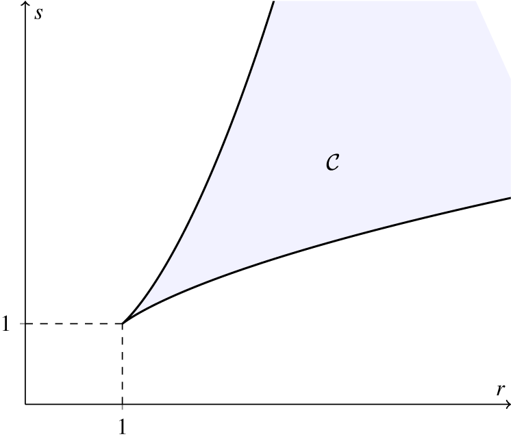
plane (see figure 1, a scaled version of figure 2 in Benjamin & Lighthill (Reference Benjamin and Lighthill1954)), whose cusped boundary
 $\unicode[STIX]{x2202}{\mathcal{C}}$
represents all possible uniform streams; moreover, the part of
 $\unicode[STIX]{x2202}{\mathcal{C}}$
corresponding to supercritical streams (the lower curve) is included into
 ${\mathcal{C}}$
, whereas the other part is not. The Benjamin–Lighthill conjecture says that:
-
(1) each wave train is represented by a point of
 ${\mathcal{C}}$
;
-
(2) every point of
${\mathcal{C}}$
corresponds to some wave train.


In 2010–11, this form of the conjecture was proved by Kozlov and Kuznetsov for irrotational waves corresponding to near-critical values of Bernoulli’s constant; in other words, for the pairs
 $(r,s)$
belonging to a vicinity of the tip of
 ${\mathcal{C}}$
.
Values of
 $(r,s)$
representing possible steady irrotational waves according to Benjamin & Lighthill (Reference Benjamin and Lighthill1954).

Here, we modify the Benjamin–Lighthill conjecture to adapt it for rotational waves on unidirectional flows. Let
 $\unicode[STIX]{x1D714}$
be a vorticity distribution; then the corresponding region
 ${\mathcal{C}}_{\unicode[STIX]{x1D714}}$
(its boundary represents all possible horizontal shear flows) has its cusp at
 $(r_{c},s_{c})$
and is truncated by the line
 $r=r_{0}$
, where the constants
 $r_{c}$
,
 $s_{c}$
and
 $r_{0}$
are defined by
 $\unicode[STIX]{x1D714}$
(see §§ 2.1 and 2.2), and
 $r_{0}$
can be finite for some vorticity distributions and infinite for others. Under the assumptions that
 $\unicode[STIX]{x1D714}$
is Lipschitz continuous and the problem’s parameter
 $r$
attains near-critical values (that is,
 $r-r_{c}$
is small, and so
 $s-s_{c}$
is also small because
 $s$
is a function of
 $r$
), we prove the following extended version of the conjecture. Namely, along with the assertions (1) and (2) formulated above we show that the correspondence between wave trains and points in
 ${\mathcal{C}}_{\unicode[STIX]{x1D714}}$
is one-to-one.
To verify the conjecture we establish that amplitudes and slopes are arbitrarily small for waves on near-critical rotational flows and the smallness depends on how close
 $r$
is to
 $r_{c}$
. This was also done in the irrotational case, but here we use a new method for this purpose and it differs essentially from that in Kozlov & Kuznetsov (Reference Kozlov and Kuznetsov2010, Reference Kozlov and Kuznetsov2011a
), where harmonic analysis was applied for waves without vorticity. Our approach provides explicit descriptions of the whole family of waves existing for every near-critical value of Bernoulli’s constant. Namely, there are two different parametrisations for the family of waves having their crests on a fixed vertical line.
1.1 Statement of the problem
Let an open channel of uniform rectangular cross-section be bounded below by a horizontal rigid bottom and let water occupying the channel be bounded above by a free surface not touching the bottom. In appropriate Cartesian coordinates
 $(x,y)$
, the bottom coincides with the
 $x$
-axis and gravity acts in the negative
 $y$
-direction. We use the non-dimensional variables proposed by Keady & Norbury (Reference Keady and Norbury1978) (see also appendix A in Kozlov & Kuznetsov (Reference Kozlov and Kuznetsov2014) for details of scaling), namely, the constant volume rate of flow per unit span and the constant acceleration due to gravity are scaled to unity in our equations. For this purpose, lengths and velocities are scaled to
 $(Q^{2}/g)^{1/3}$
and
 $(Qg)^{1/3}$
, respectively. Here
 $Q$
and
 $g$
are the dimensional quantities for the rate of flow and the gravity acceleration, respectively, whereas
 $(Q^{2}/g)^{1/3}$
is the depth of the critical uniform stream in the irrotational case (see e.g. Benjamin Reference Benjamin1995).
The steady water motion is assumed to be two-dimensional and rotational; the surface tension is neglected on the free surface, where the pressure is constant. These assumptions and the fact that water is incompressible allow us to seek the velocity field in the form
 $(\unicode[STIX]{x1D713}_{y},-\unicode[STIX]{x1D713}_{x})$
, where
 $\unicode[STIX]{x1D713}(x,y)$
is referred to as the streamfunction. The vorticity distribution
 $\unicode[STIX]{x1D714}$
is assumed to be a prescribed Lipschitz function depending on
 $\unicode[STIX]{x1D713}$
.
We choose the frame of reference so that the velocity field is time-independent as well as the unknown free-surface profile. The latter is assumed to be the graph of
 $y=\unicode[STIX]{x1D702}(x)$
,
 $x\in \mathbb{R}$
, where
 $\unicode[STIX]{x1D702}$
is a positive continuous function, and so the longitudinal section of the water domain is
 $D=\{x\in \mathbb{R},~0<y<\unicode[STIX]{x1D702}(x)\}$
. The following free-boundary problem for
 $\unicode[STIX]{x1D713}$
and
 $\unicode[STIX]{x1D702}$
which describes all kinds of waves has long been known (cf. Keady & Norbury Reference Keady and Norbury1978):
 $$\begin{eqnarray}\displaystyle & \displaystyle \unicode[STIX]{x1D713}_{xx}+\unicode[STIX]{x1D713}_{yy}+\unicode[STIX]{x1D714}(\unicode[STIX]{x1D713})=0,\quad (x,y)\in D, & \displaystyle\end{eqnarray}$$
 $$\begin{eqnarray}\displaystyle & \displaystyle \unicode[STIX]{x1D713}(x,0)=0,\quad x\in \mathbb{R}, & \displaystyle\end{eqnarray}$$
 $$\begin{eqnarray}\displaystyle & \displaystyle \unicode[STIX]{x1D713}(x,\unicode[STIX]{x1D702}(x))=1,\quad x\in \mathbb{R}, & \displaystyle\end{eqnarray}$$
 $$\begin{eqnarray}\displaystyle & \displaystyle |\unicode[STIX]{x1D735}\unicode[STIX]{x1D713}(x,\unicode[STIX]{x1D702}(x))|^{2}+2\unicode[STIX]{x1D702}(x)=3r,\quad x\in \mathbb{R}. & \displaystyle\end{eqnarray}$$
In condition (1.4) (Bernoulli’s equation),
 $r$
is a constant referred to as the total head (Bernoulli’s constant); it is considered as the problem’s parameter.
Initially, it is natural to impose rather weak assumptions on the unknown functions, namely, that
 $\unicode[STIX]{x1D713}\in C_{loc}^{1}(\bar{D})$
and
 $\unicode[STIX]{x1D702}$
is a Lipschitz function on
 $\mathbb{R}$
. This allows us to understand the boundary value problem (1.1)–(1.3) in a weak sense. Then the classical Schauder estimates are applicable because
 $\unicode[STIX]{x1D714}$
is a Lipschitz function. This implies that
 $\unicode[STIX]{x1D713}\in C^{2,\unicode[STIX]{x1D6FC}}(D)$
for every
 $\unicode[STIX]{x1D6FC}\in (0,1)$
, and so problem (1.1)–(1.4) may be understood in the classical sense. Indeed,
 $\unicode[STIX]{x1D735}\unicode[STIX]{x1D713}$
is continuous up to the boundary, which yields that (1.4) is fulfilled in the classical sense.
We are going to study only unidirectional flows (this is natural when
 $r$
is near-critical; see figure 3), in which case the horizontal component of the velocity field has the same direction, say to the right, throughout the flow. This assumption results in the following additional condition:
 $$\begin{eqnarray}\unicode[STIX]{x1D713}_{y}(x,y)>0\quad \text{for all}~(x,y)\in \bar{D}.\end{eqnarray}$$
In conclusion of this section, we recall that
 $(\unicode[STIX]{x1D713},\unicode[STIX]{x1D702})$
is called a Stokes-wave solution of problem (1.1)–(1.5) when
 $\unicode[STIX]{x1D702}$
is a periodic function with a single crest per wavelength and symmetric about vertical lines going through crests, whereas
 $\unicode[STIX]{x1D713}(x,y)$
is a periodic function of
 $x$
and its period is the same as that of
 $\unicode[STIX]{x1D702}$
. Furthermore, a non-stream solution
 $(\unicode[STIX]{x1D713},\unicode[STIX]{x1D702})$
is called a solitary-wave solution if it asymptotes some stream solution as
 $|x|\rightarrow \infty$
and
 $\unicode[STIX]{x1D702}$
is symmetric about the vertical line going through the single crest. The class of stream solutions is analogous to uniform irrotational streams and is described below in § 2.1.
1.2 Background
To compare the results obtained for rotational and irrotational waves, we recall what is known in both cases about the whole class of steady waves. The first paper concerning this class in the irrotational case was Benjamin & Lighthill (Reference Benjamin and Lighthill1954), in which it was conjectured that the parameters
 $Q$
,
 $R$
and
 $S$
‘probably determine the wave-train uniquely’.
In order to formulate the irrotational Benjamin–Lighthill conjecture in precise terms, we recall that both periodic and solitary waves bifurcate from uniform streams whose depths are defined by the following equation:
 $$\begin{eqnarray}\left(\frac{Q}{{\mathcal{H}}}\right)^{2}+2g{\mathcal{H}}=2R,\quad {\mathcal{H}}>0,\end{eqnarray}$$
where
 $Q$
and
 $R$
are given and
 $g$
is the acceleration due to gravity. Namely, let
 $Q$
be fixed, then for
 $R=R_{c}=(3/2)(Qg)^{2/3}$
there exists only one positive root of (1.6) – the double root
 ${\mathcal{H}}_{c}=(Q^{2}/g)^{1/3}$
. The corresponding uniform stream is called critical because for
 $R<R_{c}$
there are no positive roots at all, whereas for
 $R>R_{c}$
the equation has two positive roots
 ${\mathcal{H}}_{-}$
and
 ${\mathcal{H}}_{+}$
such that
 ${\mathcal{H}}_{-}<{\mathcal{H}}_{c}<{\mathcal{H}}_{+}$
. The uniform stream whose depth is equal to
 ${\mathcal{H}}_{-}$
(
 ${\mathcal{H}}_{+}$
) is called supercritical (subcritical, respectively).
We recall that the flow force is proportional to the sum of horizontal momentum flux and pressure force, namely,
 $$\begin{eqnarray}S(X)=\frac{2}{3}\int _{0}^{\unicode[STIX]{x1D709}(X)}[V_{(X)}^{2}(X,Y)+p(X,Y)]\,\text{d}Y.\end{eqnarray}$$
Here
 $(X,Y)$
and
 $\unicode[STIX]{x1D709}(X)$
are dimensional coordinates and the free surface profile, respectively,
 $V_{(X)}$
is the horizontal component of the velocity vector and
 $p(X,Y)$
is the pressure.
Using
 $R_{c}$
and
 $S_{c}=(3/2)(Q^{4}g)^{1/3}$
(the critical values of
 $R$
and
 $S$
, respectively), two non-dimensional characteristics of flows supporting waves are defined as follows:
 $$\begin{eqnarray}r=R/R_{c},\quad s=S/S_{c},\end{eqnarray}$$
of which
 $r$
is usually considered as a given parameter in the problem yielding streamfunction and wave profile. Meanwhile, the expression for
 $s$
derived from (1.7) depends on the problem’s solution as well as on
 $r$
itself, namely, we have
 $$\begin{eqnarray}s=s(\unicode[STIX]{x1D713},\unicode[STIX]{x1D702})=r\unicode[STIX]{x1D702}(x)-\frac{1}{3}\unicode[STIX]{x1D702}^{2}(x)+\frac{1}{3}\int _{0}^{\unicode[STIX]{x1D702}(x)}[\unicode[STIX]{x1D713}_{y}^{2}-\unicode[STIX]{x1D713}_{x}^{2}]\,\text{d}y,\end{eqnarray}$$
and this formula coincides with (2.4) in Benjamin (Reference Benjamin1995). If
 $r>1$
, then according to this formula we have the following. The value of
 $s$
corresponding to a supercritical stream is equal to
 $s_{-}(r)=(2+\unicode[STIX]{x1D708}_{-})/(3\unicode[STIX]{x1D708}_{-}^{1/3})$
, whereas
 $$\begin{eqnarray}s_{+}(r)=\frac{1}{3\unicode[STIX]{x1D708}_{+}^{1/3}}\left[2+\unicode[STIX]{x1D708}_{+}+\frac{1}{8}\left(\frac{{\mathcal{H}}_{+}}{{\mathcal{H}}_{-}}-1\right)(3-\sqrt{1+8\unicode[STIX]{x1D708}_{+}})^{2}\right]\end{eqnarray}$$
corresponds to a subcritical one. Here,
 $\unicode[STIX]{x1D708}_{-}>1$
 $(\unicode[STIX]{x1D708}_{+}<1)$
is the larger (smaller, respectively) positive root of the following equation:
 $$\begin{eqnarray}r=\frac{1+2\unicode[STIX]{x1D708}}{3\unicode[STIX]{x1D708}^{2/3}}.\end{eqnarray}$$
It is worth mentioning that
 $\unicode[STIX]{x1D708}_{-}$
 $(\unicode[STIX]{x1D708}_{+})$
is the Froude number squared of the supercritical (subcritical, respectively) uniform stream. Both
 $s_{-}(r)$
and
 $s_{+}(r)$
increase monotonically with
 $r$
, and
 $s_{+}(r)>s_{-}(r)$
for all
 $r>1$
, thus defining the cuspidal region
 $$\begin{eqnarray}{\mathcal{C}}=\{(r,s):~1\leqslant r,~s_{-}(r)\leqslant s<s_{+}(r)\}\end{eqnarray}$$
(see figure 1). Here, all pairs of the form
 $(r,s_{-}(r))$
corresponding to supercritical uniform streams are included because they also represent solitary-wave disturbances of these streams when they exist. In terms of
 ${\mathcal{C}}$
the Benjamin–Lighthill conjecture is as follows:
-
(1) every steady wave train is represented by a point in
${\mathcal{C}}$
; -
(2) to every point in
${\mathcal{C}}$
there corresponds some steady wave train; -
(3) the correspondence between wave trains and points in
${\mathcal{C}}$
is one-to-one.


Benjamin & Lighthill (Reference Benjamin and Lighthill1954) (see also Benjamin Reference Benjamin1995) demonstrated that this conjecture is true in the framework of a one-dimensional approximate theory derived under the assumption that both
 $r-1$
and
 $s-1$
are small, that is, waves are long and of small amplitude.
Since no steady waves other than Stokes and solitary waves had been known when the conjecture was proposed, first results confirming assertion (1) were obtained for Stokes waves; namely, Keady & Norbury (Reference Keady and Norbury1978) (see also Benjamin Reference Benjamin1995) proved that Stokes waves are represented by inner points of
 ${\mathcal{C}}$
. On the other hand, Ovsyannikov (Reference Ovsyannikov1980) conjectured that each pair
 $(r,s_{-}(r))$
uniquely determines a solitary wave, but Plotnikov (Reference Plotnikov1992) disproved this conjecture. He established that there are values of
 $r$
for which at least two geometrically distinct solitary-wave profiles exist. Thus, assertion (3) of the Benjamin–Lighthill conjecture does not hold in its general form. It is worth mentioning that as early as 1974 Plotnikov’s result had been found numerically by Longuet-Higgins & Fenton (Reference Longuet-Higgins and Fenton1974).
Further results confirming the conjecture are as follows. Amick & Toland (Reference Amick and Toland1981) showed that
 $r>1$
for solitary waves (another proof of this fact was given by McLeod (Reference McLeod1984)). Subsequently, this fact was proved by Kozlov & Kuznetsov (Reference Kozlov and Kuznetsov2009) for all steady waves irrespective of the type (Stokes, solitary, whatever). On the other hand, numerical results obtained by Cokelet (Reference Cokelet1977) show that assertion (2) is not true, at least for Stokes waves. There is a bound dividing
 ${\mathcal{C}}$
so that all Stokes-wave solutions lie to the left of it. This bound is formed by points corresponding to waves that have greatest total head and flow force for a given wavelength; the corresponding line crosses the lower part of
 $\unicode[STIX]{x2202}{\mathcal{C}}$
at some distance from the cusp vertex and approaches the curve (1.10) for large values of
 $r$
(see figure 1(a) in Keady & Norbury Reference Keady and Norbury1978). Further important results were obtained by Amick & Toland (Reference Amick and Toland1981), who combined the existence theorems for Stokes and solitary waves with the proof of the convergence of Stokes waves to solitary ones in the long-wave limit.
In the near-critical case, that is, when
 $r$
is close to one, the general structure of the whole set of irrotational waves was investigated by Kozlov & Kuznetsov (Reference Kozlov and Kuznetsov2010, Reference Kozlov and Kuznetsov2011a
). It is as follows: only solitary and Stokes waves exist and they are parametrised by the depth at the crest, which varies from the depth of the subcritical uniform flow to that of the solitary wave at its crest. This implies that assertions (1) and (2) of the conjecture are true in this case. Moreover, this hierarchy of waves is in agreement with the one-dimensional approximate theory investigated by Benjamin & Lighthill (Reference Benjamin and Lighthill1954) as well as with the bound obtained by Cokelet (Reference Cokelet1977).
Now, we turn to results for waves with an arbitrary distribution of vorticity. To the authors’ knowledge, so far only Groves & Wahlén (Reference Groves and Wahlén2008) have studied small-amplitude Stokes and solitary waves using a unified approach based on the so-called spatial dynamics in which the horizontal coordinate plays the role of time in a Hamiltonian system with one degree of freedom that is locally equivalent to problem (1.1)–(1.5). Their analysis of this system based on a centre-manifold technique demonstrates the existence of a continuous branch of wave solutions that consists of a solitary wave of elevation and a family of Stokes waves.
2 Main results
A phenomenon’s qualitative account, namely, its phase portrait, is given for small-amplitude waves with vorticity in the above-mentioned paper by Groves & Wahlén (Reference Groves and Wahlén2008). However, for a justification of the Benjamin–Lighthill conjecture this description must be complemented by the following quantitative details: (1) the absence of large-amplitude waves must be demonstrated; (2) a parametrisation for the family of waves corresponding to a given near-critical value of
 $r$
must be obtained (it occurs that there are two different parametrisations); and (3) stability estimates guaranteeing the parametrisation’s continuity must be proved. To provide these properties is the goal of this paper; see theorems formulated in § 2.3, whereas the strategy of their proof is outlined in § 2.4.
The exact formulation of the Benjamin–Lighthill conjecture for waves with vorticity includes the same assertions (1)–(3) as in the irrotational case. However, the vorticity distribution must be involved in the definition of the corresponding cuspidal region (hence this region will be denoted by
 ${\mathcal{C}}_{\unicode[STIX]{x1D714}}$
in what follows) along with the total head
 $r$
and the flow force invariant
 $s$
. The latter is introduced below following Keady & Norbury (Reference Keady and Norbury1978). Similarly to the irrotational case, we define
 ${\mathcal{C}}_{\unicode[STIX]{x1D714}}$
in terms of unidirectional horizontal shear flows which are analogous to uniform streams. In addition, stream solutions describing these flows have more complicated structure. For example, there are several definitions of the so-called Froude number for shear flows, none of which is universal like that for the irrotational uniform streams (see Wheeler (Reference Wheeler2015, p. 95), where these definitions are listed). Therefore, prior to the formulation of the main results, we outline basic properties of stream solutions and provide a classification of vorticity distributions based on these properties. This classification is also important when defining the cuspidal region
 ${\mathcal{C}}_{\unicode[STIX]{x1D714}}$
.
2.1 Stream solutions
By a stream (shear-flow) solution we mean a pair
 $(u(y),d)$
, where
 $u$
stands for the streamfunction instead of
 $\unicode[STIX]{x1D713}$
and the constant depth of flow
 $d$
replaces the wave profile
 $\unicode[STIX]{x1D702}$
. Then problem (1.1)–(1.4) reduces to the following one:
 $$\begin{eqnarray}u^{\prime \prime }+\unicode[STIX]{x1D714}(u)=0~\text{on }(0,d),\quad u(0)=0,\quad u(d)=1,\quad |u^{\prime }(d)|^{2}+2d=3r.\end{eqnarray}$$
Here and below,
 $^{\prime }$
denotes differentiation with respect to
 $y$
. A detailed study of these solutions including those that describe flows with counter-currents is given in Kozlov & Kuznetsov (Reference Kozlov and Kuznetsov2011b
). In particular, it is shown that the set of unidirectional solutions of the first three relations (2.1) is parametrised by
 $\unicode[STIX]{x1D706}=u^{\prime }(0)$
, which satisfies the inequality
 $$\begin{eqnarray}\unicode[STIX]{x1D706}\geqslant \unicode[STIX]{x1D706}_{0}=\sqrt{2\max _{0\leqslant \unicode[STIX]{x1D70F}\leqslant 1}\unicode[STIX]{x1D6FA}(\unicode[STIX]{x1D70F})},\quad \text{where}~\unicode[STIX]{x1D6FA}(\unicode[STIX]{x1D70F})=\int _{0}^{\unicode[STIX]{x1D70F}}\unicode[STIX]{x1D714}(t)\,\text{d}t.\end{eqnarray}$$
This is a consequence of the following expressions for
 $u$
and
 $d$
(implicit and explicit, respectively):
 $$\begin{eqnarray}y=\int _{0}^{u}\frac{\text{d}\unicode[STIX]{x1D70F}}{\sqrt{\unicode[STIX]{x1D706}^{2}-2\unicode[STIX]{x1D6FA}(\unicode[STIX]{x1D70F})}}\quad \text{and}\quad d=\int _{0}^{1}\frac{\text{d}\unicode[STIX]{x1D70F}}{\sqrt{\unicode[STIX]{x1D706}^{2}-2\unicode[STIX]{x1D6FA}(\unicode[STIX]{x1D70F})}}.\end{eqnarray}$$
It is clear that inequality (1.5) holds for
 $u$
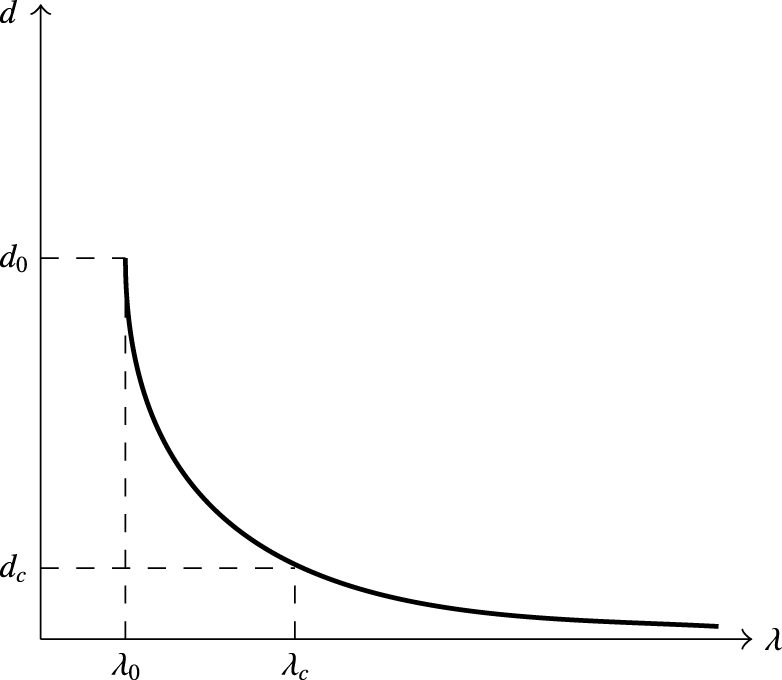
, whereas the function
 $d~(=d(\unicode[STIX]{x1D706}))$
decreases strictly monotonically and tends to zero as
 $\unicode[STIX]{x1D706}\rightarrow +\infty$
(see figure 2). Depending on the behaviour of
 $\unicode[STIX]{x1D6FA}$
on
 $[0,1]$
, the value
 $d_{0}=\lim _{s\rightarrow \unicode[STIX]{x1D706}_{0}+0}d(\unicode[STIX]{x1D706})$
can be finite or infinite (see below). It should be noted that the solution (2.3) is well defined for
 $\unicode[STIX]{x1D706}=\unicode[STIX]{x1D706}_{0}$
when
 $d_{0}<+\infty$
.
A sketch of the graph of
 $d(\unicode[STIX]{x1D706})$
in the case when
 $d_{0}<\infty$
.

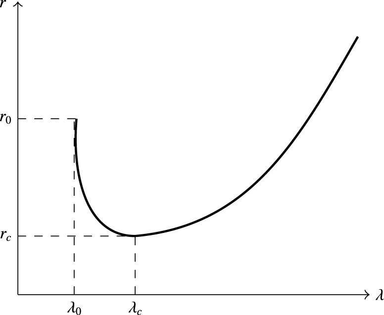
A sketch of the graph of
 ${\mathcal{R}}(\unicode[STIX]{x1D706})$
in the case when
 $d_{0}<\infty$
.

Furthermore, according to the last relation (2.1), the value of
 $\unicode[STIX]{x1D706}$
in (2.3) must be determined from the equation
 $$\begin{eqnarray}r={\mathcal{R}}(\unicode[STIX]{x1D706}),\quad \text{where }{\mathcal{R}}(\unicode[STIX]{x1D706})=[\unicode[STIX]{x1D706}^{2}-2\unicode[STIX]{x1D6FA}(1)+2\,d(\unicode[STIX]{x1D706})]/3.\end{eqnarray}$$
One comes to this conclusion by substituting the first expression (2.3) into the last relation (2.1). It is easy to check that the function
 ${\mathcal{R}}(\unicode[STIX]{x1D706})$
has only one minimum, say
 $r_{c}>0$
, attained at some
 $\unicode[STIX]{x1D706}_{c}>\unicode[STIX]{x1D706}_{0}$
(see figure 3). Hence
 $r_{c}$
is the critical value of
 $r$
in the same sense as
 $r=1$
is critical in the irrotational case, that is, no
 $\unicode[STIX]{x1D706}$
can be found from (2.4) when
 $r<r_{c}$
. It is clear that
 $$\begin{eqnarray}\int _{0}^{1}\frac{\text{d}\unicode[STIX]{x1D70F}}{[\unicode[STIX]{x1D706}_{c}^{2}-2\unicode[STIX]{x1D6FA}(\unicode[STIX]{x1D70F})]^{3/2}}=1,\end{eqnarray}$$
which, in particular, implies that
 $\unicode[STIX]{x1D706}_{c}^{2}-\unicode[STIX]{x1D706}_{0}^{2}\leqslant 1$
.
If
 $d_{0}=+\infty$
, then for every
 $r>r_{c}$
equation (2.4) has two solutions
 $\unicode[STIX]{x1D706}_{+}(r)$
and
 $\unicode[STIX]{x1D706}_{-}(r)$
such that
 $\unicode[STIX]{x1D706}_{0}<\unicode[STIX]{x1D706}_{+}<\unicode[STIX]{x1D706}_{c}<\unicode[STIX]{x1D706}_{-}$
. By substituting
 $\unicode[STIX]{x1D706}_{+}$
and
 $\unicode[STIX]{x1D706}_{-}$
into (2.3), one obtains two stream solutions, say
 $(u_{+},d_{+})$
and
 $(u_{-},d_{-})$
. However, if
 $d_{0}<+\infty$
, then both
 $\unicode[STIX]{x1D706}_{+}$
and
 $\unicode[STIX]{x1D706}_{-}$
, and consequently the corresponding stream solutions satisfying inequality (1.5), exist only for
 $r\in (r_{c},r_{0})$
, where
 $r_{0}={\mathcal{R}}(\unicode[STIX]{x1D706}_{0})$
. It should be noted that
 $d_{0}>d_{+}>d_{c}>d_{-}$
, where
 $d_{c}=d(\unicode[STIX]{x1D706}_{c})$
. The shear flows described by
 $(u_{+},d_{+})$
and
 $(u_{-},d_{-})$
are analogous to the uniform sub- and supercritical flows, respectively, existing in the irrotational case.
It is worth mentioning that the values
 $d_{+}(r)$
and
 $d_{-}(r)$
provide important bounds for wave profiles in the case when a rotational flow is unidirectional; see Kozlov, Kuznetsov & Lokharu (Reference Kozlov, Kuznetsov and Lokharu2015) for the proof. Namely, if
 $r\in (r_{c},r_{0})$
, then the inequalities
 $$\begin{eqnarray}d_{-}(r)<\unicode[STIX]{x1D702}(x)~~\text{for all}~x\in \mathbb{R}\quad \text{and}\quad \inf \unicode[STIX]{x1D702}<d_{+}(r)\leqslant \sup \unicode[STIX]{x1D702}\end{eqnarray}$$
hold for all non-stream solutions. Moreover, the last inequality is strict provided
 $\sup \unicode[STIX]{x1D702}$
is attained at some point. Finally, problem (1.1)–(1.4) has no solution at all if
 $r<r_{c}$
, whereas if
 $r=r_{c}$
, then only the stream solution (2.3) exists.
To analyse the dependence of
 $d_{0}$
on the vorticity distribution, the following three options were considered in Kozlov & Kuznetsov (Reference Kozlov and Kuznetsov2011b
):
-
(i)
$d_{0}=+\infty$
; -
(ii)
$d_{0}<+\infty$
and
$u^{\prime }(0)=0$
,
$u^{\prime }(d_{0})\neq 0$
; -
(iii)
$d_{0}<+\infty$
and
$u^{\prime }(d_{0})=0$
.


Thus, we have that
 $d_{0}<+\infty$
provided either
 $u^{\prime }(0)=0$
or
 $u^{\prime }(d_{0})=0$
. This classification can be reformulated in terms of the vorticity distribution as follows.
-
(i) The value
$\max _{0\leqslant p\leqslant 1}\unicode[STIX]{x1D6FA}(p)$
is attained either at an inner point of
$(0,1)$
or at one (or both) of the end points. In the latter case, either
$\unicode[STIX]{x1D714}(1)=0$
when
$\unicode[STIX]{x1D6FA}(1)>\unicode[STIX]{x1D6FA}(p)$
for
$p\in (0,1)$
or
$\unicode[STIX]{x1D714}(0)=0$
when
$\unicode[STIX]{x1D6FA}(0)>\unicode[STIX]{x1D6FA}(p)$
for
$p\in (0,1)$
(or both of these conditions hold simultaneously). -
(ii) The inequality
$\unicode[STIX]{x1D6FA}(0)>\unicode[STIX]{x1D6FA}(p)$
holds for
$p\in (0,1]$
and
$\unicode[STIX]{x1D714}(0)<0$
. -
(iii) The inequality
$\unicode[STIX]{x1D6FA}(p)<\unicode[STIX]{x1D6FA}(1)$
holds for
$p\in (0,1)$
and
$\unicode[STIX]{x1D714}(1)>0$
. Moreover, if
$\unicode[STIX]{x1D6FA}(1)=0$
, then
$\unicode[STIX]{x1D714}(0)<0$
and
$\unicode[STIX]{x1D714}(1)>0$
must hold simultaneously.


Conditions (i)–(iii) define three disjoint sets of vorticity distributions whose union gives the whole set of distributions that are continuous on
 $[0,1]$
.
2.2 Flow force and the cuspidal region
${\mathcal{C}}_{\unicode[STIX]{x1D714}}$

To the best of the authors’ knowledge, the flow force invariant (see formula (1.7) above) was first considered for rotational waves by Keady & Norbury (Reference Keady and Norbury1978). Up to a slight difference in the definition of
 $\unicode[STIX]{x1D6FA}$
, their expression is as follows (cf. (1.9) expressing the non-dimensional flow force in the irrotational case):
 $$\begin{eqnarray}s=s(\unicode[STIX]{x1D713},\unicode[STIX]{x1D702})=\left[r+\frac{2}{3}\unicode[STIX]{x1D6FA}(1)\right]\unicode[STIX]{x1D702}(x)-\frac{1}{3}\left\{\unicode[STIX]{x1D702}^{2}(x)-\int _{0}^{\unicode[STIX]{x1D702}(x)}[\unicode[STIX]{x1D713}_{y}^{2}-\unicode[STIX]{x1D713}_{x}^{2}-2\unicode[STIX]{x1D6FA}(\unicode[STIX]{x1D713})]\,\text{d}y\right\}.\end{eqnarray}$$
If
 $(\unicode[STIX]{x1D713},\unicode[STIX]{x1D702})$
is a solution of problem (1.1)–(1.4), then it is straightforward to check that this expression is independent of
 $x$
.
By
 $s_{\pm }(r)$
we denote the flow force corresponding to the stream solution
 $(u_{\pm }(y),d_{\pm })$
, and so
 $$\begin{eqnarray}s_{\pm }(r)=\left[r+\frac{2}{3}\unicode[STIX]{x1D6FA}(1)\right]d_{\pm }-\frac{1}{3}\left\{d_{\pm }^{2}-\int _{0}^{d_{\pm }}[(u_{\pm })_{y}^{2}-2\unicode[STIX]{x1D6FA}(u_{\pm })]\,\text{d}y\right\}.\end{eqnarray}$$
It should be noted that the equation
 $s=s_{+}(r)$
 $(s=s_{-}(r))$
gives the upper (lower, respectively) curve bounding the cuspidal region
 ${\mathcal{C}}_{\unicode[STIX]{x1D714}}$
that has its tip at
 $(r_{c},s_{c})$
; here
 $$\begin{eqnarray}s_{c}=s_{-}(r_{c})=s_{+}(r_{c}),\end{eqnarray}$$
in which case
 $d_{c}$
stands in the above formula instead of
 $d_{-}$
and
 $d_{+}$
, respectively. It occurs that the curve
 $s=s_{-}(r)$
always goes to infinity, being defined for all
 $r\in [r_{c},+\infty )$
, whereas
 $s=s_{+}(r)$
goes to infinity only when
 $r_{0}=+\infty$
or, what is the same, condition (i) holds for the vorticity distribution. Thus, the cuspidal region
 ${\mathcal{C}}_{\unicode[STIX]{x1D714}}$
is similar to
 ${\mathcal{C}}$
in this case. On the contrary, if
 $\unicode[STIX]{x1D714}$
satisfies either condition (ii) or condition (iii), then both
 $d_{0}$
and
 $r_{0}$
are finite, and so the curve
 $s=s_{+}(r)$
terminates at the point
 $(r_{0},s_{+}(r_{0}))$
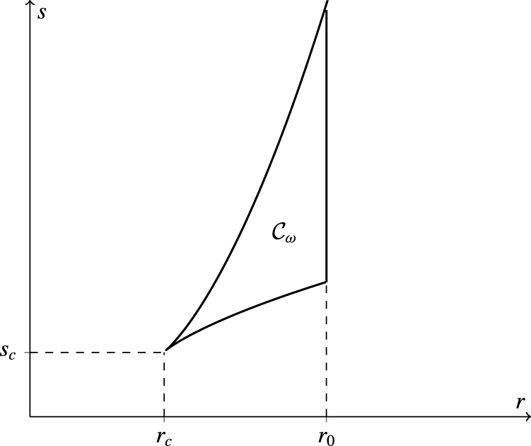
. Hence the region
 ${\mathcal{C}}_{\unicode[STIX]{x1D714}}$
is bounded under these conditions and
 $\unicode[STIX]{x2202}{\mathcal{C}}_{\unicode[STIX]{x1D714}}$
consists of two arcs and the segment that connects them and lies on the line
 $r=r_{0}$
(see figure 4).
A sketch of the region
 ${\mathcal{C}}_{\unicode[STIX]{x1D714}}$
corresponding to a vorticity distribution with finite
 $r_{0}$
.

2.3 Definitions and formulations
Since we study waves only for near-critical values of
 $r$
, it is convenient to assume that
 $$\begin{eqnarray}r\leqslant {\mathcal{R}}((\unicode[STIX]{x1D706}_{c}+\unicode[STIX]{x1D706}_{0})/2).\end{eqnarray}$$
Also, the following notation will be used below:
 $$\begin{eqnarray}\unicode[STIX]{x1D714}_{0}=\max _{[0,1]}|\unicode[STIX]{x1D714}|,\quad \unicode[STIX]{x1D714}_{1}=\unicode[STIX]{x1D714}_{0}+\text{ess}\,\text{sup}_{[0,1]}|\unicode[STIX]{x1D714}^{\prime }|.\end{eqnarray}$$
Let us specify the problem that we investigate in what follows.
Definition 1. Let
 $\unicode[STIX]{x1D714}$
be a Lipschitz vorticity distribution. We say that
 $(\unicode[STIX]{x1D713},\unicode[STIX]{x1D702})$
belonging to
 $C_{loc}^{1}(\bar{D})\times W^{1,\infty }(\mathbb{R})$
is a solution of problem
 $P_{r}^{M}$
for some
 $M>0$
and
 $r>r_{c}$
(
 $r_{c}>0$
is the critical value of Bernoulli’s constant for
 $\unicode[STIX]{x1D714}$
), when the following conditions are fulfilled. The inequality
 $|\unicode[STIX]{x1D702}^{\prime }(x)|\leqslant M$
is true almost everywhere on
 $\mathbb{R}$
, whereas inequality (1.5) holds for
 $\unicode[STIX]{x1D713}$
that satisfies (1.1) in a weak sense and the boundary conditions (1.2)–(1.4) are valid pointwise.
Let us formulate our main results concerning problem
 $P_{r}^{M}$
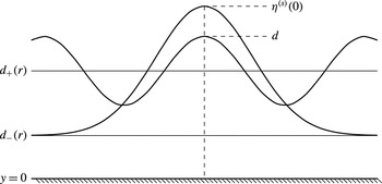
. Our first theorem provides a complete description of the set of waves existing in the near-critical regime; these are the family of Stokes waves and a solitary wave naturally parametrised by their heights at the crest (see figure 5).
Theorem 1. For every positive
 $M$
there exists
 $r^{\prime }\in (r_{c},r_{0})$
(depending also on
 $\unicode[STIX]{x1D714}_{1}$
) such that the following assertions are true.
-
(I) For every
$r\in (r_{c},r^{\prime }]$
problem
$P_{r}^{M}$
has one and only one solitary-wave solution
$(\unicode[STIX]{x1D713}^{(s)},\unicode[STIX]{x1D702}^{(s)})$
such that
$\unicode[STIX]{x1D702}^{(s)}$
is an even function. All other solitary-wave solutions are horizontal translations of
$(\unicode[STIX]{x1D713}^{(s)},\unicode[STIX]{x1D702}^{(s)})$
. -
(II) If
$(\unicode[STIX]{x1D713},\unicode[STIX]{x1D702})$
is a Stokes-wave solution of problem
$P_{r}^{M}$
with
$r\in (r_{c},r^{\prime }]$
, then the following inequalities hold, (2.12)where
$$\begin{eqnarray}d_{+}=d(\unicode[STIX]{x1D706}_{+}(r))<\max _{x\in \mathbb{R}}\unicode[STIX]{x1D702}(x)<\unicode[STIX]{x1D702}^{(s)}(0),\end{eqnarray}$$
$d(\unicode[STIX]{x1D706})$
is defined by the second formula (2.3) and
$\unicode[STIX]{x1D706}_{+}(r)$
is the smallest root of (2.4).
-
(III) For every
$r\in (r_{c},r^{\prime }]$
and every
$d\in (d_{+},\unicode[STIX]{x1D702}^{(s)}(0))$
problem
$P_{r}^{M}$
has one and only one Stokes-wave solution
$(\unicode[STIX]{x1D713},\unicode[STIX]{x1D702})$
such that (2.13)Thus, the family of Stokes waves with crests on the
$$\begin{eqnarray}\max _{x\in \mathbb{R}}\unicode[STIX]{x1D702}(x)=\unicode[STIX]{x1D702}(0)=d.\end{eqnarray}$$
$y$
-axis is parametrised by
$d$
. All other Stokes-wave solutions are horizontal translations of
$(\unicode[STIX]{x1D713},\unicode[STIX]{x1D702})$
.
-
(IV) For every
$r\in (r_{c},r^{\prime }]$
all solutions of problem
$P_{r}^{M}$
are exhausted by those described in assertions (I) and (III) and stream solutions.


A sketch of the hierarchy of waves corresponding to a near-critical value of
 $r$
.

In formula (2.12), the inequality on the left-hand side was proved earlier (see Kozlov et al. Reference Kozlov, Kuznetsov and Lokharu2015), and it is included for the sake of completeness. In the next assertion, we deal with the question about the continuity of waves considered in theorem 1. It is shown that all these waves depend continuously on their depths at the crest, but in a certain integral sense.
Theorem 2. For every positive
 $M$
there exists
 $r^{\prime \prime }\in (r_{c},r_{0})$
(depending also on
 $\unicode[STIX]{x1D714}_{1}$
) such that any two solutions of problem
 $P_{r}^{M}$
with
 $r\in (r_{c},r^{\prime \prime }]$
, say
 $(\unicode[STIX]{x1D713}^{(1)},\unicode[STIX]{x1D702}^{(1)})$
and
 $(\unicode[STIX]{x1D713}^{(2)},\unicode[STIX]{x1D702}^{(2)})$
, satisfy the inequality
 $$\begin{eqnarray}\int _{\mathbb{R}}|\unicode[STIX]{x1D702}^{(1)}(x)-\unicode[STIX]{x1D702}^{(2)}(x)|^{2}\,\text{e}^{-\unicode[STIX]{x1D703}|x-x_{0}|}\,\text{d}x\leqslant C[|\unicode[STIX]{x1D702}^{(1)}(x_{0})-\unicode[STIX]{x1D702}^{(2)}(x_{0})|^{2}+|\unicode[STIX]{x1D702}_{x}^{(1)}(x_{0})-\unicode[STIX]{x1D702}_{x}^{(2)}(x_{0})|^{2}],\end{eqnarray}$$
where the constants
 $C$
and
 $\unicode[STIX]{x1D703}$
depend only on
 $\unicode[STIX]{x1D714}_{0}$
and
 $x_{0}\in \mathbb{R}$
is arbitrary.
Theorems 1 and 2 are analogous to theorems 2.1 and 2.2, respectively, proved by Kozlov & Kuznetsov (Reference Kozlov and Kuznetsov2010). In the latter paper, the mentioned theorems provided the basis for verification of assertions (1) and (2) of the Benjamin–Lighthill conjecture for irrotational waves. Here, theorems 1 and 2 serve for the same purpose for waves with vorticity (see § 6 below), but our techniques used for establishing these theorems differ radically from those applied in Kozlov & Kuznetsov (Reference Kozlov and Kuznetsov2010).
Let
 $r^{\prime }\in (r_{c},r_{0})$
be the value of Bernoulli’s constant from theorem 1. By
 ${\mathcal{P}}_{r}^{M}$
with
 $r\in (r_{c},r^{\prime }]$
we denote the set of solutions to problem
 $P_{r}^{M}$
that have the following property. The second component
 $\unicode[STIX]{x1D702}$
has one of its crests on the
 $y$
-axis (see assertions (I) and (III) of theorem 1 and figure 5). Then formula (2.7) defines the following mapping:
 $$\begin{eqnarray}{\mathcal{P}}_{r}^{M}\ni (\unicode[STIX]{x1D713},\unicode[STIX]{x1D702})\mapsto s\in [\!s_{-}(r),s_{+}(r)\!)\!.\end{eqnarray}$$
The last of our main results concerns this mapping; namely, the set
 ${\mathcal{P}}_{r}^{M}$
is parametrised by the flow force
 $s$
which is an alternative parametrisation to that in theorem 1.
Theorem 3. For every positive
 $M$
there exists
 $r^{\prime \prime \prime }\in (r_{c},r_{0})$
(depending also on
 $\unicode[STIX]{x1D714}_{1}$
) such that for every
 $r\in (r_{c},r^{\prime \prime \prime }]$
mapping (2.15) is one-to-one.
This theorem shows that for the family of waves having their crests on the
 $y$
-axis there exists the parametrisation in terms of
 $s$
, which is alternative to that described in assertion (III) of theorem 1. Also, theorem 3 allows us to verify assertion (3) of the Benjamin–Lighthill conjecture for near-critical rotational waves; irrotational ones are included as a particular case with zero vorticity.
It will follow from our proofs of theorems 2 and 3 that
 $r^{\prime \prime }\geqslant r^{\prime }=r^{\prime \prime \prime }$
.
2.4 Proof strategy
Here we outline our approach to proving theorems 1–3. The first crucial step is made in § 4, where properties of solutions to problem
 $P_{r}^{M}$
are studied. We begin with a uniform bound for
 $\unicode[STIX]{x1D735}\unicode[STIX]{x1D713}$
that depends only on
 $\unicode[STIX]{x1D714}_{0}$
in the case when Bernoulli’s constant is separated from
 $r_{0}$
. Then we show that
 $\unicode[STIX]{x1D702}-d_{+}(r)$
is arbitrarily small if
 $r$
is sufficiently close to
 $r_{c}$
. In the proof of this assertion, we use the problem’s reformulation based on the partial hodograph transform introduced in § 3. Finally, bounds for
 $C^{2,\unicode[STIX]{x1D6FC}}$
norms of
 $\unicode[STIX]{x1D713}$
and
 $\unicode[STIX]{x1D702}$
are obtained for some
 $\unicode[STIX]{x1D6FC}\in (0,1)$
and the assumption that the positive
 $\unicode[STIX]{x1D713}_{y}$
is separated from zero is essential.
The fact that near-critical waves are of small amplitude allows us to apply results of Groves & Wahlén (Reference Groves and Wahlén2008), according to which all these waves are exhausted by a continuous branch of Stokes waves bifurcating from a horizontal shear flow and terminating by the solitary wave of elevation. In § 6 we combine this assertion and theorem 2, independently proved in § 5, and conclude that these waves are uniquely parametrised by height at the crest; to be specific, the latter is supposed to lie on the
 $y$
-axis. This completes the proof of theorem 1.
The second crucial step is the proof of theorem 5 in § 5. This theorem (it is a slightly stronger form of theorem 2) deals with the unknown function
 $h$
arising in the problem’s transformation considered in § 3, but its proof is based on another equivalent formulation of the problem proposed by Groves & Wahlén (Reference Groves and Wahlén2008). An essential point is the spectral splitting procedure applied to the spectral problem related to the system linearised near a stream solution. Its combination with several rather sophisticated estimates completes the proof of theorem 5.
Finally, we express the flow force in terms of specially parametrised function
 $h$
(see § 6) in order to prove theorem 3. The derivative of the flow force with respect to the parameter we evaluate with the help of estimates obtained in § 5, thus demonstrating the monotonicity of the flow force, and this completes verification of the Benjamin–Lighthill conjecture for the near-critical regime.
3 Partial hodograph transform and an auxiliary spectral problem
In our proofs, we use an equivalent statement of the problem. Its advantage is that it is posed in the fixed strip
 $S=\mathbb{R}\times (0,1)$
instead of the unknown domain
 $D$
in the original problem (1.1)–(1.5). The last condition is essential because reformulation is possible only for unidirectional flows. The corresponding change of variables was proposed by Dubreil-Jacotin (Reference Dubreil-Jacotin1934); it is referred to as the partial hodograph transform (see § 3.1) to distinguish it from the classical hodograph transform used in Kozlov & Kuznetsov (Reference Kozlov and Kuznetsov2010) for justification of the Benjamin–Lighthill conjecture for near-critical, irrotational waves. In §§ 3.2 and 3.3, we investigate an auxiliary spectral problem related to the linearisation of the reformulated problem. This Sturm–Liouville problem was considered earlier, for example, by Constantin & Strauss (Reference Constantin and Strauss2011). However, to the best of our knowledge, the estimates of its eigenvalues and eigenfunctions (they are obtained in § 3.3 and used in the proof of our main results) are new.
3.1 Partial hodograph transform
Inequality (1.5) and the boundary conditions (1.2) and (1.3) allow us to put
 $q=x$
and
 $p=\unicode[STIX]{x1D713}(x,y)$
, thus mapping
 $D\ni (x,y)\mapsto (q,p)\in S=\mathbb{R}\times (0,1)$
. Considering
 $(q,p)$
as independent variables in
 $S$
, we use
 $y$
as the new unknown function for which
 $h(q,p)$
is the standard notation. A straightforward calculation shows that
 $$\begin{eqnarray}h_{q}=-\frac{\unicode[STIX]{x1D713}_{x}}{\unicode[STIX]{x1D713}_{y}}\quad \text{and}\quad h_{p}=\frac{1}{\unicode[STIX]{x1D713}_{y}},\end{eqnarray}$$
thus yielding that problem (1.1)–(1.4) takes the following form in terms of new variables:
 $$\begin{eqnarray}\displaystyle & \displaystyle \left[\frac{h_{q}}{h_{p}}\right]_{q}-\frac{1}{2}\left[\frac{1+h_{q}^{2}}{h_{p}^{2}}\right]_{p}-\unicode[STIX]{x1D714}(p)=0,\quad (q,p)\in S, & \displaystyle\end{eqnarray}$$
 $$\begin{eqnarray}\displaystyle & \displaystyle h(0,q)=0,\quad q\in \mathbb{R}, & \displaystyle\end{eqnarray}$$
 $$\begin{eqnarray}\displaystyle & \displaystyle \frac{1+h_{q}^{2}}{h_{p}^{2}}=3r-2h,\quad p=1,~q\in \mathbb{R}. & \displaystyle\end{eqnarray}$$
On the other hand, noting that
 $$\begin{eqnarray}\unicode[STIX]{x1D713}_{x}=-\frac{h_{q}}{h_{p}}\quad \text{and}\quad \unicode[STIX]{x1D713}_{y}=\frac{1}{h_{p}},\end{eqnarray}$$
one recovers the velocity field in
 $\bar{D}$
which is
 $(\unicode[STIX]{x1D713}_{y},-\unicode[STIX]{x1D713}_{x})$
. Besides, the free surface profile is given by the equality
 $\unicode[STIX]{x1D702}(x)=h(x,1)$
, where
 $x\in \mathbb{R}$
.
The second advantage of relations (3.2)–(3.4) compared with (1.1)–(1.4), to which they are equivalent under reasonable smoothness assumptions (see Constantin & Strauss (Reference Constantin and Strauss2011) for a detailed account), is that only one unknown function
 $h$
is involved.
In terms of problem (3.2)–(3.4), a stream solution is a single function, say
 $H(p,\unicode[STIX]{x1D706})$
, which has the following form:
 $$\begin{eqnarray}H(p,\unicode[STIX]{x1D706})=\int _{0}^{p}\frac{\text{d}\unicode[STIX]{x1D70F}}{\sqrt{\unicode[STIX]{x1D706}^{2}-2\unicode[STIX]{x1D6FA}(\unicode[STIX]{x1D70F})}}.\end{eqnarray}$$
Here
 $\unicode[STIX]{x1D706}\in (\unicode[STIX]{x1D706}_{c},\unicode[STIX]{x1D706}_{0}]$
is the same parameter as in (2.3) and (2.4), whereas
 $d_{\pm }(r)=H(1,\unicode[STIX]{x1D706}_{\pm }(r))$
.
3.2 Auxiliary Sturm–Liouville problem
It is straightforward to check that, linearising (3.2) near the stream solution
 $H$
, one obtains an equation that involves the operator
 $-\unicode[STIX]{x2202}_{p}(H_{p}^{-3}\unicode[STIX]{x2202}_{p})$
. This is the reason to consider the following Sturm–Liouville problem:
 $$\begin{eqnarray}\displaystyle & \displaystyle -\!\left[\frac{\unicode[STIX]{x1D719}_{p}}{H_{p}^{3}}\right]_{p}=\unicode[STIX]{x1D707}\frac{\unicode[STIX]{x1D719}}{H_{p}},\quad p\in (0,1), & \displaystyle\end{eqnarray}$$
 $$\begin{eqnarray}\displaystyle & \displaystyle \unicode[STIX]{x1D719}_{p}(1)=H_{p}^{3}(1)\unicode[STIX]{x1D719}(1), & \displaystyle\end{eqnarray}$$
 $$\begin{eqnarray}\displaystyle & \displaystyle \unicode[STIX]{x1D719}(0)=0, & \displaystyle\end{eqnarray}$$
where
 $\unicode[STIX]{x1D707}$
is the spectral parameter. However, the eigenvalues and eigenfunctions of this problem depend also on
 $\unicode[STIX]{x1D706}$
because
 $H$
depends on it.
The spectrum of (3.7)–(3.9), which we denote by
 $\{\unicode[STIX]{x1D707}_{k}\}_{k=0}^{+\infty }$
, is essential in our study of problem (3.2)–(3.4). All eigenvalues are simple, that is,
 $$\begin{eqnarray}\unicode[STIX]{x1D707}_{0}<\unicode[STIX]{x1D707}_{1}<\cdots <\unicode[STIX]{x1D707}_{n}<\cdots \,,\end{eqnarray}$$
where
 $\unicode[STIX]{x1D707}_{0}$
may be either positive or negative.
3.2.1 A preliminary estimate of
$\unicode[STIX]{x1D707}_{1}$

Let us show that
 $$\begin{eqnarray}\unicode[STIX]{x1D707}_{1}\geqslant \unicode[STIX]{x03C0}^{2}\frac{\mathfrak{m}}{\mathfrak{M}^{3}},\end{eqnarray}$$
where
 $$\begin{eqnarray}\mathfrak{M}=\max _{p\in [0,1]}H_{p}=(\unicode[STIX]{x1D706}^{2}-\unicode[STIX]{x1D706}_{0}^{2})^{-1/2}\quad \text{and}\quad \mathfrak{m}=\min _{p\in [0,1]}H_{p}=\left[\unicode[STIX]{x1D706}^{2}-2\min _{\unicode[STIX]{x1D70F}\in [0,1]}\unicode[STIX]{x1D6FA}(\unicode[STIX]{x1D70F})\right]^{-1/2}.\end{eqnarray}$$
Indeed, it is well known that the smallest eigenvalue of the operator
 $-\text{d}^{2}/\text{d}p^{2}$
on
 $(0,1)$
with the Dirichlet boundary conditions is
 $$\begin{eqnarray}\inf _{\unicode[STIX]{x1D719}\in W_{0}^{1,2}(0,1)}\frac{\displaystyle \int _{0}^{1}\unicode[STIX]{x1D719}_{p}^{2}\,\text{d}p}{\displaystyle \int _{0}^{1}\unicode[STIX]{x1D719}^{2}\,\text{d}p}=\unicode[STIX]{x03C0}^{2}.\end{eqnarray}$$
Since the fundamental eigenfunction
 $\unicode[STIX]{x1D719}_{0}$
of problem (3.7)–(3.9) is non-negative irrespective of the sign of the corresponding eigenvalue
 $\unicode[STIX]{x1D707}_{0}$
, the eigenfunction
 $\unicode[STIX]{x1D719}_{1}$
has exactly one zero, say
 $p_{\ast }\in (0,1)$
. Therefore, we have
 $$\begin{eqnarray}\unicode[STIX]{x03C0}^{2}\leqslant p_{\ast }^{2}\frac{\displaystyle \int _{0}^{p_{\ast }}\unicode[STIX]{x1D719}_{1p}^{2}\,\text{d}p}{\displaystyle \int _{0}^{p_{\ast }}\unicode[STIX]{x1D719}_{1p}^{2}\,\text{d}p}\leqslant \frac{\mathfrak{M}^{3}}{\mathfrak{m}}\frac{\displaystyle \int _{0}^{p_{\ast }}\unicode[STIX]{x1D719}_{1p}^{2}H_{p}^{-3}\,\text{d}p}{\displaystyle \int _{0}^{p_{\ast }}\unicode[STIX]{x1D719}_{1}^{2}H_{p}^{-1}\,\text{d}p}\leqslant \frac{\mathfrak{M}^{3}}{\mathfrak{m}}\unicode[STIX]{x1D707}_{1},\end{eqnarray}$$
which yields inequality (3.11).
3.2.2 Properties of
$\unicode[STIX]{x1D707}_{0}$
and
$\unicode[STIX]{x1D719}_{0}$


Let us consider the initial value problem
 $$\begin{eqnarray}-(H_{p}^{-3}V_{p})_{p}=\unicode[STIX]{x1D707}H_{p}^{-1}V,\quad V(0)=0,\quad V_{p}(0)=1,\end{eqnarray}$$
depending on the parameters
 $\unicode[STIX]{x1D707}$
and
 $\unicode[STIX]{x1D706}$
(the latter is involved through
 $H$
), and so we will write
 $V(p;\unicode[STIX]{x1D706},\unicode[STIX]{x1D707})$
when necessary. It should be noted that
 $V$
is a monotonic function of
 $p\in [0,1]$
which depends analytically on
 $\unicode[STIX]{x1D706}>\unicode[STIX]{x1D706}_{0}$
and
 $\unicode[STIX]{x1D707}\in \mathbb{R}$
. In terms of
 $V$
, the eigenvalue
 $\unicode[STIX]{x1D707}_{0}=\unicode[STIX]{x1D707}_{0}(\unicode[STIX]{x1D706})$
is equal to the least root of the equation
 $\unicode[STIX]{x1D70E}(\unicode[STIX]{x1D706},\unicode[STIX]{x1D707})=0$
, where
 $$\begin{eqnarray}\unicode[STIX]{x1D70E}(\unicode[STIX]{x1D706},\unicode[STIX]{x1D707})=[H_{p}(1,\unicode[STIX]{x1D706})]^{-3}V_{p}(1;\unicode[STIX]{x1D706},\unicode[STIX]{x1D707})-V(1;\unicode[STIX]{x1D706},\unicode[STIX]{x1D707})\end{eqnarray}$$
depends on
 $\unicode[STIX]{x1D706}>\unicode[STIX]{x1D706}_{0}$
and
 $\unicode[STIX]{x1D707}\in \mathbb{R}$
analytically. Moreover, the eigenfunction
 $\unicode[STIX]{x1D719}_{0}$
corresponding to
 $\unicode[STIX]{x1D707}_{0}$
is equal to
 $V(p;\unicode[STIX]{x1D706},\unicode[STIX]{x1D707}_{0})$
, that is, it solves (3.15) for
 $\unicode[STIX]{x1D707}=\unicode[STIX]{x1D707}_{0}$
.
In order to find the derivative
 $\unicode[STIX]{x1D70E}_{\unicode[STIX]{x1D707}}$
, it is convenient to differentiate the first equality (3.15) with respect to
 $\unicode[STIX]{x1D707}$
, then multiply the result by
 $V$
and integrate over
 $(0,1)$
. Thus we obtain after integration by parts that
 $$\begin{eqnarray}\unicode[STIX]{x1D70E}_{\unicode[STIX]{x1D707}}(\unicode[STIX]{x1D706},\unicode[STIX]{x1D707})=\frac{-1}{V(1;\unicode[STIX]{x1D706},\unicode[STIX]{x1D707})}\int _{0}^{1}\frac{V^{2}(p;\unicode[STIX]{x1D706},\unicode[STIX]{x1D707})}{H_{p}(p,\unicode[STIX]{x1D706})}\,\text{d}p.\end{eqnarray}$$
Hence
 $\unicode[STIX]{x1D70E}_{\unicode[STIX]{x1D707}}$
is always negative, which implies that
 $\unicode[STIX]{x1D70E}(\unicode[STIX]{x1D706},\unicode[STIX]{x1D707})>0$
when
 $\unicode[STIX]{x1D707}<\unicode[STIX]{x1D707}_{0}(\unicode[STIX]{x1D706})$
.
Furthermore, if
 $\unicode[STIX]{x1D707}=0$
, then
 $V(p;\unicode[STIX]{x1D706},0)=-\unicode[STIX]{x1D706}^{2}\unicode[STIX]{x2202}_{\unicode[STIX]{x1D706}}H(p,\unicode[STIX]{x1D706})$
, and so
 $$\begin{eqnarray}\unicode[STIX]{x1D70E}(\unicode[STIX]{x1D706},0)=\unicode[STIX]{x1D706}^{2}\unicode[STIX]{x2202}_{\unicode[STIX]{x1D706}}\left[\frac{1}{2H_{p}^{2}(1,\unicode[STIX]{x1D706})}+H(1,\unicode[STIX]{x1D706})\right]=\frac{3\unicode[STIX]{x1D706}^{2}}{2}{\mathcal{R}}^{\prime }(\unicode[STIX]{x1D706}),\end{eqnarray}$$
where the last equality is a consequence of the definitions of
 $H$
and
 ${\mathcal{R}}$
(see (3.6) and (2.4), respectively). Since
 ${\mathcal{R}}^{\prime }(\unicode[STIX]{x1D706})$
is negative for
 $\unicode[STIX]{x1D706}<\unicode[STIX]{x1D706}_{c}$
and positive for
 $\unicode[STIX]{x1D706}>\unicode[STIX]{x1D706}_{c}$
(see figure 2), it follows from (3.18) and (3.17) that
 $\unicode[STIX]{x1D707}_{0}(\unicode[STIX]{x1D706})$
is positive (negative) for
 $\unicode[STIX]{x1D706}>\unicode[STIX]{x1D706}_{c}$
(
 $\unicode[STIX]{x1D706}<\unicode[STIX]{x1D706}_{c}$
, respectively) and
 $\unicode[STIX]{x1D707}_{0}(\unicode[STIX]{x1D706}_{c})=0$
.
Let us estimate
 $|\unicode[STIX]{x1D707}_{0}(\unicode[STIX]{x1D706})|$
for
 $\unicode[STIX]{x1D706}<\unicode[STIX]{x1D706}_{c}$
when
 $\unicode[STIX]{x1D707}_{0}(\unicode[STIX]{x1D706})<0$
for which we have
 $$\begin{eqnarray}\unicode[STIX]{x1D707}_{0}=\min _{v\in W_{0}^{1,2}(0,1)}\frac{\displaystyle \int _{0}^{1}v^{2}H_{p}^{-3}\,\text{d}p-v^{2}(1)}{\displaystyle \int _{0}^{1}v^{2}H_{p}^{-1}\,\text{d}p}\geqslant \min _{v\in W_{0}^{1,2}(0,1)}\frac{\displaystyle \mathfrak{M}^{-3}\int _{0}^{1}v^{2}\,\text{d}p-v^{2}(1)}{\displaystyle \mathfrak{m}^{-1}\int _{0}^{1}v^{2}\,\text{d}p},\end{eqnarray}$$
where
 $\mathfrak{M}$
and
 $\mathfrak{m}$
are the same as in (3.11). The last minimum is equal to the fundamental eigenvalue of the problem with constant coefficients obtained by changing
 $H_{p}$
to
 $\mathfrak{M}$
in (3.7)–(3.9). This minimum is
 $-\unicode[STIX]{x1D705}^{2}\mathfrak{m}\mathfrak{M}^{-3}$
, where
 $\unicode[STIX]{x1D705}=\unicode[STIX]{x1D705}(\mathfrak{M})$
is a root of the equation
 $$\begin{eqnarray}\frac{\sinh \unicode[STIX]{x1D705}}{\unicode[STIX]{x1D705}\cosh \unicode[STIX]{x1D705}}=\frac{1}{\mathfrak{M}^{3}}.\end{eqnarray}$$
Since
 $\mathfrak{M}^{3}\geqslant \int _{0}^{1}H_{p}^{3}\,\text{d}p>1$
, this equation is uniquely solvable and we arrive at the following estimate:
 $$\begin{eqnarray}|\unicode[STIX]{x1D707}_{0}|\leqslant [\unicode[STIX]{x1D705}(\mathfrak{M})]^{2}/\mathfrak{M}^{2}.\end{eqnarray}$$
The variational formulation of (3.2)–(3.4) yields that the right-hand side of the last inequality is a monotonic function of
 $\mathfrak{M}$
.
Now, we turn to estimates of
 $V$
and
 $V_{p}$
. Integrating (3.15) and using the second boundary condition, we obtain that
 $$\begin{eqnarray}V_{p}(p)=\frac{H_{p}^{3}(p)}{\unicode[STIX]{x1D706}^{3}}+|\unicode[STIX]{x1D707}|H_{p}^{3}(p)\int _{0}^{p}\frac{V(p^{\prime })}{H_{p}(p^{\prime })}\,\text{d}p^{\prime },\end{eqnarray}$$
which gives the following lower estimates:
 $$\begin{eqnarray}V(p)\geqslant \frac{p\,\mathfrak{m}^{3}}{\unicode[STIX]{x1D706}^{3}}\quad \text{and}\quad V_{p}(p)\geqslant \frac{\mathfrak{m}^{3}}{\unicode[STIX]{x1D706}^{3}}.\end{eqnarray}$$
To obtain an upper estimate for
 $V$
we integrate (3.22), thus reducing it to an integral equation with a positive operator. Its upper solution gives the required estimate of
 $V$
, and one obtains such a solution using problem (3.7)–(3.9) with
 $H_{p}^{-3}$
and
 $H_{p}^{-1}$
changed to
 $\mathfrak{M}^{-3}$
and
 $\mathfrak{m}^{-1}$
, respectively. This leads to the following inequality:
 $$\begin{eqnarray}V\leqslant \frac{\sinh (\unicode[STIX]{x1D703}p)}{\unicode[STIX]{x1D703}},\quad \text{where }\unicode[STIX]{x1D703}^{2}=|\unicode[STIX]{x1D707}|\frac{\mathfrak{M}^{3}}{\mathfrak{m}}.\end{eqnarray}$$
Combining this and (3.22), we see that
 $$\begin{eqnarray}V_{p}\leqslant \frac{\mathfrak{M}^{3}}{\unicode[STIX]{x1D706}^{3}}+|\unicode[STIX]{x1D707}|\frac{\mathfrak{M}^{3}}{\mathfrak{m}}\int _{0}^{p}\frac{\sinh (\unicode[STIX]{x1D703}p)}{\unicode[STIX]{x1D703}}\,\text{d}p.\end{eqnarray}$$
Let us estimate
 $\unicode[STIX]{x1D707}_{0}^{\prime }(\unicode[STIX]{x1D706})$
, for which purpose we differentiate (3.15) with respect to
 $\unicode[STIX]{x1D706}$
, multiply the result by
 $V$
and integrate the product over
 $(0,1)$
. Thus, after integration by parts we arrive at the following formula:
 $$\begin{eqnarray}\unicode[STIX]{x1D70E}_{\unicode[STIX]{x1D706}}(\unicode[STIX]{x1D706},\unicode[STIX]{x1D707})=\frac{1}{V(1;\unicode[STIX]{x1D706},\unicode[STIX]{x1D707})}\left(\int _{0}^{1}V_{p}^{2}\unicode[STIX]{x2202}_{\unicode[STIX]{x1D706}}H_{p}^{-3}\,\text{d}p-\unicode[STIX]{x1D707}\int _{0}^{1}V^{2}\unicode[STIX]{x2202}_{\unicode[STIX]{x1D706}}H_{p}^{-1}\,\text{d}p\right).\end{eqnarray}$$
Since
 $\unicode[STIX]{x1D707}_{0}^{\prime }(\unicode[STIX]{x1D706})=-\unicode[STIX]{x1D70E}_{\unicode[STIX]{x1D706}}(\unicode[STIX]{x1D706},\unicode[STIX]{x1D707}(\unicode[STIX]{x1D706}))/\unicode[STIX]{x1D70E}_{\unicode[STIX]{x1D707}}(\unicode[STIX]{x1D706},\unicode[STIX]{x1D707}(\unicode[STIX]{x1D706}))$
, relations (3.17) and (3.26) yield that
 $\unicode[STIX]{x1D707}(\unicode[STIX]{x1D706})$
is a Lipschitz function on every interval separated from
 $\unicode[STIX]{x1D706}_{0}$
.
3.3 Estimates for near-critical values of
$r$

In this section, we refine the estimates obtained in §§ 3.1 and 3.2 by applying the assumption (2.10); we recall that this means that
 $\unicode[STIX]{x1D706}\in [(\unicode[STIX]{x1D706}_{0}+\unicode[STIX]{x1D706}_{c})/2,\unicode[STIX]{x1D706}_{c})$
.
Proposition 1. If
 $\unicode[STIX]{x1D706}\in [(\unicode[STIX]{x1D706}_{0}+\unicode[STIX]{x1D706}_{c})/2,\unicode[STIX]{x1D706}_{c})$
, then the following inequalities are valid:
-
(i)
$\unicode[STIX]{x1D707}_{0}(\unicode[STIX]{x1D706})<0$
and
$|\unicode[STIX]{x1D707}_{0}(\unicode[STIX]{x1D706})|\leqslant C_{1}|\unicode[STIX]{x1D706}-\unicode[STIX]{x1D706}_{c}|$
, -
(ii)
$\unicode[STIX]{x1D707}_{1}(\unicode[STIX]{x1D706})\geqslant C_{2}$
, -
(iii)
$C_{3}p\leqslant V(p)\leqslant C_{4}p$
and
$C_{5}\leqslant V_{p}(p)\leqslant C_{6}$
for
$p\in [0,1]$
.






The positive constants
 $C_{1},\ldots ,C_{6}$
depend only on
 $\unicode[STIX]{x1D714}_{0}$
(see the first formula (2.11) for its definition).
Proof. Since the right-hand side terms in (3.11), (3.21) and (3.23)–(3.25) depend monotonically on both
 $\mathfrak{m}$
and
 $\mathfrak{M}$
, the listed estimates imply that (i)–(iii) follow from the inequalities
 $$\begin{eqnarray}C^{\prime }(\unicode[STIX]{x1D714}_{0})\leqslant \unicode[STIX]{x1D706}_{c}\leqslant C^{\prime \prime }(\unicode[STIX]{x1D714}_{0})\end{eqnarray}$$
provided
 $$\begin{eqnarray}\mathfrak{m}\geqslant \mathfrak{m}_{\ast }\quad \text{and}\quad \mathfrak{M}\leqslant \mathfrak{M}_{\ast },\end{eqnarray}$$
where
 $\mathfrak{m}_{\ast }$
and
 $\mathfrak{M}_{\ast }$
are positive constants depending only on
 $\unicode[STIX]{x1D714}_{0}$
.
The definition of
 $\unicode[STIX]{x1D706}_{c}$
implies that
 $\unicode[STIX]{x1D706}_{c}^{2}-\unicode[STIX]{x1D706}_{0}^{2}\leqslant 1$
, which gives the first bound (3.28):
 $$\begin{eqnarray}\mathfrak{m}\geqslant \left[\unicode[STIX]{x1D706}_{c}^{2}-\unicode[STIX]{x1D706}_{0}^{2}+\unicode[STIX]{x1D706}_{0}^{2}-2\min _{\unicode[STIX]{x1D70F}\in [0,1]}\unicode[STIX]{x1D6FA}(\unicode[STIX]{x1D70F})\right]^{-1/2}\geqslant \frac{1}{\sqrt{1+4\,\unicode[STIX]{x1D714}_{0}}}.\end{eqnarray}$$
Furthermore, we have that
 $$\begin{eqnarray}\mathfrak{M}\leqslant \frac{2}{\sqrt{\unicode[STIX]{x1D706}_{c}^{2}-\unicode[STIX]{x1D706}_{0}^{2}}},\end{eqnarray}$$
and so estimating
 $\unicode[STIX]{x1D706}_{c}^{2}-\unicode[STIX]{x1D706}_{0}^{2}$
from below, one obtains the second bound (3.28).
Let
 $\unicode[STIX]{x1D70F}_{0}$
be such that
 $2\unicode[STIX]{x1D6FA}(\unicode[STIX]{x1D70F}_{0})=\unicode[STIX]{x1D706}_{0}^{2}$
, then we have
 $$\begin{eqnarray}\int _{0}^{1}(\unicode[STIX]{x1D706}_{c}^{2}-\unicode[STIX]{x1D706}_{0}^{2}+2\unicode[STIX]{x1D714}_{0}|\unicode[STIX]{x1D70F}-\unicode[STIX]{x1D70F}_{0}|)^{-3/2}\,\text{d}\unicode[STIX]{x1D70F}\leqslant \int _{0}^{1}[\unicode[STIX]{x1D706}_{c}^{2}-2\unicode[STIX]{x1D6FA}(\unicode[STIX]{x1D70F})]^{-3/2}\,\text{d}\unicode[STIX]{x1D70F}=1.\end{eqnarray}$$
Evaluating the integral on the left-hand side, we arrive at the inequality
 $$\begin{eqnarray}\frac{1}{\unicode[STIX]{x1D714}_{0}}[2(\unicode[STIX]{x1D706}_{c}^{2}-\unicode[STIX]{x1D706}_{0}^{2})^{-1/2}-(\unicode[STIX]{x1D706}_{c}^{2}-\unicode[STIX]{x1D706}_{0}^{2}+2\unicode[STIX]{x1D714}_{0}(1-\unicode[STIX]{x1D70F}_{0}))^{-1/2}-(\unicode[STIX]{x1D706}_{c}^{2}-\unicode[STIX]{x1D706}_{0}^{2}+2\unicode[STIX]{x1D714}_{0}\unicode[STIX]{x1D70F}_{0})^{-1/2}]\leqslant 1.\end{eqnarray}$$
It implies that
 $(\unicode[STIX]{x1D706}_{c}^{2}-\unicode[STIX]{x1D706}_{0}^{2})^{-1/2}-(\unicode[STIX]{x1D706}_{c}^{2}-\unicode[STIX]{x1D706}_{0}^{2}+\unicode[STIX]{x1D714}_{0})^{-1/2}\leqslant \unicode[STIX]{x1D714}_{0}$
, which yields that
 $$\begin{eqnarray}1\leqslant 2(\unicode[STIX]{x1D706}_{c}^{2}-\unicode[STIX]{x1D706}_{0}^{2}+\unicode[STIX]{x1D714}_{0})\sqrt{\unicode[STIX]{x1D706}_{c}^{2}-\unicode[STIX]{x1D706}_{0}^{2}}.\end{eqnarray}$$
Hence either
 $1/4\leqslant (\unicode[STIX]{x1D706}_{c}^{2}-\unicode[STIX]{x1D706}_{0}^{2})^{3/2}$
or
 $1/4\leqslant \unicode[STIX]{x1D714}_{0}(\unicode[STIX]{x1D706}_{c}^{2}-\unicode[STIX]{x1D706}_{0}^{2})^{1/2}$
, and so the second bound (3.28) is as follows:
 $$\begin{eqnarray}\frac{1}{4^{2/3}+(4\unicode[STIX]{x1D714}_{0})^{2}}\leqslant \unicode[STIX]{x1D706}_{c}^{2}-\unicode[STIX]{x1D706}_{0}^{2}.\end{eqnarray}$$
Furthermore, combining the last inequality and
 $\unicode[STIX]{x1D706}_{c}^{2}-\unicode[STIX]{x1D706}_{0}^{2}\leqslant 1$
, we obtain (3.27) with
 $$\begin{eqnarray}C^{\prime }=\sqrt{\unicode[STIX]{x1D706}_{0}^{2}+[4^{2/3}+(4\unicode[STIX]{x1D714}_{0})^{2}]^{-1}}\quad \text{and}\quad C^{\prime \prime }=\sqrt{1+\unicode[STIX]{x1D706}_{0}^{2}}.\end{eqnarray}$$
This completes the proof. ☐
4 Properties of solutions to problem
$P_{r}^{M}$

In this section, the following properties are obtained. First, we derive a lower bound for
 $\check{\unicode[STIX]{x1D702}}=\inf _{x\in \mathbb{R}}\unicode[STIX]{x1D702}(x)$
; it is analogous to the first assertion of theorem 1 in Kozlov et al. (Reference Kozlov, Kuznetsov and Lokharu2015), where the inequality
 $\check{\unicode[STIX]{x1D702}}\geqslant d_{-}(r)$
was proved. (That theorem is not applicable because weaker assumptions are imposed in problem
 $P_{r}^{M}$
than those used in the cited paper.) Then a uniform bound for
 $\unicode[STIX]{x1D735}\unicode[STIX]{x1D713}$
is obtained; it depends only on
 $\unicode[STIX]{x1D714}_{0}$
provided Bernoulli’s constant is separated from
 $r_{0}$
. Furthermore, some bounds are obtained for Hölder norms of
 $\unicode[STIX]{x1D713}$
and
 $\unicode[STIX]{x1D702}$
. Finally, we ascertain how
 $\unicode[STIX]{x1D702}-d_{+}(r)$
depends on
 $r-r_{c}$
when the latter is small.
Since different local estimates will be used for solutions of problem
 $P_{r}^{M}$
near the free surface, we have to find out how thick is the domain
 $D$
.
Lemma 1. Let
 $(\unicode[STIX]{x1D713},\unicode[STIX]{x1D702})$
be a solution of problem
 $P_{r}^{M}$
, then
 $\check{\unicode[STIX]{x1D702}}\geqslant \min \{(6r)^{-1/2},(2\unicode[STIX]{x1D714}_{0})^{-1/2}\}$
.
Proof. Let
 $\unicode[STIX]{x1D702}_{\unicode[STIX]{x1D716}}(x)=\unicode[STIX]{x1D716}\text{e}^{-x^{2}}$
with
 $\unicode[STIX]{x1D716}\in (0,1)$
, and let
 $$\begin{eqnarray}D_{d,\unicode[STIX]{x1D716}}=\{(x,y)\in \mathbb{R}^{2}:0<y<d+\unicode[STIX]{x1D702}_{\unicode[STIX]{x1D716}}(x)\},\quad \text{where}~d>0.\end{eqnarray}$$
In this strip, we consider the boundary value problem
 $$\begin{eqnarray}\unicode[STIX]{x1D6FB}^{2}\unicode[STIX]{x1D6F9}+\unicode[STIX]{x1D714}_{0}=0\quad \text{in }D_{d,\unicode[STIX]{x1D716}},\quad \unicode[STIX]{x1D6F9}(x,0)=0,\quad \unicode[STIX]{x1D6F9}(x,d+\unicode[STIX]{x1D702}_{\unicode[STIX]{x1D716}}(x))=1.\end{eqnarray}$$
Let us show that
 $\unicode[STIX]{x1D713}_{d,\unicode[STIX]{x1D716}}$
– a bounded solution of this problem – can be approximated by the following function:
 $$\begin{eqnarray}u_{d,\unicode[STIX]{x1D716}}(x,y)=u_{d}\left(\frac{d\,y}{d+\unicode[STIX]{x1D702}_{\unicode[STIX]{x1D716}}(x)}\right),\quad \text{ where }u_{d}(y)=y\left[\frac{1}{d}+\frac{\unicode[STIX]{x1D714}_{0}(d-y)}{2}\right].\end{eqnarray}$$
It is clear that the last function satisfies the relations
 $$\begin{eqnarray}u_{d}^{\prime \prime }+\unicode[STIX]{x1D714}_{0}=0\text{ on }(0,1),\quad u_{d}(0)=0,\quad u_{d}(d)=1,\end{eqnarray}$$
and increases on
 $[0,d]$
when
 $d<d_{\ast }=\sqrt{2/\unicode[STIX]{x1D714}_{0}}$
.
In order to prove the inequality
 $$\begin{eqnarray}\Vert \unicode[STIX]{x1D713}_{d,\unicode[STIX]{x1D716}}-u_{d,\unicode[STIX]{x1D716}}\Vert _{C^{1}(D_{d,\unicode[STIX]{x1D716}})}\leqslant \unicode[STIX]{x1D716}C_{d,\unicode[STIX]{x1D714}_{0}}\end{eqnarray}$$
we put
 $u=\unicode[STIX]{x1D713}_{d,\unicode[STIX]{x1D716}}-u_{d,\unicode[STIX]{x1D716}}$
and note that this function solves the homogeneous Dirichlet problem in
 $D_{d,\unicode[STIX]{x1D716}}$
for the equation
 $$\begin{eqnarray}\unicode[STIX]{x1D6FB}^{2}u=\unicode[STIX]{x1D716}\left\{\left[\frac{2dx\text{e}^{-x^{2}}}{d+\unicode[STIX]{x1D716}\text{e}^{-x^{2}}}\,u_{d}^{\prime }\left(\frac{dy}{d+\unicode[STIX]{x1D702}_{\unicode[STIX]{x1D716}}(x)}\right)\right]_{x}-\frac{\unicode[STIX]{x1D714}_{0}\,\text{e}^{-x^{2}}[2d+\unicode[STIX]{x1D702}_{\unicode[STIX]{x1D716}}(x)]}{[d+\unicode[STIX]{x1D702}_{\unicode[STIX]{x1D716}}(x)]^{2}}\right\}.\end{eqnarray}$$
Therefore,
 $\Vert u\Vert _{W^{2,1}(D_{d,\unicode[STIX]{x1D716}})}\leqslant \unicode[STIX]{x1D716}C_{d,\unicode[STIX]{x1D714}_{0}}$
, from which (4.5) follows by virtue of local estimates for solutions of elliptic boundary value problems.
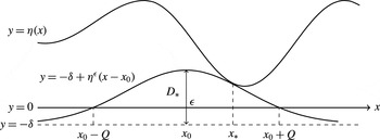
A sketch of the domain
 $D_{\ast }$
bounded by the curve
 $y=-\unicode[STIX]{x1D6FF}+\unicode[STIX]{x1D702}_{\unicode[STIX]{x1D716}}(x-x_{0})$
from above and by the
 $y$
-axis from below.

To prove the lower bound for
 $\check{\unicode[STIX]{x1D702}}$
we consider two cases. First, we assume that
 $\check{\unicode[STIX]{x1D702}}=0$
. Since
 $\unicode[STIX]{x1D702}$
does not vanish identically, for
 $d\in (0,d_{\ast })$
and
 $\unicode[STIX]{x1D6FF}>0$
there exists
 $\unicode[STIX]{x1D716}\in (\unicode[STIX]{x1D6FF},2\unicode[STIX]{x1D6FF})$
and
 $x_{0},x_{\ast }\in \mathbb{R}$
(see figure 6) such that
 $$\begin{eqnarray}\unicode[STIX]{x1D702}(x)\geqslant -\unicode[STIX]{x1D6FF}+\unicode[STIX]{x1D702}_{\unicode[STIX]{x1D716}}(x-x_{0})\quad \text{and}\quad \unicode[STIX]{x1D702}(x_{\ast })=-\unicode[STIX]{x1D6FF}+\unicode[STIX]{x1D702}_{\unicode[STIX]{x1D716}}(x_{\ast }-x_{0})>0.\end{eqnarray}$$
Let us apply the maximum principle to the superharmonic function
 $$\begin{eqnarray}U(x,y)=\unicode[STIX]{x1D713}_{d,\unicode[STIX]{x1D716}}(x-x_{0},y+d+\unicode[STIX]{x1D6FF})-\unicode[STIX]{x1D713}(x,y)\end{eqnarray}$$
in the domain
 $D_{\ast }=\{(x,y):~-Q<x-x_{0}<Q,~0<y<-\unicode[STIX]{x1D6FF}+\unicode[STIX]{x1D702}_{\unicode[STIX]{x1D716}}(x-x_{0})\}$
, where
 $Q>0$
is such that
 $\unicode[STIX]{x1D702}_{\unicode[STIX]{x1D716}}(Q)=\unicode[STIX]{x1D6FF}$
. Since
 $U$
is positive in
 $D_{\ast }$
and
 $U(x_{\ast },-\unicode[STIX]{x1D6FF}+\unicode[STIX]{x1D702}_{\unicode[STIX]{x1D716}}(x_{\ast }-x_{0}))$
vanishes, we obtain that
 $\unicode[STIX]{x2202}_{n}U(x_{\ast },-\unicode[STIX]{x1D6FF}+\unicode[STIX]{x1D702}_{\unicode[STIX]{x1D716}}(x_{\ast }-x_{0}))<0$
, and so
 $u_{d}^{\prime }(d)\leqslant \sqrt{3r}+O(\unicode[STIX]{x1D6FF})$
. Letting
 $\unicode[STIX]{x1D6FF}\rightarrow 0$
in this inequality, we arrive at
 $u_{d}^{\prime }(d)\leqslant \sqrt{3r}$
, which is impossible when
 $d$
is sufficiently small. The obtained contradiction shows that
 $\check{\unicode[STIX]{x1D702}}>0$
.
Now we assume that
 $\check{\unicode[STIX]{x1D702}}>0$
is less than
 $(2\unicode[STIX]{x1D714}_{0})^{-1/2}$
, because otherwise the required inequality is obviously true. To keep the same notation as above we put
 $d=\check{\unicode[STIX]{x1D702}}$
. Then for every
 $\unicode[STIX]{x1D6FF}\in (0,d)$
there exists
 $\unicode[STIX]{x1D716}\in (\unicode[STIX]{x1D6FF},2\unicode[STIX]{x1D6FF})$
and
 $x_{0},x_{\ast }\in \mathbb{R}$
such that
 $$\begin{eqnarray}\unicode[STIX]{x1D702}(x)\geqslant d-\unicode[STIX]{x1D6FF}+\unicode[STIX]{x1D702}_{\unicode[STIX]{x1D716}}(x-x_{0})\quad \text{and}\quad \unicode[STIX]{x1D702}(x_{\ast })=d-\unicode[STIX]{x1D6FF}+\unicode[STIX]{x1D702}_{\unicode[STIX]{x1D716}}(x_{\ast }-x_{0}).\end{eqnarray}$$
Applying the maximum principle to the superharmonic function
 $$\begin{eqnarray}U(x,y)=\unicode[STIX]{x1D713}_{d,\unicode[STIX]{x1D716}}(x-x_{0},y+\unicode[STIX]{x1D6FF})-\unicode[STIX]{x1D713}(x,y)\end{eqnarray}$$
in the domain
 $\{(x,y):~-\infty <x<+\infty ,~0<y<d-\unicode[STIX]{x1D6FF}+\unicode[STIX]{x1D702}_{\unicode[STIX]{x1D716}}(x-x_{0})\}$
, we conclude (in the same way as above) that
 $\unicode[STIX]{x2202}_{n}U(x_{\ast },d-\unicode[STIX]{x1D6FF}+\unicode[STIX]{x1D702}_{\unicode[STIX]{x1D716}}(x_{\ast }-x_{0}))<0$
. Therefore,
 $$\begin{eqnarray}u_{d}^{\prime }(d)=\check{\unicode[STIX]{x1D702}}^{-1}-\unicode[STIX]{x1D714}_{0}\check{\unicode[STIX]{x1D702}}/2\leqslant \sqrt{3r-\check{\unicode[STIX]{x1D702}}},\end{eqnarray}$$
which implies that
 $\check{\unicode[STIX]{x1D702}}^{-2}\leqslant 3r+\unicode[STIX]{x1D714}_{0}$
, and so
 $\check{\unicode[STIX]{x1D702}}\geqslant \min \{(6r)^{-1/2},(2\unicode[STIX]{x1D714}_{0})^{-1/2}\}$
. It should be noted that this inequality for
 $\check{\unicode[STIX]{x1D702}}$
also holds when
 $\check{\unicode[STIX]{x1D702}}\geqslant d_{0}$
, which completes the proof.☐
4.1 Uniform bound for the velocity field
To give a uniform bound for
 $\unicode[STIX]{x1D735}\unicode[STIX]{x1D713}$
, the main difficulty is the nonlinear term in (1.1), which does not allow us to apply the standard maximum principle for elliptic equations. This difficulty is circumvented in the next assertion.
Proposition 2. For every
 $R>r_{c}$
there exists
 $C(\unicode[STIX]{x1D714}_{0},R)$
(this constant does not depend on other parameters) such that if
 $(\unicode[STIX]{x1D713},\unicode[STIX]{x1D702})$
solves problem
 $P_{r}^{M}$
with
 $r\in (r_{c},R]$
, then the inequality
 $|\unicode[STIX]{x1D735}\unicode[STIX]{x1D713}(x,y)|\leqslant C(\unicode[STIX]{x1D714}_{0},R)$
holds for all
 $(x,y)\in \bar{D}$
.
Proof. Let
 $D_{t}=\{(x,y):~t\leqslant x\leqslant t+1,~0\leqslant y\leqslant \unicode[STIX]{x1D702}(x)\}$
for
 $t\in \mathbb{R}$
; our first aim is to show that
 $$\begin{eqnarray}\sup _{t\in \mathbb{R}}\int _{D_{t}}|\unicode[STIX]{x1D735}\unicode[STIX]{x1D713}|^{2}\,\text{d}x\,\text{d}y\leqslant C(\unicode[STIX]{x1D714}_{0},M,r),\end{eqnarray}$$
where the constant
 $C(\unicode[STIX]{x1D714}_{0},M,r)$
does not depend on other parameters.
Multiplying (1.1) by
 $\unicode[STIX]{x1D713}$
and integrating the result over
 $D_{t}$
, we apply the first Green’s formula, thus obtaining
 $$\begin{eqnarray}\displaystyle \int _{D_{t}}|\unicode[STIX]{x1D735}\unicode[STIX]{x1D713}|^{2}\,\text{d}x\,\text{d}y & = & \displaystyle \int _{D_{t}}\unicode[STIX]{x1D714}(\unicode[STIX]{x1D713})\unicode[STIX]{x1D713}\,\text{d}x\,\text{d}y+\int _{t}^{t+1}\unicode[STIX]{x1D735}\unicode[STIX]{x1D713}\cdot (-\unicode[STIX]{x1D702}^{\prime }(x),1)\,\text{d}x\nonumber\\ \displaystyle & & \displaystyle +\int _{0}^{\unicode[STIX]{x1D702}(t+1)}\unicode[STIX]{x1D713}_{x}(t+1,y)\unicode[STIX]{x1D713}(t+1,y)\,\text{d}y-\int _{0}^{\unicode[STIX]{x1D702}(t)}\unicode[STIX]{x1D713}_{x}(t,y)\unicode[STIX]{x1D713}(t,y)\,\text{d}y.\nonumber\\ \displaystyle & & \displaystyle\end{eqnarray}$$
Let us consider each of the four integrals on the right-hand side, denoted, say,
 $I_{1},~I_{2},~I_{3}$
and
 $I_{4}$
.
According to (1.5) the range of
 $\unicode[STIX]{x1D713}$
is
 $[0,1]$
, and so the definition of
 $\unicode[STIX]{x1D714}_{0}$
implies that
 $|I_{1}|\leqslant 3r\unicode[STIX]{x1D714}_{0}/2$
for all
 $t\in \mathbb{R}$
because
 $\unicode[STIX]{x1D702}(x)\leqslant 3r/2$
for all
 $x\in \mathbb{R}$
. Furthermore, the boundary condition (1.3) yields that
 $$\begin{eqnarray}\unicode[STIX]{x1D713}_{x}(x,\unicode[STIX]{x1D702}(x))=-\unicode[STIX]{x1D702}^{\prime }(x)\unicode[STIX]{x1D713}_{y}(x,\unicode[STIX]{x1D702}(x)).\end{eqnarray}$$
Then the Bernoulli equation (1.4) gives
 $$\begin{eqnarray}0<I_{2}=\int _{t}^{t+1}\sqrt{[3r-2\unicode[STIX]{x1D702}(x)][1+\unicode[STIX]{x1D702}^{\prime 2}(x)]}\,\text{d}x\leqslant \sqrt{3r(1+M^{2})}\quad \text{for all}~t\in \mathbb{R}.\end{eqnarray}$$
Our estimates of
 $|I_{3}|$
and
 $|I_{4}|$
are based on the equality
 $$\begin{eqnarray}\int _{0}^{\unicode[STIX]{x1D702}(t)}\unicode[STIX]{x1D713}_{x}(t,y)\unicode[STIX]{x1D713}(t,y)\,\text{d}y=2^{-1}\frac{\text{d}}{\text{d}t}\left[\int _{0}^{\unicode[STIX]{x1D702}(t)}\unicode[STIX]{x1D713}^{2}(t,y)\,\text{d}y-\unicode[STIX]{x1D702}(t)\right],\end{eqnarray}$$
which allows us to estimate
 $$\begin{eqnarray}\left|\int _{\mathbb{R}}\text{e}^{-|t-\tilde{t}|}\,\text{d}\tilde{t}\int _{0}^{\unicode[STIX]{x1D702}(\tilde{t})}\unicode[STIX]{x1D713}_{x}(\tilde{t},y)\unicode[STIX]{x1D713}(\tilde{t},y)\,\text{d}y\,\right|\quad \text{for all}~t\in \mathbb{R}.\end{eqnarray}$$
Indeed, multiplying the right-hand side of the equality by the corresponding exponential and integrating over
 $\mathbb{R}$
, we get after integration by parts that the last integral is less than or equal to
 $3r$
.
Thus, it follows from (4.13) and the obtained inequalities that
 $$\begin{eqnarray}\int _{\mathbb{R}}\text{e}^{-|t-\tilde{t}|}\,\text{d}\tilde{t}\int _{D_{\tilde{t}}}|\unicode[STIX]{x1D735}\unicode[STIX]{x1D713}|^{2}\,\text{d}x\,\text{d}y\leqslant C(\unicode[STIX]{x1D714}_{0},M,r)\quad \text{for all }t\in \mathbb{R}.\end{eqnarray}$$
After changing the order of integration, this gives
 $$\begin{eqnarray}\int _{D}|\unicode[STIX]{x1D735}\unicode[STIX]{x1D713}|^{2}\text{e}^{-|x-t|}\,\text{d}x\,\text{d}y\leqslant C(\unicode[STIX]{x1D714}_{0},M,r)\quad \text{for all }t\in \mathbb{R},\end{eqnarray}$$
which, in turn, yields (4.12).
To complete the proof, we apply some local estimates. First, we note that interior estimates and estimates near the bottom require only equation (1.1) and the boundary condition (1.2). The Schauder interior estimates (see Gilbarg & Trudinger Reference Gilbarg and Trudinger2001, theorem 6.2) and inequality (4.12) imply that
 $|\unicode[STIX]{x1D735}\unicode[STIX]{x1D713}|$
is bounded pointwise by a constant
 $C(\unicode[STIX]{x1D714}_{1},\unicode[STIX]{x1D716})$
in the domain
 $D_{\unicode[STIX]{x1D716}}$
for all points of which the distance from
 $\unicode[STIX]{x2202}D$
is not less than
 $\unicode[STIX]{x1D716}=\check{\unicode[STIX]{x1D702}}/3$
. Besides, combining local estimates near a smooth boundary (see Gilbarg & Trudinger Reference Gilbarg and Trudinger2001, corollary 8.36) and the inequality (4.12), one obtains that
 $|\unicode[STIX]{x1D735}\unicode[STIX]{x1D713}|$
is bounded pointwise by a constant
 $C(\unicode[STIX]{x1D714}_{0},\unicode[STIX]{x1D716})$
in the
 $\unicode[STIX]{x1D716}$
-neighbourhood of the bottom
 $\{x\in \mathbb{R},y=0\}$
. According to lemma 1,
 $\unicode[STIX]{x1D716}=\check{\unicode[STIX]{x1D702}}/3$
is greater than a positive constant depending only on
 $\unicode[STIX]{x1D714}_{0}$
and
 $R$
. Thus, it remains to estimate
 $\unicode[STIX]{x1D735}\unicode[STIX]{x1D713}$
near the free surface.
For this purpose we use theorem 8.25 in Gilbarg & Trudinger (Reference Gilbarg and Trudinger2001) for solutions of the equation
 $\unicode[STIX]{x1D6FB}^{2}\unicode[STIX]{x1D713}^{\ast }+\unicode[STIX]{x1D714}^{\prime }(\unicode[STIX]{x1D713})\unicode[STIX]{x1D713}^{\ast }=0$
, thus obtaining
 $$\begin{eqnarray}\sup _{B_{a}(Z_{0})}\unicode[STIX]{x1D713}_{m}^{\ast }\leqslant C(\unicode[STIX]{x1D714}_{1})a^{-1}\Vert \unicode[STIX]{x1D713}_{m}^{\ast }\Vert _{L^{2}(B_{2a}(Z_{0}))}.\end{eqnarray}$$
Here
 $\unicode[STIX]{x1D713}^{\ast }$
stands for either of the first derivatives of
 $\unicode[STIX]{x1D713}$
,
 $a>0$
is fixed and
 $Z_{0}$
is an arbitrary point of
 $D$
; by
 $B_{a}(Z_{0})$
we denote the open circle of radius
 $a$
centred at
 $Z_{0}$
and
 $$\begin{eqnarray}\unicode[STIX]{x1D713}_{m}^{\ast }(x,y)=\left\{\begin{array}{@{}ll@{}}\max \{\unicode[STIX]{x1D713}^{\ast }(x,y),m\}\quad & \text{when }(x,y)\in D,\\ m\quad & \text{when }(x,y)\notin D,\end{array}\right.\end{eqnarray}$$
where
 $m=\sup _{\unicode[STIX]{x2202}D\cap B_{2a}(Z_{0})}\unicode[STIX]{x1D713}^{\ast }$
.
From the Bernoulli equation (1.4) we see that
 $m\leqslant \sqrt{3r}$
in inequality (4.20) with
 $B_{a}(Z_{0})$
having
 $a=\unicode[STIX]{x1D716}=\check{\unicode[STIX]{x1D702}}/3$
and centred arbitrarily on the free surface. Then combining (4.12) and (4.20), we find that
 $\unicode[STIX]{x1D713}^{\ast }$
is bounded from above by
 $C(\unicode[STIX]{x1D714}_{1},M,r)$
in the
 $\unicode[STIX]{x1D716}$
-neighbourhood of the free surface. Since the same argument is valid for
 $-\unicode[STIX]{x1D713}^{\ast }$
, we obtain that
 $$\begin{eqnarray}|\unicode[STIX]{x1D735}\unicode[STIX]{x1D713}(x,y)|\leqslant C(\unicode[STIX]{x1D714}_{1},M,r)\quad \text{for all }(x,y)\in D.\end{eqnarray}$$
In order to exclude the dependence of the right-hand side constant on the parameter
 $M$
, let us consider the following function:
 $$\begin{eqnarray}T(x,y)=-3r+|\unicode[STIX]{x1D735}\unicode[STIX]{x1D713}|^{2}+2y+2\unicode[STIX]{x1D6FA}(\unicode[STIX]{x1D713}).\end{eqnarray}$$
A direct calculation gives that
 $\unicode[STIX]{x1D6FB}^{2}T\geqslant -2\unicode[STIX]{x1D714}_{0}^{2}$
in
 $D$
, and so
 $T^{\ast }=T+\unicode[STIX]{x1D714}_{0}^{2}y^{2}$
is a subharmonic function in
 $D$
. Since
 $T^{\ast }$
is bounded, we apply the maximum principle in the form due to Cabre (Reference Cabre1995) (see theorem 1.4 in his paper). It gives that the supremum of
 $T^{\ast }$
is attained either on the free surface, where
 $T^{\ast }$
is bounded by
 $2\unicode[STIX]{x1D714}_{0}+9/4\unicode[STIX]{x1D714}_{0}^{2}r^{2}$
, or on the bottom. The latter is not possible, since
 $T_{y}^{\ast }=2$
on the bottom. Therefore,
 $T^{\ast }\leqslant C(\unicode[STIX]{x1D714}_{0},R)$
throughout
 $D$
, which proves the proposition provided the definition of
 $T$
is taken into account. It should be noted that a version of this calculation was used by Constantin & Strauss (Reference Constantin and Strauss2004); see lemma 7.2 of their paper.☐
4.2 Bounds for solutions of
$P_{r}^{M}$
in the near-critical case

The slope of
 $\unicode[STIX]{x1D702}$
is bounded by the definition of problem
 $P_{r}^{M}$
. However, this restriction does not prevent the presence of stagnation points on
 $\unicode[STIX]{x1D702}$
. Nevertheless, if
 $r$
is sufficiently close to its critical value
 $r_{c}$
, then every solution of
 $P_{r}^{M}$
is of small amplitude, and so there are no stagnation points on
 $\unicode[STIX]{x1D702}$
. The following assertion makes both these properties rigorous.
Theorem 4. Let
 $M$
be positive. If
 $r$
is subject to condition (2.10), then the following assertions are true.
-
(1) For every
$\unicode[STIX]{x1D716}>0$
there exists a constant
$r^{\prime }(\unicode[STIX]{x1D716},M,\unicode[STIX]{x1D714}_{0})>r_{c}$
such that (4.24)where
$$\begin{eqnarray}\sup _{x\in \mathbb{R}}|\unicode[STIX]{x1D702}(x)-d_{+}(r)|<\unicode[STIX]{x1D716},\end{eqnarray}$$
$d_{+}(r)$
is defined in § 2.1 and
$\unicode[STIX]{x1D702}$
is the second component of a solution to problem
$P_{r}^{M}$
with
$r\in (r_{c},r^{\prime }]$
.
-
(2) There exist
$r^{\prime \prime }(M,\unicode[STIX]{x1D714}_{1})>r_{c}$
and
$\unicode[STIX]{x1D6FF}(M,\unicode[STIX]{x1D714}_{1})>0$
such that
$\unicode[STIX]{x1D713}_{y}>\unicode[STIX]{x1D6FF}(M,\unicode[STIX]{x1D714}_{1})$
in
$D$
, where
$\unicode[STIX]{x1D713}$
is the first component of a solution of problem
$P_{r}^{M}$
with
$r\in (r_{c},r^{\prime \prime }]$
.




Proof. To prove (1) we put
 $w(q,p)=h(q,p)-H(p)$
, where
 $h$
is a solution of problem (3.2)–(3.4) in
 $S=\{(q,p):q\in \mathbb{R},p\in (0,1)\}$
and
 $H$
is defined by formula (3.6). It is convenient to introduce
 $w$
because
 $\unicode[STIX]{x1D702}(x)=h(x,1)$
,
 $x\in \mathbb{R}$
and
 $d_{+}(r)=H(1,\unicode[STIX]{x1D706}_{+}(r))$
. Relations (3.5) between the derivatives of
 $\unicode[STIX]{x1D713}$
and
 $h$
yield that
 $h$
,
 $h_{p}^{-1}$
and
 $f=h_{q}h_{p}^{-1}$
are bounded by a constant depending on
 $\unicode[STIX]{x1D714}_{0}$
and
 $R$
(see proposition 2).
Let
 $\unicode[STIX]{x1D719}_{0}$
be the eigenfunction of the spectral problem (3.7)–(3.9) corresponding to
 $\unicode[STIX]{x1D707}_{0}$
. According to assertion (i) of proposition 1,
 $\unicode[STIX]{x1D707}_{0}$
is negative when
 $H=H(p,\unicode[STIX]{x1D706}_{+}(r))$
. Putting
 $$\begin{eqnarray}w_{0}(q)=\int _{0}^{1}w(q,p)\unicode[STIX]{x1D719}_{0}(p)H_{p}^{-1}(p)\,\text{d}p\quad \text{and}\quad f_{0}(q)=\int _{0}^{1}f(q,p)\unicode[STIX]{x1D719}_{0}(p)\,\text{d}p,\end{eqnarray}$$
we obtain from problems (3.2)–(3.4) the equality
 $$\begin{eqnarray}\int _{0}^{1}\left[\frac{H_{p}^{3}f^{2}}{2}+\frac{(2h_{p}+H_{p})w_{p}^{2}}{2h_{p}^{2}}\right]\frac{\unicode[STIX]{x1D719}_{0}^{\prime }}{H_{p}^{3}}\,\text{d}p=\unicode[STIX]{x1D707}_{0}w_{0}-f_{0}^{\prime }.\end{eqnarray}$$
It is analogous to equality (2.11) in Kozlov et al. (Reference Kozlov, Kuznetsov and Lokharu2015), whose derivation is implicitly given by Wheeler (Reference Wheeler2015) in the proof of his lemma 3.1.
Multiplying (4.26) by
 $\text{e}^{-\unicode[STIX]{x1D717}|q-q_{0}|}$
with some
 $\unicode[STIX]{x1D717}>0$
and
 $q_{0}\in \mathbb{R}$
, and integrating the result over
 $\mathbb{R}$
, we estimate both integrals on the right-hand side, thus obtaining
 $$\begin{eqnarray}\displaystyle & & \displaystyle \int _{S}\left[\frac{H_{p}^{3}f^{2}}{2}+\frac{(2h_{p}+H_{p})w_{p}^{2}}{2h_{p}^{2}}\right]\frac{\unicode[STIX]{x1D719}_{0}^{\prime }}{H_{p}^{3}}\text{e}^{-\unicode[STIX]{x1D717}|q-q_{0}|}\,\text{d}q\,\text{d}p\nonumber\\ \displaystyle & & \displaystyle \qquad \leqslant |\unicode[STIX]{x1D707}_{0}|\int _{-\infty }^{+\infty }|w_{0}|\,\text{e}^{-\unicode[STIX]{x1D717}|q-q_{0}|}\,\text{d}q+C_{4}(\unicode[STIX]{x1D714}_{0})\unicode[STIX]{x1D717}\int _{S}|\,f|\,\text{e}^{-\unicode[STIX]{x1D717}|q-q_{0}|}\,\text{d}q.\end{eqnarray}$$
Here
 $C_{4}$
is the same constant as in proposition 1, and it arises after integration by parts in the second integral. Since
 $w_{0}$
and
 $f$
are bounded on
 $\bar{S}$
, both integrals on the right-hand side are convergent. Therefore, the first term is bounded by
 $C(\unicode[STIX]{x1D714}_{0})|\unicode[STIX]{x1D707}_{0}|/\unicode[STIX]{x1D717}$
, whereas the second one is less than or equal to
 $$\begin{eqnarray}C(\unicode[STIX]{x1D714}_{0})\sqrt{\unicode[STIX]{x1D717}}\left[\int _{S}f^{2}\text{e}^{-\unicode[STIX]{x1D717}|q-q_{0}|}\,\text{d}q\,\text{d}p\right]^{1/2},\end{eqnarray}$$
which is a consequence of the Schwarz inequality. Putting
 $\unicode[STIX]{x1D717}=\sqrt{|\unicode[STIX]{x1D707}_{0}|}$
, we see that (4.27) implies the following inequality:
 $$\begin{eqnarray}I^{2}-C(\unicode[STIX]{x1D714}_{0})|\unicode[STIX]{x1D707}_{0}|^{1/4}I-C(\unicode[STIX]{x1D714}_{0})\sqrt{|\unicode[STIX]{x1D707}_{0}|}\leqslant 0,\quad \text{where }I=\left[\int _{S}f^{2}\text{e}^{-\unicode[STIX]{x1D703}|q-q_{0}|}\right]^{1/2}\!.\end{eqnarray}$$
Here, it is also taken into account that
 $\min _{p\in [0,1]}\unicode[STIX]{x1D719}^{\prime }(p)\geqslant C$
(see assertion (iii) of proposition 1), and the last positive constant depends only on
 $\unicode[STIX]{x1D714}_{0}$
. Then the inequality for
 $I$
gives that
 $I\leqslant C(\unicode[STIX]{x1D714}_{0})|\unicode[STIX]{x1D707}_{0}|^{1/4}$
. Combining this and (4.27), we arrive at the inequality
 $$\begin{eqnarray}\int _{S}\left[\frac{H_{p}^{3}f^{2}}{2}+\frac{(2h_{p}+H_{p})w_{p}^{2}}{2h_{p}^{2}}\right]\frac{\unicode[STIX]{x1D719}_{0}^{\prime }}{H_{p}^{3}}\text{e}^{-\unicode[STIX]{x1D703}|q-q_{0}|}\,\text{d}q\,\text{d}p\leqslant C(\unicode[STIX]{x1D714}_{0})\sqrt{|\unicode[STIX]{x1D707}_{0}|}.\end{eqnarray}$$
Furthermore, by virtue of the Schwarz inequality, we have that
 $$\begin{eqnarray}\int _{q_{0}-1}^{q_{0}+1}\!\int _{0}^{1}|w_{p}|\,\text{d}p\,\text{d}q\leqslant \left[\int _{q_{0}-1}^{q_{0}+1}\!\int _{0}^{1}\frac{|w_{p}|^{2}}{h_{p}}\,\text{d}p\,\text{d}q\right]^{1/2}\left[\int _{q_{0}-1}^{q_{0}+1}\!\int _{0}^{1}h_{p}\,\text{d}p\,\text{d}q\right]^{1/2},\end{eqnarray}$$
and the last expression is bounded by
 $C(\unicode[STIX]{x1D714}_{0})|\unicode[STIX]{x1D707}_{0}|^{1/4}$
in view of (4.30). This fact and the inequality
 $|w(q,1)|\leqslant \int _{0}^{1}|w_{p}(q,p)|\,\text{d}p$
give us that
 $$\begin{eqnarray}\int _{q_{0}-1}^{q_{0}+1}|\unicode[STIX]{x1D702}(q)-d_{+}(r)|\,\text{d}q\leqslant C(\unicode[STIX]{x1D714}_{0})|\unicode[STIX]{x1D707}_{0}|^{1/4}\quad \text{for all}~q_{0}\in \mathbb{R},\end{eqnarray}$$
because
 $w(q,1)=\unicode[STIX]{x1D702}(q)-d_{+}(r)$
.
According to assertion (i) of proposition 1, we have that
 $\unicode[STIX]{x1D707}_{0}(\unicode[STIX]{x1D706})\rightarrow 0$
as
 $\unicode[STIX]{x1D706}\rightarrow \unicode[STIX]{x1D706}_{c}$
, and so the last inequality implies that for every
 $\unicode[STIX]{x1D716}>0$
there exists
 $r^{\prime }=r^{\prime }(\unicode[STIX]{x1D716},M,\unicode[STIX]{x1D714}_{0})$
such that
 $|\unicode[STIX]{x1D702}(q)-d_{+}(r)|<\unicode[STIX]{x1D716}$
for all
 $q\in \mathbb{R}$
and all
 $r\in (r_{c},r^{\prime })$
. Indeed,
 $|\unicode[STIX]{x1D702}^{\prime }(q)|\leqslant M$
almost everywhere on
 $\mathbb{R}$
being the second component of a solution of problem
 $P_{r}^{M}$
.
Now we turn to assertion (2) for the first component of a solution to problem
 $P_{r}^{M}$
. First, we show that
 $\unicode[STIX]{x1D713}_{y}$
is separated from zero on
 $\unicode[STIX]{x2202}D$
when
 $r$
is close to
 $r_{c}$
.
Since the boundary conditions (1.3) and (1.4) imply that
 $$\begin{eqnarray}\{1+[\unicode[STIX]{x1D702}^{\prime }(x)]^{2}\}\unicode[STIX]{x1D713}_{y}^{2}(x,\unicode[STIX]{x1D702}(x))=3r-2\unicode[STIX]{x1D702}(x)\quad \text{for all}~x\in \mathbb{R},\end{eqnarray}$$
the inequality
 $[\unicode[STIX]{x1D713}_{y}(x,\unicode[STIX]{x1D702}(x))]^{2}\geqslant [3r-2\unicode[STIX]{x1D702}(x)]/(1+M^{2})$
holds for all
 $~x\in \mathbb{R}$
. Let us show that the expression on the right-hand side is separated from zero by a positive constant depending only on
 $\unicode[STIX]{x1D714}_{0}$
. For this purpose we write
 $$\begin{eqnarray}3r-2\unicode[STIX]{x1D702}=3r-2d_{+}(r)-2[\unicode[STIX]{x1D702}-d_{+}(r)]=[\unicode[STIX]{x1D706}_{+}(r)]^{2}-2\unicode[STIX]{x1D6FA}(1)-2[\unicode[STIX]{x1D702}-d_{+}(r)],\end{eqnarray}$$
where the last equality is a consequence of (2.4). In view of (2.10) we have
 $$\begin{eqnarray}[\unicode[STIX]{x1D706}_{+}(r)]^{2}-2\unicode[STIX]{x1D6FA}(1)=\unicode[STIX]{x1D706}_{0}^{2}-2\unicode[STIX]{x1D6FA}(1)+[\unicode[STIX]{x1D706}_{+}(r)]^{2}-\unicode[STIX]{x1D706}_{0}^{2}\geqslant (\unicode[STIX]{x1D706}_{c}-\unicode[STIX]{x1D706}_{0})\unicode[STIX]{x1D706}_{c}/4,\end{eqnarray}$$
but assertion (1) of theorem 4 with
 $\unicode[STIX]{x1D716}=(\unicode[STIX]{x1D706}_{c}-\unicode[STIX]{x1D706}_{0})\unicode[STIX]{x1D706}_{c}/16$
yields that there exists
 $r^{\prime }(M,\unicode[STIX]{x1D714}_{0})$
such that
 $$\begin{eqnarray}2|\unicode[STIX]{x1D702}-d_{+}(r)|\leqslant (\unicode[STIX]{x1D706}_{c}-\unicode[STIX]{x1D706}_{0})\unicode[STIX]{x1D706}_{c}/8\quad \text{for all}~r\in (r_{c},r^{\prime }].\end{eqnarray}$$
Therefore,
 $$\begin{eqnarray}[\unicode[STIX]{x1D713}_{y}(x,\unicode[STIX]{x1D702}(x))]^{2}\geqslant (\unicode[STIX]{x1D706}_{c}-\unicode[STIX]{x1D706}_{0})\unicode[STIX]{x1D706}_{c}/[8(1+M^{2})]\quad \text{for all}~x\in \mathbb{R}.\end{eqnarray}$$
To estimate
 $\unicode[STIX]{x1D713}_{y}$
near the bottom we use the problem (3.2)–(3.4) because the maximum principle (see Cabre Reference Cabre1995, theorem 1.4) is applicable to it. We choose
 $\unicode[STIX]{x1D706}_{\ast }$
so that
 $\sup _{x\in \mathbb{R}}\unicode[STIX]{x1D702}(x)=H(p,\unicode[STIX]{x1D706}_{\ast })$
, and put
 $w(q,p)=h(q,p)-H(p,\unicode[STIX]{x1D706}_{\ast })$
. Since
 $w(q,0)=0$
for all
 $q\in \mathbb{R}$
and
 $w(q,1)<0$
, the maximum principle implies that
 $w<0$
in
 $S$
and
 $w_{p}(q,0)<0$
. In other words,
 $h_{p}(q,0)<H_{p}(0,\unicode[STIX]{x1D706}_{\ast })$
, and so
 $$\begin{eqnarray}\unicode[STIX]{x1D713}_{y}(x,0)\geqslant [H_{p}(0,\unicode[STIX]{x1D706}_{\ast })]^{-1}\geqslant [H_{p}(0,\unicode[STIX]{x1D706}_{+}(r))]^{-1}\geqslant \sqrt{(\unicode[STIX]{x1D706}_{c}-\unicode[STIX]{x1D706}_{0})\unicode[STIX]{x1D706}_{c}/4}.\end{eqnarray}$$
Here the second inequality is a consequence of (3.5).
The obtained estimates of
 $\unicode[STIX]{x1D713}_{y}$
on
 $\unicode[STIX]{x2202}D$
allow us to apply theorem 8.26 from the book by Gilbarg & Trudinger (Reference Gilbarg and Trudinger2001) to the equation
 $\unicode[STIX]{x1D6FB}^{2}\unicode[STIX]{x1D713}_{y}+\unicode[STIX]{x1D714}^{\prime }(\unicode[STIX]{x1D713})\unicode[STIX]{x1D713}_{y}=0$
, thus demonstrating that
 $\unicode[STIX]{x1D713}_{y}$
is separated from zero in a neighbourhood of
 $\unicode[STIX]{x2202}D$
. According to this theorem we have
 $$\begin{eqnarray}\Vert \unicode[STIX]{x1D713}_{y}^{-}\Vert _{L^{2}(B_{6a}(Z))}\leqslant C(\unicode[STIX]{x1D714}_{1})\inf _{B_{3a}(Z)}\unicode[STIX]{x1D713}_{y}^{-},\end{eqnarray}$$
where
 $Z$
is an arbitrary point of
 $\unicode[STIX]{x2202}D$
,
 $$\begin{eqnarray}\unicode[STIX]{x1D713}_{y}^{-}(x,y)=\left\{\begin{array}{@{}ll@{}}\min \{\unicode[STIX]{x1D713}_{y},m\}\quad & \text{when }(x,y)\in D,\\ m\quad & \text{when }(x,y)\notin D,\end{array}\right.\end{eqnarray}$$
and
 $m=\inf _{B_{12a}(Z)\cap \unicode[STIX]{x2202}D}\unicode[STIX]{x1D713}_{y}$
. We recall that
 $B_{a}(Z)$
denotes the open circle of radius
 $a$
centred at
 $Z$
.
It is essential that the constant in (4.39) depends only on
 $\unicode[STIX]{x1D714}_{1}$
and is independent of
 $a$
. Indeed, lemma 1 and inequality (2.10) imply that
 $$\begin{eqnarray}C_{1}(\unicode[STIX]{x1D714}_{0})<3a<C_{2}(\unicode[STIX]{x1D714}_{0}),\end{eqnarray}$$
where both constants are positive and depend only on
 $\unicode[STIX]{x1D714}_{0}$
. Since the free surface is a Lipschitz curve with the constant
 $\sqrt{1+M^{2}}$
, a large part of the ball
 $B_{6a}(Z)$
belongs to the complement of
 $D$
for every
 $Z\in \unicode[STIX]{x2202}D$
(this is obvious for the flat bottom), and so
 $\Vert \unicode[STIX]{x1D713}_{y}^{-}\Vert _{L^{2}(B_{6a}(Z))}\geqslant C(M)\,m$
. Combining this inequality and (4.39), we get that
 $$\begin{eqnarray}\inf _{B_{3a}(Z)\cap D}\unicode[STIX]{x1D713}_{y}\geqslant C(M,\unicode[STIX]{x1D714}_{1})m\quad \text{for every }Z\in \unicode[STIX]{x2202}D.\end{eqnarray}$$
The expression on the right-hand side is greater than some positive constant
 $C_{1}(M,\unicode[STIX]{x1D714}_{1})$
, and so the required inequality holds in the whole domain
 $D$
because it is covered by circles
 $B_{3a}(Z)$
with
 $Z\in \unicode[STIX]{x2202}D$
. This completes the proof.☐
Now, we turn to estimating Hölder norms for derivatives of solutions to problem
 $P_{r}^{M}$
. The corresponding bound will be obtained under the assumption that the horizontal component of the velocity field is uniformly separated from zero in
 $\bar{D}$
.
Proposition 3. Let
 $(\unicode[STIX]{x1D713},\unicode[STIX]{x1D702})$
be a solution of problem
 $P_{r}^{M}$
with
 $M>0$
and
 $r\in (r_{c},R]$
, where
 $R\in (r_{c},r_{0})$
. If
 $\unicode[STIX]{x1D713}_{y}>\unicode[STIX]{x1D6FF}$
in
 $\bar{D}$
for some
 $\unicode[STIX]{x1D6FF}>0$
, then there exist
 $\unicode[STIX]{x1D6FC}\in (0,1)$
and
 $C>0$
(both depend on
 $M$
,
 $R$
,
 $\unicode[STIX]{x1D6FF}$
and
 $\unicode[STIX]{x1D714}_{1}$
) such that the following inequalities hold:
 $$\begin{eqnarray}\Vert \unicode[STIX]{x1D713}\Vert _{C^{2,\unicode[STIX]{x1D6FC}}(\bar{D})}\leqslant C\quad \text{and}\quad \Vert \unicode[STIX]{x1D702}\Vert _{C^{2,\unicode[STIX]{x1D6FC}}(\mathbb{R})}\leqslant C.\end{eqnarray}$$
Proof. In view of assumptions imposed on
 $(\unicode[STIX]{x1D713},\unicode[STIX]{x1D702})$
, proposition 2 implies that
 $h$
– the corresponding solution of problem (3.2)–(3.4) – satisfies the inequalities
 $$\begin{eqnarray}0<C(\unicode[STIX]{x1D714}_{1},R)\leqslant h_{p}\leqslant \unicode[STIX]{x1D6FF}^{-1}\quad \text{in }\bar{S}=\mathbb{R}\times [0,1].\end{eqnarray}$$
Let us show that there exist
 $\unicode[STIX]{x1D6FC}>0$
and a positive constant
 $C^{\prime }(R,\unicode[STIX]{x1D714}_{1})$
such that the inequality
 $$\begin{eqnarray}\Vert h\Vert _{C^{1,\unicode[STIX]{x1D6FC}}(\bar{S})}\leqslant C^{\prime }(R,\unicode[STIX]{x1D714}_{1})\end{eqnarray}$$
holds. Since
 $\unicode[STIX]{x2202}S$
consists of two straight lines and the Dirichlet boundary condition is fulfilled when
 $p=0$
, the only difficulty is to prove the estimate near the line
 $\{q\in \mathbb{R},p=1\}$
(cf. Gilbarg & Trudinger Reference Gilbarg and Trudinger2001, theorems 13.1 and 13.2). To overcome this difficulty we use the local estimates of Ladyzhenskaya & Uraltseva (Reference Ladyzhenskaya and Uraltseva1964) (see the proof of theorem 2.1, chapter 10). For this purpose we write the quasilinear equation (3.2) in divergence form and complement it by the boundary condition (3.4) written in line with the form of the equation, namely,
 $$\begin{eqnarray}[a_{1}(h_{q},h_{p})]_{q}+[a_{2}(h_{q},h_{p})]_{p}-\unicode[STIX]{x1D714}=0,\quad [a_{2}(h_{q},h_{p})+\unicode[STIX]{x1D719}(h)]_{p=1}=0,\end{eqnarray}$$
where
 $$\begin{eqnarray}a_{1}(h_{q},h_{p})=\frac{h_{q}}{h_{p}},\quad a_{2}(h_{q},h_{p})=-\frac{1+h_{q}^{2}}{2h_{p}^{2}}\quad \text{and}\quad \unicode[STIX]{x1D719}(h)=2h-3r.\end{eqnarray}$$
All conditions required in the mentioned theorem are fulfilled for
 $a_{1}$
,
 $a_{2}$
and
 $\unicode[STIX]{x1D719}$
because of the two-sided restriction (4.44) which, in turn, yields (4.45).
The next step is to apply results of Agmon, Douglis & Nirenberg (Reference Agmon, Douglis and Nirenberg1959) to problem (4.46)–(4.47). In particular, their theorem 11.2 yields that
 $h\in C^{2,\unicode[STIX]{x1D6FC}}(\bar{S})$
but does not provide a bound for
 $\Vert h\Vert _{C^{2,\unicode[STIX]{x1D6FC}}(\bar{S})}$
. For this purpose we rewrite this problem as follows:
 $$\begin{eqnarray}\left.\begin{array}{@{}c@{}}\displaystyle h_{qq}-2h_{q}h_{p}^{-1}h_{qp}+(1+h_{q}^{2})h_{p}^{-2}h_{pp}+\unicode[STIX]{x1D714}(p)h_{p}=0\text{ in }S,\\ \displaystyle (1+h_{q}^{2})h_{p}^{-2}-(3r-2h)=0~\text{when }p=1,\quad h=0~\text{when }p=0.\end{array}\right\}\end{eqnarray}$$
Now we are in a position to use another result of Ladyzhenskaya & Uraltseva (Reference Ladyzhenskaya and Uraltseva1964); their theorem 3.1, chapter 10, shows that there exists a bound for
 $\Vert h\Vert _{C^{2,\unicode[STIX]{x1D6FC}}(\bar{S})}$
depending only on
 $M$
,
 $R$
,
 $\unicode[STIX]{x1D6FF}$
and
 $\unicode[STIX]{x1D714}_{1}$
. Thus, both estimates (4.43) are true in view of formulae (3.5) and inequalities (4.44).☐
5 Proof of theorem 2
Let us prove the following assertion that is slightly stronger than theorem 2.
Theorem 5. There exist
 $r^{\prime \prime }\in (r_{c},r_{0})$
and positive
 $C$
and
 $\unicode[STIX]{x1D703}$
(
 $r^{\prime \prime }$
depends on
 $M$
and
 $\unicode[STIX]{x1D714}_{1}$
, whereas
 $C$
and
 $\unicode[STIX]{x1D703}$
depend only on
 $\unicode[STIX]{x1D714}_{0}$
) such that any two solutions
 $(\unicode[STIX]{x1D713}^{(1)},\unicode[STIX]{x1D702}^{(1)})$
and
 $(\unicode[STIX]{x1D713}^{(2)},\unicode[STIX]{x1D702}^{(2)})$
of problem
 $P_{r}^{M}$
with
 $r\in (r_{c},r^{\prime \prime }]$
satisfy the inequality
 $$\begin{eqnarray}\displaystyle & & \displaystyle \int _{S}|\unicode[STIX]{x1D735}h^{(1)}-\unicode[STIX]{x1D735}h^{(2)}|^{2}\,\text{e}^{-\unicode[STIX]{x1D703}|x-x_{0}|}\,\text{d}q\,\text{d}p\nonumber\\ \displaystyle & & \displaystyle \qquad \leqslant C[|\unicode[STIX]{x1D702}^{(1)}(q_{0})-\unicode[STIX]{x1D702}^{(2)}(q_{0})|^{2}+|\unicode[STIX]{x1D702}_{x}^{(1)}(q_{0})-\unicode[STIX]{x1D702}_{x}^{(2)}(q_{0})|^{2}].\end{eqnarray}$$
Here
 $q_{0}\in \mathbb{R}$
is arbitrary, whereas
 $h^{(1)}$
and
 $h^{(2)}$
correspond to
 $(\unicode[STIX]{x1D713}^{(1)},\unicode[STIX]{x1D702}^{(1)})$
and
 $(\unicode[STIX]{x1D713}^{(2)},\unicode[STIX]{x1D702}^{(2)})$
through the partial hodograph transform.
It is easy to see that theorem 2 is a consequence of theorem 5. Our proof of the latter theorem is based on another form of problem (3.2)–(3.4), namely, a system of equations proposed by Groves & Wahlén (Reference Groves and Wahlén2008) (see (5.2) and (5.3) below).
5.1 A system of first order equivalent to problem (3.2)–(3.4)
In order to write problem (3.2)–(3.4) as an equivalent system of first order, we introduce the second unknown
 $f=h_{q}/h_{p}$
complementing
 $h$
and obtain
 $$\begin{eqnarray}\displaystyle & \displaystyle h_{q}=fh_{p}, & \displaystyle\end{eqnarray}$$
 $$\begin{eqnarray}\displaystyle & \displaystyle f_{q}=-{\textstyle \frac{1}{2}}{\mathcal{A}}(f,h)+\unicode[STIX]{x1D714}(p). & \displaystyle\end{eqnarray}$$
Here
 $(q,p)\in S$
and
 ${\mathcal{A}}$
is a nonlinear operator which we define by virtue of the integral identity
 $$\begin{eqnarray}\int _{0}^{1}{\mathcal{A}}(f,h)\unicode[STIX]{x1D6F7}\,\text{d}p=\int _{0}^{1}(f^{2}+h_{p}^{-2})\unicode[STIX]{x1D6F7}_{p}\,\text{d}p-[\{3r-2h(q,p)\}\unicode[STIX]{x1D6F7}(p)]_{p=1}.\end{eqnarray}$$
It must hold for every
 $\unicode[STIX]{x1D6F7}\in H_{0}^{1}(0,1)$
; this space consists of continuous functions which vanish at
 $p=0$
and whose derivatives belong to
 $L^{2}(0,1)$
. The last identity is well defined because the functions
 $f$
and
 $h_{p}^{-1}$
are bounded when
 $(\unicode[STIX]{x1D713},\unicode[STIX]{x1D702})$
is a solution of problem
 $P_{r}^{M}$
(see proposition 2).
This weak formulation allows us to use the technique developed in Kozlov & Maz’ya (Reference Kozlov and Maz’ya1999) (see also Kozlov & Maz’ya Reference Kozlov and Maz’ya2004) for ordinary differential equations with operator coefficients. It is also worth mentioning that the explicit form of
 ${\mathcal{A}}$
(the differential expression and boundary operators) can be found in Groves & Wahlén (Reference Groves and Wahlén2008).
5.1.1 Linearisation near a stream solution
Let us linearise (5.2) and (5.3) near the stream solution
 $H(p,\unicode[STIX]{x1D706}_{+}(r))$
, for which purpose we put
 $h=H+w$
, and so the pair
 $(w,f)$
must satisfy the following system:
 $$\begin{eqnarray}\displaystyle & \displaystyle w_{q}-fH_{p}={\mathcal{N}}_{1}(w,f), & \displaystyle\end{eqnarray}$$
 $$\begin{eqnarray}\displaystyle & \displaystyle f_{q}-{\mathcal{L}}(w)={\mathcal{N}}_{2}(w,f). & \displaystyle\end{eqnarray}$$
Here
 $(q,p)\in S$
and
 ${\mathcal{N}}_{1}(w,f)=fw_{p}$
, whereas the operators
 ${\mathcal{L}}$
and
 ${\mathcal{N}}_{2}$
are defined in the same way as
 ${\mathcal{A}}$
. Their action on functions given on the cross-section of
 $S$
is described by the integral identities
 $$\begin{eqnarray}\displaystyle & \displaystyle \int _{0}^{1}{\mathcal{L}}(w)\unicode[STIX]{x1D6F7}\,\text{d}p=\int _{0}^{1}\frac{w_{p}\unicode[STIX]{x1D6F7}_{p}}{H_{p}^{3}}\,\text{d}p-[w\unicode[STIX]{x1D6F7}]_{p=1}, & \displaystyle\end{eqnarray}$$
 $$\begin{eqnarray}\displaystyle & \displaystyle \int _{0}^{1}{\mathcal{N}}_{2}(w,f)\unicode[STIX]{x1D6F7}\,\text{d}p=-\int _{0}^{1}\left[\frac{w_{p}^{3}}{H_{p}^{3}h_{p}^{2}}+\frac{3}{2}\frac{w_{p}^{2}}{H_{p}^{2}h_{p}^{2}}+\frac{f^{2}}{2}\right]\unicode[STIX]{x1D6F7}_{p}\,\text{d}p, & \displaystyle\end{eqnarray}$$
which must be fulfilled for every
 $\unicode[STIX]{x1D6F7}\in H_{0}^{1}(0,1)$
. It should be noted that the identity for
 ${\mathcal{L}}$
is nothing else than the weak representation of the spectral problem (3.7)–(3.9).
Using theorem 4 and proposition 3, we prove the following assertion.
Lemma 2. For every positive
 $\unicode[STIX]{x1D716}$
and
 $M$
there exists
 $r^{\ast }\in (r_{c},r_{0})$
(depending on
 $M,\unicode[STIX]{x1D716}$
and
 $\unicode[STIX]{x1D714}_{1}$
) such that if
 $(\unicode[STIX]{x1D713},\unicode[STIX]{x1D702})$
is a solution of problem
 $P_{r}^{M}$
with
 $r\in (r_{c},r^{\ast }]$
, then the inequality
 $$\begin{eqnarray}\Vert w\Vert _{C^{2}(\bar{S})}+\Vert \,f\Vert _{C^{1}(\bar{S})}<\unicode[STIX]{x1D716}\end{eqnarray}$$
holds for the pair
 $(w,f)$
that corresponds to
 $(\unicode[STIX]{x1D713},\unicode[STIX]{x1D702})$
through
 $h$
and
 $H=H(p,\unicode[STIX]{x1D706}_{+}(r))$
.
Proof. Let
 $(\unicode[STIX]{x1D713},\unicode[STIX]{x1D702})$
be a solution of problem
 $P_{r}^{M}$
with
 $r\in (r_{c},r^{\prime }]$
, where
 $$\begin{eqnarray}r^{\prime }=r^{\prime }(\unicode[STIX]{x1D716}_{\ast },M,\unicode[STIX]{x1D714}_{1})\in (r_{c},r_{0})\end{eqnarray}$$
is the value from assertion (1) of theorem 4; it exists for every
 $\unicode[STIX]{x1D716}_{\ast }>0$
to be chosen later depending on
 $\unicode[STIX]{x1D716}$
,
 $M$
and
 $\unicode[STIX]{x1D714}_{1}$
. Moreover, assertion (2) of theorem 4 guarantees that there exist
 $r^{\prime \prime }=r^{\prime \prime }(M,\unicode[STIX]{x1D714}_{1})$
and
 $\unicode[STIX]{x1D6FF}_{\ast }(M,\unicode[STIX]{x1D714}_{1})>0$
such that both assertions of that theorem are true for any solution
 $(\unicode[STIX]{x1D713},\unicode[STIX]{x1D702})$
of problem
 $P_{r}^{M}$
with
 $r\in (r_{c},\min \{r^{\prime },r^{\prime \prime }\}]$
. Without loss of generality we suppose that
 $r^{\prime }$
and
 $r^{\prime \prime }$
satisfy condition (2.10).
According to proposition 3,
 $C^{2,\unicode[STIX]{x1D6FC}}$
-norms,
 $\unicode[STIX]{x1D6FC}\in (0,1)$
, of
 $\unicode[STIX]{x1D713}$
and
 $\unicode[STIX]{x1D702}$
are bounded by the same constant depending on
 $M$
and
 $\unicode[STIX]{x1D714}_{1}$
, but independent of
 $\unicode[STIX]{x1D716}_{\ast }$
; that is,
 $$\begin{eqnarray}\Vert \unicode[STIX]{x1D713}\Vert _{C^{2,\unicode[STIX]{x1D6FC}}(\bar{D})},\Vert \unicode[STIX]{x1D702}\Vert _{C^{2,\unicode[STIX]{x1D6FC}}(\mathbb{R})}\leqslant C(M,\unicode[STIX]{x1D714}_{1}).\end{eqnarray}$$
Since
 $w(q,1)=\unicode[STIX]{x1D702}(q)-d_{+}(r)$
, assertion (1) of theorem 4 gives that
 $|w(q,1)|<\unicode[STIX]{x1D716}_{\ast }$
for all
 $q\in \mathbb{R}$
. Moreover,
 $w(q,0)=0$
, and so the maximum principle yields that
 $\Vert w\Vert _{L^{\infty }(\overline{S})}<\unicode[STIX]{x1D716}_{\ast }$
. Combining this and (5.11), we conclude by virtue of interpolation argument that
 $$\begin{eqnarray}\Vert w\Vert _{C^{2}(\overline{S})},\Vert f\Vert _{C^{1}(\overline{S})}<\unicode[STIX]{x1D716}_{\ast }^{\unicode[STIX]{x1D6FE}}C(M,\unicode[STIX]{x1D714}_{1}),\quad i=1,2,\end{eqnarray}$$
where
 $\unicode[STIX]{x1D6FE}=\unicode[STIX]{x1D6FC}/(2(1+\unicode[STIX]{x1D6FC}))$
. Now, choosing
 $\unicode[STIX]{x1D716}_{\ast }$
so that
 $\unicode[STIX]{x1D716}_{\ast }^{\unicode[STIX]{x1D6FE}}C(M,\unicode[STIX]{x1D714}_{1})=\unicode[STIX]{x1D716}$
, we complete the proof.☐
5.1.2 Spectral splitting
The spectral problem related to system (5.5)–(5.6) is as follows:
 $$\begin{eqnarray}\displaystyle & \displaystyle fH_{p}=\unicode[STIX]{x1D70E}w, & \displaystyle\end{eqnarray}$$
 $$\begin{eqnarray}\displaystyle & \displaystyle {\mathcal{L}}(w)=\unicode[STIX]{x1D70E}f, & \displaystyle\end{eqnarray}$$
where
 $p\in (0,1)$
. It is clear that
 $(f,w)\in L^{2}(0,1)\times H_{0}^{1}(0,1)$
is an eigensolution corresponding to
 $\unicode[STIX]{x1D70E}$
, if and only if
 $w=\unicode[STIX]{x1D719}$
and
 $f=\unicode[STIX]{x1D70E}\unicode[STIX]{x1D719}H_{p}^{-1}$
, where
 $\unicode[STIX]{x1D719}$
is an eigenfunction of problem (3.7)–(3.9) corresponding to the eigenvalue
 $\unicode[STIX]{x1D707}=\unicode[STIX]{x1D70E}^{2}$
. Hence the spectrum of (5.13)–(5.14) is the sequence
 $\{\unicode[STIX]{x1D70E}_{i}\}_{i=0}^{\infty }$
with real and positive
 $\unicode[STIX]{x1D70E}_{i}=\sqrt{\unicode[STIX]{x1D707}_{i}}$
for
 $i\geqslant 1$
. The corresponding eigensolutions are
 $(w_{i},f_{i})=(\unicode[STIX]{x1D719}_{i},\unicode[STIX]{x1D70E}_{i}\unicode[STIX]{x1D719}_{i}H_{p}^{-1})$
. Since
 $\unicode[STIX]{x1D707}_{0}$
is negative, there are two complex eigenvalues
 $\unicode[STIX]{x1D70E}_{0}^{\pm }=\pm i\sqrt{|\unicode[STIX]{x1D707}_{0}|}$
and the corresponding two-dimensional eigenspace is spanned by
 $(\unicode[STIX]{x1D719}_{0},0)$
and
 $(0,\unicode[STIX]{x1D719}_{0}H_{p}^{-1})$
.
For fixed
 $q\in \mathbb{R}$
the real-valued functions
 $w(q,p)$
and
 $f(q,p)$
admit the following spectral decompositions:
 $$\begin{eqnarray}w(q,p)=\mathop{\sum }_{i=0}^{\infty }w_{i}(q)\unicode[STIX]{x1D719}_{i}(p),\quad f(q,p)=\mathop{\sum }_{i=0}^{\infty }f_{i}(q)\unicode[STIX]{x1D719}_{i}(p)H_{p}^{-1}.\end{eqnarray}$$
In view of these formulae we define two projectors
 $$\begin{eqnarray}{\mathcal{P}}(w,f)=({\mathcal{P}}_{1}w,{\mathcal{P}}_{2}f)\quad \text{and}\quad {\mathcal{Q}}(w,f)=(w,f)-{\mathcal{P}}(w,f),\end{eqnarray}$$
where
 $$\begin{eqnarray}{\mathcal{P}}_{1}(w)=\unicode[STIX]{x1D719}_{0}\int _{0}^{1}w\unicode[STIX]{x1D719}_{0}H_{p}^{-1}\,\text{d}p\quad \text{and}\quad {\mathcal{P}}_{2}(f)=\unicode[STIX]{x1D719}_{0}H_{p}^{-1}\int _{0}^{1}f\unicode[STIX]{x1D719}_{0}\,\text{d}p.\end{eqnarray}$$
This leads to the following spectral splitting:
 $$\begin{eqnarray}(w,f)={\mathcal{P}}(w,f)+{\mathcal{Q}}(w,f).\end{eqnarray}$$
Here the first term is equal to
 $(w_{0}\unicode[STIX]{x1D719}_{0},f_{0}\unicode[STIX]{x1D719}_{0}H_{p}^{-1})$
, whereas the second one we denote by
 $(\widetilde{w},\widetilde{\unicode[STIX]{x1D701}})$
. Applying the projectors
 ${\mathcal{Q}}$
and
 ${\mathcal{P}}$
to (5.5) and (5.6), we obtain
 $$\begin{eqnarray}\displaystyle & \displaystyle \widetilde{w}_{q}=\widetilde{\unicode[STIX]{x1D701}}H_{p}+(I-{\mathcal{P}}_{1}){\mathcal{N}}_{1}(w,f), & \displaystyle\end{eqnarray}$$
 $$\begin{eqnarray}\displaystyle & \displaystyle \widetilde{\unicode[STIX]{x1D701}}_{q}={\mathcal{L}}(\widetilde{w})+(I-{\mathcal{P}}_{2}){\mathcal{N}}_{2}(w,f), & \displaystyle\end{eqnarray}$$
for
 $(q,p)\in S$
, whereas for
 $q\in \mathbb{R}$
we have
 $$\begin{eqnarray}\displaystyle & \displaystyle (w_{0})_{q}=f_{0}+\int _{0}^{1}{\mathcal{N}}_{1}(w,f)\unicode[STIX]{x1D719}_{0}H_{p}^{-1}\,\text{d}p, & \displaystyle\end{eqnarray}$$
 $$\begin{eqnarray}\displaystyle & \displaystyle (f_{0})_{q}=\unicode[STIX]{x1D707}_{0}w_{0}+\int _{0}^{1}{\mathcal{N}}_{2}(w,f)\unicode[STIX]{x1D719}_{0}\,\text{d}p. & \displaystyle\end{eqnarray}$$
In the next assertion, we prove that
 ${\mathcal{L}}$
is a positive operator.
Lemma 3. Let
 $r$
satisfy condition (2.10). For every
 $w\in H_{0}^{1}(0,1)$
orthogonal to the function
 $\unicode[STIX]{x1D719}_{0}H_{p}^{-1}$
in
 $L^{2}(0,1)$
the inequality
 $$\begin{eqnarray}\int _{0}^{1}{\mathcal{L}}w\cdot w\,\text{d}p\geqslant C\Vert w\Vert _{H^{1}(0,1)}^{2}\end{eqnarray}$$
holds with a positive constant
 $C$
depending only on
 $\unicode[STIX]{x1D714}_{0}$
.
Proof. Using the spectral representation of
 $w$
, one immediately obtains that
 $$\begin{eqnarray}\int _{0}^{1}{\mathcal{L}}w\cdot w\,\text{d}p\geqslant \unicode[STIX]{x1D707}_{1}\int _{0}^{1}|w|^{2}H_{p}^{-1}\,\text{d}p,\end{eqnarray}$$
where
 $\unicode[STIX]{x1D707}_{1}>0$
satisfies assertion (ii) of proposition 1. On the other hand, the definition of
 ${\mathcal{L}}$
yields that
 $$\begin{eqnarray}\int _{0}^{1}{\mathcal{L}}w\cdot w\,\text{d}p=\int _{0}^{1}\frac{w_{p}^{2}}{H_{p}^{3}}\,\text{d}p-w^{2}(1).\end{eqnarray}$$
Using the Schwarz inequality, we estimate
 $w^{2}(1)=\int _{0}^{1}ww_{p}\,\text{d}p/2$
by
 $$\begin{eqnarray}\frac{1}{2}\left[\int _{0}^{1}w^{2}H_{p}^{3}\,\text{d}p\right]^{1/2}\left[\int _{0}^{1}w_{p}^{2}H_{p}^{-3}\,\text{d}p\right]^{1/2}\leqslant \frac{\mathfrak{M}^{4}}{2}\int _{0}^{1}w^{2}H_{p}^{-1}\,\text{d}p+\frac{1}{2}\int _{0}^{1}w_{p}^{2}H_{p}^{-3}\text{d}p,\end{eqnarray}$$
where
 $\mathfrak{M}=\max _{[0,1]}H_{p}$
. Then we obtain that
 $$\begin{eqnarray}\int _{0}^{1}{\mathcal{L}}w\cdot w\,\text{d}p\geqslant \frac{1}{2}\int _{0}^{1}\frac{w_{p}^{2}}{H_{p}^{3}}\,\text{d}p-\frac{\mathfrak{M}^{4}}{2}\int _{0}^{1}\frac{w^{2}}{H_{p}}\,\text{d}p.\end{eqnarray}$$
Combining this inequality and (5.24), we arrive at the required inequality.☐
5.1.3 Estimates for solutions of the linearised problem
Let us consider the linearised system (5.19)–(5.22). The linear part of (5.19) and (5.20) is as follows:
 $$\begin{eqnarray}\displaystyle & \displaystyle \widetilde{\unicode[STIX]{x1D709}}_{q}-\widetilde{\unicode[STIX]{x1D701}}H_{p}=g^{(1)}, & \displaystyle\end{eqnarray}$$
 $$\begin{eqnarray}\displaystyle & \displaystyle \widetilde{\unicode[STIX]{x1D701}}_{q}-{\mathcal{L}}(\widetilde{\unicode[STIX]{x1D709}})=g^{(2)}, & \displaystyle\end{eqnarray}$$
where
 $(q,p)\in S$
. In our considerations, it is sufficient to consider
 $g^{(1)}$
and
 $g^{(2)}$
from
 $C(\mathbb{R};L^{2}(0,1))$
, and assume that
 $\widetilde{\unicode[STIX]{x1D709}}$
and
 $\widetilde{\unicode[STIX]{x1D701}}$
belong to
 $C^{1}(\mathbb{R};H_{0}^{1}(0,1))$
and
 $C^{1}(\mathbb{R};L^{2}(0,1))$
, respectively. Moreover, for every
 $q\in \mathbb{R}$
the functions
 $\widetilde{\unicode[STIX]{x1D709}}(q,\cdot )$
and
 $\widetilde{\unicode[STIX]{x1D701}}(q,\cdot )$
are orthogonal in
 $L^{2}(0,1)$
to
 $\unicode[STIX]{x1D719}_{0}H_{p}^{-1}$
and
 $\unicode[STIX]{x1D719}_{0}$
, respectively. Furthermore, the linearised equations (5.21) and (5.22) are as follows:
 $$\begin{eqnarray}\displaystyle & \displaystyle \unicode[STIX]{x1D709}_{0}^{\prime }-\unicode[STIX]{x1D701}_{0}=g_{0}^{(1)}, & \displaystyle\end{eqnarray}$$
 $$\begin{eqnarray}\displaystyle & \displaystyle \unicode[STIX]{x1D701}_{0}^{\prime }+|\unicode[STIX]{x1D707}_{0}|\unicode[STIX]{x1D709}_{0}=g_{0}^{(2)}. & \displaystyle\end{eqnarray}$$
Here
 $q\in \mathbb{R}$
,
 $\unicode[STIX]{x1D709}_{0},\unicode[STIX]{x1D701}_{0}\in C^{1}(\mathbb{R})$
,
 $g_{0}^{(1)},g_{0}^{(2)}\in C(\mathbb{R})$
and
 $^{\prime }$
denotes
 $\text{d}/\text{d}q$
.
Our aim is to estimate solutions of these systems in terms of the norm
 $$\begin{eqnarray}\Vert w\Vert _{\unicode[STIX]{x1D703},q_{0}}^{2}=\int _{S}|w|^{2}\text{e}^{-\unicode[STIX]{x1D703}|q-q_{0}|}\,\text{d}q\,\text{d}p,\quad \text{where}~q_{0}\in \mathbb{R}\text{ and }\unicode[STIX]{x1D703}>0.\end{eqnarray}$$
Lemma 4. Let
 $(\widetilde{\unicode[STIX]{x1D709}},\widetilde{\unicode[STIX]{x1D701}})$
be a solution of system (5.28)–(5.29) such that
 $$\begin{eqnarray}\widetilde{\unicode[STIX]{x1D709}},\widetilde{\unicode[STIX]{x1D709}}_{q}\in L^{\infty }(\mathbb{R};H_{0}^{1}(0,1))\quad \text{and}\quad \widetilde{\unicode[STIX]{x1D701}},\widetilde{\unicode[STIX]{x1D701}}_{q}\in L^{\infty }(\mathbb{R};L^{2}(0,1)).\end{eqnarray}$$
Then there exists
 $\unicode[STIX]{x1D703}_{0}\in (0,1/4)$
depending on
 $\unicode[STIX]{x1D714}_{0}$
and such that for every
 $\unicode[STIX]{x1D703}\in (\!0,\unicode[STIX]{x1D703}_{0}\! ]$
and
 $q_{0}\in \mathbb{R}$
the inequality
 $$\begin{eqnarray}\Vert \widetilde{\unicode[STIX]{x1D701}}\Vert _{\unicode[STIX]{x1D703},q_{0}}^{2}+\Vert \widetilde{\unicode[STIX]{x1D709}}\Vert _{\unicode[STIX]{x1D703},q_{0}}^{2}+\Vert \widetilde{\unicode[STIX]{x1D709}}_{p}\Vert _{\unicode[STIX]{x1D703},q_{0}}^{2}\leqslant C\bigg|\int _{S}[g^{(1)}\widetilde{\unicode[STIX]{x1D701}}+g^{(2)}\widetilde{\unicode[STIX]{x1D709}}]\text{e}^{-\unicode[STIX]{x1D703}|q-q_{0}|}\,\text{d}q\,\text{d}p\bigg|.\end{eqnarray}$$
holds with a positive constant
 $C$
depending only on
 $\unicode[STIX]{x1D714}_{0}$
.
Unlike usual estimates in which a solution’s norm is estimated by a norm of the right-hand side term, the inequality (5.34) has an expression involving
 $g_{1}$
and
 $g_{2}$
on the right-hand side. The reason for this is the fact that
 $g_{1}$
and
 $g_{2}$
are some integral functionals (see (5.19) and (5.20)).
Proof. Let us multiply (5.28) and (5.29) by
 $\widetilde{\unicode[STIX]{x1D701}}$
and
 $\widetilde{\unicode[STIX]{x1D709}}$
respectively and integrate over
 $(0,1)$
. Summing up the results, we obtain
 $$\begin{eqnarray}\int _{0}^{1}[\tilde{\unicode[STIX]{x1D709}}\tilde{\unicode[STIX]{x1D701}}]_{q}\,\text{d}p=\int _{0}^{1}[\widetilde{\unicode[STIX]{x1D701}}^{2}H_{p}+({\mathcal{L}}\widetilde{\unicode[STIX]{x1D709}})\widetilde{\unicode[STIX]{x1D709}}]\,\text{d}p+\int _{0}^{1}[g^{(1)}\widetilde{\unicode[STIX]{x1D701}}+g^{(2)}\widetilde{\unicode[STIX]{x1D709}}]\,\text{d}p=I_{1}+I_{2}.\end{eqnarray}$$
Applying lemma 3, we estimate
 $I_{1}$
from below,
 $$\begin{eqnarray}I_{1}\geqslant \mathfrak{m}\Vert \widetilde{\unicode[STIX]{x1D701}}(q,\cdot )\Vert _{L^{2}(0,1)}^{2}+C(\unicode[STIX]{x1D714}_{0})\Vert \widetilde{\unicode[STIX]{x1D709}}(q,\cdot )\Vert _{H^{1}(0,1)}^{2},\end{eqnarray}$$
where
 $C$
is the constant from lemma 3. Let
 $\unicode[STIX]{x1D703}_{0}=\min \{C(\unicode[STIX]{x1D714}_{0}),\mathfrak{m}\}/2$
, multiplying the last inequality by
 $\text{e}^{-\unicode[STIX]{x1D703}|q-q_{0}|}$
with
 $\unicode[STIX]{x1D703}\in (0,\unicode[STIX]{x1D703}_{0})$
and
 $q_{0}\in \mathbb{R}$
, we integrate over
 $\mathbb{R}$
, thus obtaining
 $$\begin{eqnarray}\Vert \widetilde{\unicode[STIX]{x1D701}}\Vert _{\unicode[STIX]{x1D703},q_{0}}^{2}+\Vert \widetilde{\unicode[STIX]{x1D709}}\Vert _{\unicode[STIX]{x1D703},q_{0}}^{2}+\Vert \widetilde{\unicode[STIX]{x1D709}}_{p}\Vert _{\unicode[STIX]{x1D703},q_{0}}^{2}\leqslant \frac{1}{2\unicode[STIX]{x1D703}_{0}}\left[|I_{2}|+\Big|\int _{S}(\tilde{\unicode[STIX]{x1D709}}\tilde{\unicode[STIX]{x1D701}})_{q}\text{e}^{-\unicode[STIX]{x1D703}|q-q_{0}|}\,\text{d}q\,\text{d}p\Big|\right].\end{eqnarray}$$
Integrating by parts in the last integral, we see that its absolute value is less than or equal to
 $\unicode[STIX]{x1D703}_{0}(\Vert \widetilde{\unicode[STIX]{x1D701}}\Vert _{\unicode[STIX]{x1D703},q_{0}}^{2}+\Vert \widetilde{\unicode[STIX]{x1D709}}\Vert _{\unicode[STIX]{x1D703},q_{0}}^{2})$
, which leads to inequality (5.34) with
 $C=\unicode[STIX]{x1D703}_{0}^{-1}$
.☐
Lemma 5. Let system (5.30)–(5.31) have a bounded solution
 $(\unicode[STIX]{x1D709}_{0},\unicode[STIX]{x1D701}_{0})$
such that
 $\unicode[STIX]{x1D709}_{0}^{\prime }$
and
 $\unicode[STIX]{x1D701}_{0}^{\prime }$
are also bounded. Then for all
 $\unicode[STIX]{x1D703}\in (0,1/4]$
and
 $q_{0}\in \mathbb{R}$
the inequality
 $$\begin{eqnarray}\Vert \unicode[STIX]{x1D701}_{0}\Vert _{\unicode[STIX]{x1D703},q_{0}}^{2}\leqslant C_{1}\big[\Vert \unicode[STIX]{x1D709}_{0}\Vert _{\unicode[STIX]{x1D703},q_{0}}^{2}+\Vert g_{0}^{(1)}\Vert _{\unicode[STIX]{x1D703},q_{0}}^{2}+\Vert g_{0}^{(2)}\Vert _{\unicode[STIX]{x1D703},q_{0}}^{2}\big]\end{eqnarray}$$
holds with the positive constant
 $C_{1}$
depending only on
 $\unicode[STIX]{x1D714}_{0}$
.
If
 $\unicode[STIX]{x1D709}_{0}(q_{0})=\unicode[STIX]{x1D701}_{0}(q_{0})=0$
for some
 $q_{0}\in \mathbb{R}$
, then for all
 $\unicode[STIX]{x1D703}>0$
the inequality
 $$\begin{eqnarray}\Vert \unicode[STIX]{x1D709}_{0}\Vert _{\unicode[STIX]{x1D703},q_{0}}^{2}+\Vert \unicode[STIX]{x1D701}_{0}\Vert _{\unicode[STIX]{x1D703},q_{0}}^{2}\leqslant C_{2}\Vert g_{0}^{(1)}\Vert _{\unicode[STIX]{x1D703},q_{0}}^{2}+C_{3}\Vert g_{0}^{(2)}\Vert _{\unicode[STIX]{x1D703},q_{0}}^{2}\end{eqnarray}$$
holds with the positive constant
 $C_{2}$
depending on
 $\unicode[STIX]{x1D703}$
and
 $\unicode[STIX]{x1D714}_{0}$
, whereas
 $C_{3}$
depends only on
 $\unicode[STIX]{x1D703}$
.
Proof. To prove (5.38) we multiply equations (5.30) and (5.31) by
 $\unicode[STIX]{x1D701}_{0}$
and
 $\unicode[STIX]{x1D709}_{0}$
, respectively, and summing up, arrive at
 $$\begin{eqnarray}(\unicode[STIX]{x1D709}_{0}\unicode[STIX]{x1D701}_{0})^{\prime }-\unicode[STIX]{x1D701}_{0}^{2}+|\unicode[STIX]{x1D707}_{0}|\unicode[STIX]{x1D709}_{0}^{2}=g_{0}^{(1)}\unicode[STIX]{x1D701}_{0}+g_{0}^{(2)}\unicode[STIX]{x1D709}_{0}.\end{eqnarray}$$
Hence
 $$\begin{eqnarray}{\textstyle \frac{3}{4}}\unicode[STIX]{x1D701}_{0}^{2}\leqslant (\unicode[STIX]{x1D709}_{0}\unicode[STIX]{x1D701}_{0})^{\prime }+4[g_{0}^{(1)}]^{2}+[g_{0}^{(2)}]^{2}+(1+|\unicode[STIX]{x1D707}_{0}|)\unicode[STIX]{x1D709}_{0}^{2}.\end{eqnarray}$$
Multiplying this inequality by
 $\text{e}^{-\unicode[STIX]{x1D703}|q-q_{0}|}$
and integrating over
 $\mathbb{R}$
, we obtain
 $$\begin{eqnarray}\frac{3}{4}\Vert \unicode[STIX]{x1D701}_{0}\Vert _{\unicode[STIX]{x1D703},q_{0}}^{2}\leqslant \int _{\mathbb{R}}(\unicode[STIX]{x1D709}_{0}\unicode[STIX]{x1D701}_{0})^{\prime }\text{e}^{-\unicode[STIX]{x1D703}|q-q_{0}|}\,\text{d}q+C[\Vert g_{0}^{(1)}\Vert _{\unicode[STIX]{x1D703},q_{0}}+\Vert g_{0}^{(2)}\Vert _{\unicode[STIX]{x1D703},q_{0}}+\Vert \unicode[STIX]{x1D709}\Vert _{\unicode[STIX]{x1D703},q_{0}}].\end{eqnarray}$$
Since
 $$\begin{eqnarray}\int _{\mathbb{R}}(\unicode[STIX]{x1D709}_{0}\unicode[STIX]{x1D701}_{0})^{\prime }\text{e}^{-\unicode[STIX]{x1D703}|q-q_{0}|}\,\text{d}q\leqslant \unicode[STIX]{x1D703}(\Vert \unicode[STIX]{x1D701}_{0}\Vert _{\unicode[STIX]{x1D703},q_{0}}^{2}+\Vert \unicode[STIX]{x1D709}_{0}\Vert _{\unicode[STIX]{x1D703},q_{0}}^{2}),\end{eqnarray}$$
the required inequality with
 $\unicode[STIX]{x1D703}\leqslant \unicode[STIX]{x1D703}_{0}=1/4$
follows from the last two estimates.
To prove (5.39) we multiply (5.31) by
 $\unicode[STIX]{x1D701}_{0}$
and take into account (5.30), thus obtaining
 $$\begin{eqnarray}\unicode[STIX]{x1D701}_{0}\unicode[STIX]{x1D701}_{0}^{\prime }+|\unicode[STIX]{x1D707}_{0}|\unicode[STIX]{x1D709}_{0}\unicode[STIX]{x1D709}_{0}^{\prime }=|\unicode[STIX]{x1D707}_{0}|\unicode[STIX]{x1D709}_{0}g_{0}^{(1)}+\unicode[STIX]{x1D701}_{0}g_{0}^{(2)}.\end{eqnarray}$$
Multiplying this equality by
 $\text{e}^{-\unicode[STIX]{x1D703}|q-q_{0}|}$
and integrating over
 $(q_{0},+\infty )$
, we obtain after integration by parts
 $$\begin{eqnarray}\unicode[STIX]{x1D703}\int _{q_{0}}^{+\infty }[\unicode[STIX]{x1D701}_{0}^{2}+|\unicode[STIX]{x1D707}_{0}|\unicode[STIX]{x1D709}_{0}^{2}]\text{e}^{-\unicode[STIX]{x1D703}|q-q_{0}|}\,\text{d}q=\int _{q_{0}}^{+\infty }[|\unicode[STIX]{x1D707}_{0}|\unicode[STIX]{x1D709}_{0}g_{0}^{(1)}+\unicode[STIX]{x1D701}_{0}g_{0}^{(2)}]\text{e}^{-\unicode[STIX]{x1D703}|q-q_{0}|}\,\text{d}q.\end{eqnarray}$$
Applying the Schwarz inequality to the right-hand side, we arrive at
 $$\begin{eqnarray}\frac{\unicode[STIX]{x1D703}}{2}\int _{q_{0}}^{+\infty }[\unicode[STIX]{x1D701}_{0}^{2}+|\unicode[STIX]{x1D707}_{0}|\unicode[STIX]{x1D709}_{0}^{2}]\text{e}^{-\unicode[STIX]{x1D703}|q-q_{0}|}\,\text{d}q\leqslant \frac{2|\unicode[STIX]{x1D707}_{0}|}{\unicode[STIX]{x1D703}}\Vert g_{0}^{(1)}\Vert _{\unicode[STIX]{x1D703},q_{0}}^{2}+\frac{2}{\unicode[STIX]{x1D703}}\Vert g_{0}^{(2)}\Vert _{\unicode[STIX]{x1D703},q_{0}}^{2}.\end{eqnarray}$$
Now, we multiply (5.30) by
 $\unicode[STIX]{x1D709}_{0}\text{e}^{-\unicode[STIX]{x1D703}|q-q_{0}|}$
and integrate the result over
 $(q_{0},+\infty )$
. This gives, after integration by parts, the following inequality:
 $$\begin{eqnarray}\unicode[STIX]{x1D703}\int _{q_{0}}^{+\infty }\unicode[STIX]{x1D709}_{0}^{2}\text{e}^{-\unicode[STIX]{x1D703}|q-q_{0}|}\,\text{d}q=\int _{q_{0}}^{+\infty }[\unicode[STIX]{x1D701}_{0}\unicode[STIX]{x1D709}_{0}+\unicode[STIX]{x1D709}_{0}g_{0}^{(1)}]\text{e}^{-\unicode[STIX]{x1D703}|q-q_{0}|}\,\text{d}q.\end{eqnarray}$$
Applying the Schwarz inequality to the right-hand side, we obtain
 $$\begin{eqnarray}\frac{\unicode[STIX]{x1D703}}{2}\int _{q_{0}}^{+\infty }\unicode[STIX]{x1D709}_{0}^{2}\text{e}^{-\unicode[STIX]{x1D703}|q-q_{0}|}\,\text{d}q\leqslant \frac{4}{\unicode[STIX]{x1D703}}\left[1+\frac{2|\unicode[STIX]{x1D707}_{0}|}{\unicode[STIX]{x1D703}}\right]\Vert g_{0}^{(1)}\Vert _{\unicode[STIX]{x1D703},q_{0}}^{2}+\frac{8}{\unicode[STIX]{x1D703}^{2}}\Vert g_{0}^{(2)}\Vert _{\unicode[STIX]{x1D703},q_{0}}^{2},\end{eqnarray}$$
where (5.46) is also taken into account. Combining the last inequality and (5.46), we arrive at
 $$\begin{eqnarray}\int _{q_{0}}^{+\infty }[\unicode[STIX]{x1D709}_{0}^{2}+\unicode[STIX]{x1D701}_{0}^{2}]\text{e}^{-\unicode[STIX]{x1D703}|q-q_{0}|}\,\text{d}q\leqslant C_{1}(\unicode[STIX]{x1D714}_{0},\unicode[STIX]{x1D703})\Vert g_{0}^{(1)}\Vert _{\unicode[STIX]{x1D703},q_{0}}^{2}+C_{2}(\unicode[STIX]{x1D703})\Vert g_{0}^{(2)}\Vert _{\unicode[STIX]{x1D703},q_{0}}^{2}.\end{eqnarray}$$
In the same way we estimate
 $\int _{-\infty }^{q_{0}}[\unicode[STIX]{x1D709}_{0}^{2}+\unicode[STIX]{x1D701}_{0}^{2}]\text{e}^{-\unicode[STIX]{x1D703}|q-q_{0}|}\,\text{d}q$
, which completes the proof.☐
5.2 Proof of theorem 5
Let
 $(\unicode[STIX]{x1D713}^{(1)},\unicode[STIX]{x1D702}^{(1)})$
and
 $(\unicode[STIX]{x1D713}^{(2)},\unicode[STIX]{x1D702}^{(2)})$
be two arbitrary solutions of problem
 $P_{r}^{M}$
with
 $M>0$
and
 $r$
satisfying condition (2.10). For
 $h^{(1)}$
and
 $h^{(2)}$
, corresponding to
 $(\unicode[STIX]{x1D713}^{(1)},\unicode[STIX]{x1D702}^{(1)})$
and
 $(\unicode[STIX]{x1D713}^{(2)},\unicode[STIX]{x1D702}^{(2)})$
respectively through the partial hodograph transform, we put
 $$\begin{eqnarray}w^{(i)}=h^{(i)}-H\quad \text{and}\quad f^{(i)}=h_{q}^{(i)}/h_{p}^{(i)},\quad i=1,2,\end{eqnarray}$$
where
 $H=H(p,\unicode[STIX]{x1D706}_{+}(r))$
. For
 $\unicode[STIX]{x1D709}=w^{(1)}-w^{(2)}$
and
 $\unicode[STIX]{x1D701}=f^{(1)}-f^{(2)}$
we consider the spectral splitting (see § 5.1.2 for the corresponding notation)
 $$\begin{eqnarray}\unicode[STIX]{x1D709}=\unicode[STIX]{x1D709}_{0}\unicode[STIX]{x1D719}_{0}+\widetilde{\unicode[STIX]{x1D709}}\quad \text{and}\quad \unicode[STIX]{x1D701}=\unicode[STIX]{x1D701}_{0}\unicode[STIX]{x1D719}_{0}H_{p}^{-1}+\widetilde{\unicode[STIX]{x1D701}},\end{eqnarray}$$
where
 $\widetilde{\unicode[STIX]{x1D709}}H_{p}^{-1}$
and
 $\widetilde{\unicode[STIX]{x1D701}}$
are orthogonal to
 $\unicode[STIX]{x1D719}_{0}$
in
 $L^{2}(0,1)$
.
Let us outline our proof of theorem 5. First, we estimate the
 $\unicode[STIX]{x1D703},q_{0}$
norm (see (5.32) for its definition) of
 $\widetilde{\unicode[STIX]{x1D709}}$
and
 $\widetilde{\unicode[STIX]{x1D701}}$
by the same norm of the one-dimensional projections
 $\unicode[STIX]{x1D709}_{0}$
and
 $\unicode[STIX]{x1D701}_{0}$
(see lemma 6 below). Next we estimate the norm of
 $\unicode[STIX]{x1D709}_{0}$
by its Cauchy data (see lemma 7). The last step is to estimate the Cauchy data of
 $\unicode[STIX]{x1D709}_{0}$
at some point by the Cauchy data of
 $\unicode[STIX]{x1D702}^{(1)}-\unicode[STIX]{x1D702}^{(2)}$
at the same point (see lemma 8).
5.2.1 Lemmas
Assuming that
 $(w^{(i)},f^{(i)})$
,
 $i=1,2$
, are small, we estimate the difference of their projections by the norm of the function
 $\unicode[STIX]{x1D709}_{0}$
only.
Lemma 6. Let
 $r$
satisfy (2.10). Then there exist positive
 $\unicode[STIX]{x1D703}_{0},~\unicode[STIX]{x1D716}_{0}$
and
 $C$
such that for all
 $\unicode[STIX]{x1D703}\in (0,\unicode[STIX]{x1D703}_{0} ]$
and
 $q_{0}\in \mathbb{R}$
the inequality
 $$\begin{eqnarray}\Vert \widetilde{\unicode[STIX]{x1D701}}\Vert _{\unicode[STIX]{x1D703},q_{0}}^{2}+\Vert \widetilde{\unicode[STIX]{x1D709}}\Vert _{\unicode[STIX]{x1D703},q_{0}}^{2}+\Vert \widetilde{\unicode[STIX]{x1D709}}_{p}\Vert _{\unicode[STIX]{x1D703},q_{0}}^{2}\leqslant \unicode[STIX]{x1D716}C\,\Vert \unicode[STIX]{x1D709}_{0}\Vert _{\unicode[STIX]{x1D703},q_{0}}^{2}\end{eqnarray}$$
holds provided
 $$\begin{eqnarray}\unicode[STIX]{x1D716}=\max _{i=1,2}\left(\Vert w^{(i)}\Vert _{C^{2}(\overline{S})}+\Vert \,f^{(i)}\Vert _{C^{1}(\overline{S})}\right)\leqslant \unicode[STIX]{x1D716}_{0}.\end{eqnarray}$$
The constants
 $\unicode[STIX]{x1D703}_{0},~\unicode[STIX]{x1D716}_{0}$
and
 $C$
depend only on
 $\unicode[STIX]{x1D714}_{0}$
and
 $\unicode[STIX]{x1D703}_{0}$
is the same as in lemma 4.
Proof. Since the right-hand side terms in system (5.28)–(5.29) are
 $$\begin{eqnarray}g^{(i)}=(I-{\mathcal{P}}_{i})[{\mathcal{N}}_{i}(w^{(1)},f^{(1)})-{\mathcal{N}}_{i}(w^{(2)},f^{(2)})],\quad i=1,2\end{eqnarray}$$
(see (5.17) for the definition of
 ${\mathcal{P}}_{i}$
), lemma 4 is applicable. It implies the existence of
 $\unicode[STIX]{x1D703}_{0}>0$
such that inequality (5.34) with
 $\unicode[STIX]{x1D703}\in (0,\unicode[STIX]{x1D703}_{0}]$
holds for
 $\widetilde{\unicode[STIX]{x1D709}}$
and
 $\widetilde{\unicode[STIX]{x1D701}}$
. Hence it remains to estimate the right-hand side term of (5.34), whose integrand consists of two terms with the factors
 $g^{(1)}$
and
 $g^{(2)}$
.
Applying the Schwarz inequality to the first term, we obtain
 $$\begin{eqnarray}\left|\int _{0}^{1}g^{(1)}\widetilde{\unicode[STIX]{x1D701}}\,\text{d}p\right|\leqslant I\left[\int _{0}^{1}\{g^{(1)}\}^{2}\,\text{d}p\right]^{1/2},\quad \text{where}~[I(q)]^{2}=\int _{0}^{1}(\widetilde{\unicode[STIX]{x1D709}}^{2}+\widetilde{\unicode[STIX]{x1D709}}_{p}^{2}+\widetilde{\unicode[STIX]{x1D701}}^{2})\,\text{d}p.\end{eqnarray}$$
Combining inequality (2.10) and proposition 1, we see that the operator
 ${\mathcal{P}}_{1}$
is bounded in
 $L^{2}(0,1)$
and its norm does not exceed a constant depending only on
 $\unicode[STIX]{x1D714}_{0}$
. Thus we have
 $$\begin{eqnarray}\int _{0}^{1}[g^{(1)}]^{2}\,\text{d}p\leqslant C(\unicode[STIX]{x1D714}_{0})\int _{0}^{1}[{\mathcal{N}}_{1}(w^{(1)},f^{(1)})-{\mathcal{N}}_{1}(w^{(2)},f^{(2)})]\,\text{d}p,\end{eqnarray}$$
whereas the definition of
 ${\mathcal{N}}_{1}$
gives that
 $$\begin{eqnarray}|{\mathcal{N}}_{1}(w^{(1)},f^{(1)})-{\mathcal{N}}_{1}(w^{(2)},f^{(2)})|=|w^{(1)}f^{(1)}-w^{(2)}f^{(2)}|\leqslant \unicode[STIX]{x1D716}C(\unicode[STIX]{x1D714}_{0})(I+I_{0}),\end{eqnarray}$$
where
 $[I_{0}(q)]^{2}=\unicode[STIX]{x1D709}_{0}^{2}+\unicode[STIX]{x1D701}_{0}^{2}$
. Therefore,
 $$\begin{eqnarray}\left|\int _{0}^{1}g^{(1)}\widetilde{\unicode[STIX]{x1D701}}\,\text{d}p\right|\leqslant \unicode[STIX]{x1D716}C^{\prime }(\unicode[STIX]{x1D714}_{0})(I^{2}+I_{0}^{2}).\end{eqnarray}$$
Let us turn to estimating the second term on the right-hand side of (5.34):
 $$\begin{eqnarray}\int _{0}^{1}g^{(2)}\widetilde{\unicode[STIX]{x1D709}}\,\text{d}p=\int _{0}^{1}\widetilde{\unicode[STIX]{x1D709}}(I-{\mathcal{P}}_{2})[{\mathcal{N}}_{2}(w^{(1)},f^{(1)})-{\mathcal{N}}_{2}(w^{(2)},f^{(2)})]\,\text{d}p=J_{1}-J_{2}.\end{eqnarray}$$
Here
 $J_{1}$
stands for the integral whose integrand is the product of
 $\widetilde{\unicode[STIX]{x1D709}}$
and the square bracket, whereas the operator
 ${\mathcal{P}}_{2}$
is applied to the same square bracket in
 $J_{2}$
. Without loss of generality, we can assume that
 $\unicode[STIX]{x1D716}\leqslant 1$
. Then the definition of
 ${\mathcal{N}}_{2}$
gives that
 $$\begin{eqnarray}|J_{1}|\leqslant \unicode[STIX]{x1D716}C(\unicode[STIX]{x1D714}_{0})(I^{2}+I_{0}^{2}).\end{eqnarray}$$
On the other hand, we have
 $$\begin{eqnarray}|J_{2}|\leqslant C(\unicode[STIX]{x1D714}_{0})\int _{0}^{1}|\widetilde{\unicode[STIX]{x1D709}}|\,\text{d}p\cdot \Bigg|\int _{0}^{1}[{\mathcal{N}}_{2}(w^{(1)},f^{(1)})-{\mathcal{N}}_{2}(w^{(2)},f^{(2)})]\unicode[STIX]{x1D719}_{0}\,\text{d}p\Bigg|.\end{eqnarray}$$
Using the definition of
 ${\mathcal{N}}_{2}$
, we conclude that the last absolute value is less than or equal to
 $\unicode[STIX]{x1D716}C(\unicode[STIX]{x1D714}_{0})(I+I_{0})$
. Combining this fact and the previous estimate, we get that
 $$\begin{eqnarray}|J_{2}|\leqslant \unicode[STIX]{x1D716}C(\unicode[STIX]{x1D714}_{0})(I^{2}+I_{0}^{2}).\end{eqnarray}$$
Let
 $\unicode[STIX]{x1D703}\in (0,\unicode[STIX]{x1D703}_{0}]$
, where
 $\unicode[STIX]{x1D703}_{0}$
is the same as in lemma 4. Then inequality (5.34) and the estimates obtained above imply that
 $$\begin{eqnarray}\int _{-\infty }^{\infty }[I(q)]^{2}\text{e}^{-\unicode[STIX]{x1D703}|q-q_{0}|}\,\text{d}q\leqslant \unicode[STIX]{x1D716}C(\unicode[STIX]{x1D714}_{0})\int _{-\infty }^{\infty }\{[I(q)]^{2}+[I_{0}(q)]^{2}\}\text{e}^{-\unicode[STIX]{x1D703}|q-q_{0}|}\,\text{d}q.\end{eqnarray}$$
Moreover, inequality (5.38) yields that
 $$\begin{eqnarray}\int _{-\infty }^{\infty }[I_{0}(q)]^{2}\text{e}^{-\unicode[STIX]{x1D703}|q-q_{0}|}\leqslant C_{1}(\unicode[STIX]{x1D714}_{0})[\Vert \unicode[STIX]{x1D709}_{0}\Vert _{\unicode[STIX]{x1D703},q_{0}}^{2}+\Vert g_{0}^{(1)}\Vert _{\unicode[STIX]{x1D703},q_{0}}^{2}+\Vert g_{0}^{(2)}\Vert _{\unicode[STIX]{x1D703},q_{0}}^{2}],\end{eqnarray}$$
where
 $$\begin{eqnarray}g_{0}^{(i)}=\int _{0}^{1}[{\mathcal{N}}_{i}(w^{(1)},f^{(1)})-{\mathcal{N}}_{i}(w^{(2)},f^{(2)})]\unicode[STIX]{x1D719}_{0}[H_{p}^{-1}]^{|i-1|}\,\text{d}p,\quad i=1,2.\end{eqnarray}$$
As above, one derives the following estimate:
 $$\begin{eqnarray}\Vert g_{0}^{(1)}\Vert _{\unicode[STIX]{x1D703},q_{0}}^{2}+\Vert g_{0}^{(2)}\Vert _{\unicode[STIX]{x1D703},q_{0}}^{2}\leqslant \unicode[STIX]{x1D716}C^{\prime }(\unicode[STIX]{x1D714}_{0})(I^{2}+I_{0}^{2}).\end{eqnarray}$$
Therefore, if
 $\unicode[STIX]{x1D716}\leqslant [C_{1}C^{\prime }]^{-1}/2$
, then
 $\Vert I_{0}\Vert _{\unicode[STIX]{x1D703},q_{0}}^{2}\leqslant 2C_{1}(\unicode[STIX]{x1D714}_{0})\Vert \unicode[STIX]{x1D709}_{0}\Vert _{\unicode[STIX]{x1D703},q_{0}}^{2}+I^{2}$
. Combining this inequality and (5.63), and taking
 $\unicode[STIX]{x1D716}$
less than or equal to
 $\unicode[STIX]{x1D716}_{0}=\min \{[C_{1}C^{\prime }]^{-1}/2,C^{-1}/2\}$
, we complete the proof.☐
In the next lemma, we estimate the
 $\unicode[STIX]{x1D703},q_{0}$
norm of
 $\unicode[STIX]{x1D709}_{0}$
by the Cauchy data of this function at the point
 $q_{0}$
.
Lemma 7. Let
 $r$
satisfy (2.10). Then there exist positive
 $\unicode[STIX]{x1D703}_{0}$
and
 $\unicode[STIX]{x1D716}_{0}$
depending only on
 $\unicode[STIX]{x1D714}_{0}$
and guaranteeing the following. If
 $$\begin{eqnarray}\max _{i=1,2}\{\Vert w^{(i)}\Vert _{C^{2}(\overline{S})}+\Vert f^{(i)}\Vert _{C^{1}(\overline{S})}\}\leqslant \unicode[STIX]{x1D716}_{0},\end{eqnarray}$$
then for
 $\unicode[STIX]{x1D703}\in (0,\unicode[STIX]{x1D703}_{0} ]$
and
 $q_{0}\in \mathbb{R}$
the inequality
 $$\begin{eqnarray}\Vert \unicode[STIX]{x1D709}_{0}\Vert _{\unicode[STIX]{x1D703},q_{0}}^{2}\leqslant C[\unicode[STIX]{x1D709}_{0}^{2}(q_{0})+\unicode[STIX]{x1D709}_{0}^{\prime 2}(q_{0})]\end{eqnarray}$$
holds with
 $C>0$
depending only on
 $\unicode[STIX]{x1D703}$
and
 $\unicode[STIX]{x1D714}_{0}$
.
It follows from the proof that
 $\unicode[STIX]{x1D703}_{0}$
from lemma 6 can be used in this lemma.
Proof. According to (5.21) and (5.22), we have that
 $$\begin{eqnarray}\unicode[STIX]{x1D709}_{0}^{\prime \prime }+|\unicode[STIX]{x1D707}_{0}|\unicode[STIX]{x1D709}_{0}=g,\quad q\in \mathbb{R},\end{eqnarray}$$
where
 $$\begin{eqnarray}\displaystyle g & = & \displaystyle \int _{0}^{1}[{\mathcal{N}}_{2}(w^{(1)},f^{(1)})-{\mathcal{N}}_{2}(w^{(2)},f^{(2)})]\unicode[STIX]{x1D719}_{0}\,\text{d}p\nonumber\\ \displaystyle & & \displaystyle -\,\frac{\unicode[STIX]{x2202}}{\unicode[STIX]{x2202}q}\int _{0}^{1}[{\mathcal{N}}_{1}(w^{(1)},f^{(1)})-{\mathcal{N}}_{1}(w^{(2)},f^{(2)})]\unicode[STIX]{x1D719}_{0}H_{p}^{-1}\,\text{d}p.\end{eqnarray}$$
Since (5.69) has the solution
 $$\begin{eqnarray}\displaystyle \unicode[STIX]{x1D709}_{0}(q) & = & \displaystyle \unicode[STIX]{x1D709}_{0}(q_{0})\cos \sqrt{|\unicode[STIX]{x1D707}_{0}|}(q-q_{0})+\frac{\unicode[STIX]{x1D709}_{0}^{\prime }(q_{0})}{\sqrt{|\unicode[STIX]{x1D707}_{0}|}}\sin \sqrt{|\unicode[STIX]{x1D707}_{0}|}(q-q_{0})\nonumber\\ \displaystyle & & \displaystyle +\,\frac{1}{|\sqrt{\unicode[STIX]{x1D707}_{0}}|}\int _{q_{0}}^{q}g(q^{\prime })\sin \sqrt{|\unicode[STIX]{x1D707}_{0}|}(q-q^{\prime })\,\text{d}q^{\prime },\quad q_{0}\in \mathbb{R},\end{eqnarray}$$
equation (5.68) is a consequence of the
 $\unicode[STIX]{x1D703},q_{0}$
norm estimate for each term on the right-hand side. The norm of the first two terms is bounded by
 $C(\unicode[STIX]{x1D703},\unicode[STIX]{x1D714}_{0})\sqrt{\unicode[STIX]{x1D709}_{0}^{2}(q_{0})+\unicode[STIX]{x1D709}_{0}^{\prime 2}(q_{0})}$
. Turning to the last term, we see that it is sufficient to prove the inequality
 $$\begin{eqnarray}\frac{1}{|\sqrt{\unicode[STIX]{x1D707}_{0}}|}\left\Vert \int _{q_{0}}^{q}g(q^{\prime })\sin \sqrt{|\unicode[STIX]{x1D707}_{0}|}(q-q^{\prime })\,\text{d}q^{\prime }\right\Vert _{\unicode[STIX]{x1D703},q_{0}}\leqslant \frac{1}{2}\Vert \unicode[STIX]{x1D709}_{0}\Vert _{\unicode[STIX]{x1D703},q_{0}}.\end{eqnarray}$$
Let us apply inequality (5.39) to the function
 $$\begin{eqnarray}\frac{1}{|\sqrt{\unicode[STIX]{x1D707}_{0}}|}\int _{q_{0}}^{q}g(q^{\prime })\sin \sqrt{|\unicode[STIX]{x1D707}_{0}|}(q-q^{\prime })\,\text{d}q^{\prime }.\end{eqnarray}$$
It is clear that this function satisfies the same equation (5.69) as
 $\unicode[STIX]{x1D709}_{0}$
, but with the homogeneous initial conditions at
 $q_{0}$
. Therefore, lemma 5 applied to this function and its derivative instead of
 $\unicode[STIX]{x1D709}_{0}$
and
 $\unicode[STIX]{x1D701}_{0}$
, respectively, gives
 $$\begin{eqnarray}\frac{1}{\unicode[STIX]{x1D707}_{0}}\left\Vert \int _{q_{0}}^{q}g(q^{\prime })\sin \sqrt{|\unicode[STIX]{x1D707}_{0}|}(q-q^{\prime })\,\text{d}q^{\prime }\right\Vert _{\unicode[STIX]{x1D703},q_{0}}^{2}\leqslant C(\unicode[STIX]{x1D714}_{0},\unicode[STIX]{x1D703})\Vert g\Vert _{\unicode[STIX]{x1D703},q_{0}}^{2},\end{eqnarray}$$
and the last inequality is valid for
 $\unicode[STIX]{x1D703}>0$
. Furthermore, the definition of
 $g$
and lemma 6 show that the inequality
 $$\begin{eqnarray}\Vert g\Vert _{\unicode[STIX]{x1D703},q_{0}}^{2}\leqslant \unicode[STIX]{x1D716}C^{\prime }(\unicode[STIX]{x1D714}_{0},\unicode[STIX]{x1D703})\Vert \unicode[STIX]{x1D709}_{0}\Vert _{\unicode[STIX]{x1D703},q_{0}}^{2}\end{eqnarray}$$
holds for
 $\unicode[STIX]{x1D703}\in (0,\unicode[STIX]{x1D703}_{0} ]$
provided
 $\unicode[STIX]{x1D716}\in (0,\unicode[STIX]{x1D716}_{0}^{\prime }]$
(here
 $\unicode[STIX]{x1D703}_{0}$
and
 $\unicode[STIX]{x1D716}_{0}^{\prime }$
exist according to lemma 6), for which purpose we take
 $$\begin{eqnarray}\unicode[STIX]{x1D716}=\max _{i=1,2}\left\{\Vert w^{(i)}\Vert _{C^{2}(\overline{S})}+\Vert \,f^{(i)}\Vert _{C^{1}(\overline{S})}\right\}.\end{eqnarray}$$
If
 $\unicode[STIX]{x1D716}\leqslant \unicode[STIX]{x1D716}_{0}=\min \{\unicode[STIX]{x1D716}_{0}^{\prime },[CC^{\prime }]^{-1}/2\}$
, then we arrive at (5.72) by combining the last two inequalities. This completes the proof.☐
Now we estimate the Cauchy data of
 $\unicode[STIX]{x1D709}_{0}$
by the Cauchy data of
 $\unicode[STIX]{x1D709}$
at the same point.
Lemma 8. Let
 $r$
satisfy (2.10). Then there exist positive constants
 $C$
and
 $\unicode[STIX]{x1D716}_{0}$
depending only on
 $\unicode[STIX]{x1D714}_{0}$
and guaranteeing the following. If
 $\max _{i=1,2}\{\Vert w^{(i)}\Vert _{C^{2}(\overline{S})}+\Vert f^{(i)}\Vert _{C^{1}(\overline{S})}\}\leqslant \unicode[STIX]{x1D716}_{0}$
, then the inequality
 $$\begin{eqnarray}\unicode[STIX]{x1D709}_{0}^{2}(q_{0})+\unicode[STIX]{x1D709}_{0}^{\prime 2}(q_{0})\leqslant C(\unicode[STIX]{x1D714}_{0})[\unicode[STIX]{x1D709}^{2}(q_{0},1)+\unicode[STIX]{x1D709}_{q}^{2}(q_{0},1)]\end{eqnarray}$$
holds for every
 $q_{0}\in \mathbb{R}$
.
Proof. According to the spectral splitting, we have that
 $$\begin{eqnarray}\unicode[STIX]{x1D709}_{0}(q_{0})=\unicode[STIX]{x1D719}_{0}^{-1}(1)[\unicode[STIX]{x1D709}(q_{0},1)-\widetilde{\unicode[STIX]{x1D709}}(q_{0},1)],\quad \unicode[STIX]{x1D709}_{0}^{\prime }(q_{0})=\unicode[STIX]{x1D719}_{0}^{-1}(1)[\unicode[STIX]{x1D709}_{q}(q_{0},1)-\widetilde{\unicode[STIX]{x1D709}}_{q}(q_{0},1)].\end{eqnarray}$$
To estimate
 $\widetilde{\unicode[STIX]{x1D709}}(q_{0},1)$
and
 $\widetilde{\unicode[STIX]{x1D709}}_{q}(q_{0},1)$
we write system (5.5)–(5.6) in the form
 $$\begin{eqnarray}\displaystyle & \displaystyle \left[\frac{w_{p}}{H_{p}^{3}}\right]_{p}+\left[\frac{w_{q}}{H_{p}}\right]_{q}=[{\mathcal{N}}_{1}^{\ast }(w,f)]_{p}+[{\mathcal{N}}_{2}^{\ast }(f)]_{q},\quad (q,p)\in S, & \displaystyle\end{eqnarray}$$
 $$\begin{eqnarray}\displaystyle & \displaystyle \frac{w_{p}}{H_{p}^{3}}-w={\mathcal{N}}_{1}^{\ast }(w,f)~\text{when }p=1,\quad w=0~\text{when }p=0. & \displaystyle\end{eqnarray}$$
Here
 $$\begin{eqnarray}{\mathcal{N}}_{1}^{\ast }(w,f)=\frac{w_{p}^{3}}{H_{p}^{3}h_{p}^{2}}+\frac{3}{2}\frac{w_{p}^{2}}{H_{p}^{2}h_{p}^{2}}+\frac{f^{2}}{2}\quad \text{and}\quad {\mathcal{N}}_{2}^{\ast }(f)=\frac{fw_{p}}{H_{p}}.\end{eqnarray}$$
Comparing this and system (5.21)–(5.22), we see that
 $\widetilde{w}=(I-{\mathcal{P}}_{1})(w)$
must satisfy the problem
 $$\begin{eqnarray}\left.\begin{array}{@{}c@{}}\displaystyle \left[\frac{\widetilde{w}_{p}}{H_{p}^{3}}\right]_{p}+\left[\frac{\widetilde{w}_{q}}{H_{p}}\right]_{q}=[{\mathcal{N}}_{1}^{\ast }]_{p}+[{\mathcal{N}}_{2}^{\ast }]_{q}+\frac{\unicode[STIX]{x1D719}_{0}}{H_{p}}\int _{0}^{1}({\mathcal{N}}_{1}^{\ast }\unicode[STIX]{x1D719}_{0}^{\prime }-[{\mathcal{N}}_{2}^{\ast }\unicode[STIX]{x1D719}_{0}]_{q})\,\text{d}p,\\ \displaystyle \frac{\widetilde{w}_{p}}{H_{p}^{3}}-\widetilde{w}={\mathcal{N}}_{1}^{\ast }~\text{when }p=1,\quad \widetilde{w}=0~\text{when }p=0.\end{array}\right\}\end{eqnarray}$$
Let
 $\widetilde{w}^{(1)}$
and
 $\widetilde{w}^{(2)}$
correspond to
 $\unicode[STIX]{x1D702}^{(1)}$
and
 $\unicode[STIX]{x1D702}^{(2)}$
, respectively. Since both
 $\widetilde{w}^{(1)}$
and
 $\widetilde{w}^{(2)}$
solve the last problem, but with different right-hand side terms, their difference, which we also denote by
 $\widetilde{w}$
, must satisfy the following problem:
 $$\begin{eqnarray}\left.\begin{array}{@{}c@{}}\displaystyle \left[\frac{\widetilde{\unicode[STIX]{x1D709}}_{p}}{H_{p}^{3}}\right]_{p}+\left[\frac{\widetilde{\unicode[STIX]{x1D709}}_{q}}{H_{p}}\right]_{q}=[{\mathcal{J}}_{1}^{\ast }]_{p}+[{\mathcal{J}}_{2}^{\ast }]_{q}+\frac{\unicode[STIX]{x1D719}_{0}}{H_{p}}\int _{0}^{1}({\mathcal{J}}_{1}^{\ast }\unicode[STIX]{x1D719}_{0}^{\prime }-[{\mathcal{J}}_{2}^{\ast }\unicode[STIX]{x1D719}_{0}]_{q})\,\text{d}p\\ \displaystyle \frac{\widetilde{\unicode[STIX]{x1D709}}_{p}}{H_{p}^{3}}-\widetilde{\unicode[STIX]{x1D709}}={\mathcal{J}}_{1}^{\ast }~\text{when }p=1,\quad \widetilde{\unicode[STIX]{x1D709}}=0~\text{when }p=0.\end{array}\right\}\end{eqnarray}$$
Here
 $$\begin{eqnarray}{\mathcal{J}}_{1}^{\ast }={\mathcal{N}}_{1}^{\ast }(w^{(1)},f^{(1)})-{\mathcal{N}}_{1}^{\ast }(w^{(2)},f^{(2)}),\quad {\mathcal{J}}_{2}^{\ast }={\mathcal{N}}_{2}^{\ast }(w^{(1)},f^{(1)})-{\mathcal{N}}_{2}^{\ast }(w^{(2)},f^{(2)}).\end{eqnarray}$$
Similarly, the function
 $\unicode[STIX]{x1D709}$
must satisfy
 $$\begin{eqnarray}\left.\begin{array}{@{}c@{}}\displaystyle \left[\frac{\unicode[STIX]{x1D709}_{p}}{H_{p}^{3}}\right]_{p}+\left[\frac{\unicode[STIX]{x1D709}_{q}}{H_{p}}\right]_{q}=[{\mathcal{J}}_{1}^{\ast }]_{p}+[{\mathcal{J}}_{2}^{\ast }]_{q},\\ \displaystyle \frac{\unicode[STIX]{x1D709}_{p}}{H_{p}^{3}}-\unicode[STIX]{x1D709}={\mathcal{J}}_{1}^{\ast }~\text{when }p=1,\quad \unicode[STIX]{x1D709}=0~\text{when }p=0.\end{array}\right\}\end{eqnarray}$$
Let
 $\unicode[STIX]{x1D703}=\unicode[STIX]{x1D703}_{0}^{\prime }=\unicode[STIX]{x1D703}_{0}^{\prime \prime }$
and
 $\unicode[STIX]{x1D716}_{1}=\min \{\unicode[STIX]{x1D716}_{0}^{\prime },\unicode[STIX]{x1D716}_{0}^{\prime \prime }\}$
, where
 $\unicode[STIX]{x1D703}_{0}^{\prime }$
 $(\unicode[STIX]{x1D703}_{0}^{\prime \prime })$
and
 $\unicode[STIX]{x1D716}_{0}^{\prime }$
 $(\unicode[STIX]{x1D716}_{0}^{\prime \prime })$
are
 $\unicode[STIX]{x1D703}_{0}$
and
 $\unicode[STIX]{x1D716}_{0}$
, respectively, that exist according to lemma 6 (lemma 7, respectively). It should be noted that all these values depend only on
 $\unicode[STIX]{x1D714}_{0}$
. Without loss of generality, we assume that
 $$\begin{eqnarray}\unicode[STIX]{x1D716}=\max _{i=1,2}\{\Vert w^{(i)}\Vert _{C^{2}(\overline{S})}+\Vert \,f^{(i)}\Vert _{C^{1}(\overline{S})}\}\leqslant \min \{1,\unicode[STIX]{x1D716}_{1}\}.\end{eqnarray}$$
First, we show that
 $$\begin{eqnarray}\int _{\mathbb{R}}\Vert \unicode[STIX]{x1D709}\Vert _{C^{1,\unicode[STIX]{x1D6FC}}(D_{t})}^{2}\text{e}^{-\unicode[STIX]{x1D703}|t-q_{0}|}\,\text{d}t\leqslant C(\unicode[STIX]{x1D714}_{0})\int _{\mathbb{R}}\Vert \unicode[STIX]{x1D709}\Vert _{L^{2}(2D_{t})}^{2}\text{e}^{-\unicode[STIX]{x1D703}|t-q_{0}|}\,\text{d}t,\end{eqnarray}$$
where
 $D_{t}=[t-1,t+1]\times [0,1]$
,
 $2D_{t}=[t-2,t+2]\times [0,1]$
and
 $\unicode[STIX]{x1D6FC}=1/2$
(
 $\unicode[STIX]{x1D6FC}$
can be any number between 0 and 1). Let us apply theorem 9.3 by Agmon et al. (Reference Agmon, Douglis and Nirenberg1959) to systems (5.83) and (5.85). For the latter system this theorem gives
 $$\begin{eqnarray}\Vert \unicode[STIX]{x1D709}\Vert _{C^{1,\unicode[STIX]{x1D6FC}}(D_{t})}\leqslant C(\unicode[STIX]{x1D714}_{0})\left[\Vert {\mathcal{J}}_{1}^{\ast }\Vert _{C^{\unicode[STIX]{x1D6FC}}(2D_{t})}+\Vert {\mathcal{J}}_{2}^{\ast }\Vert _{C^{\unicode[STIX]{x1D6FC}}(2D_{t})}+\Vert \unicode[STIX]{x1D709}\Vert _{L^{2}(2D_{t})}\right].\end{eqnarray}$$
It follows from the definition of
 ${\mathcal{J}}_{i}^{\ast }$
,
 $i=1,2$
, that
 $$\begin{eqnarray}\Vert \unicode[STIX]{x1D709}\Vert _{C^{1,\unicode[STIX]{x1D6FC}}(D_{t})}\leqslant C(\unicode[STIX]{x1D714}_{0})[\unicode[STIX]{x1D716}\Vert \unicode[STIX]{x1D709}\Vert _{C^{1,\unicode[STIX]{x1D6FC}}(2D_{t})}+\Vert \unicode[STIX]{x1D709}\Vert _{L^{2}(2D_{t})}].\end{eqnarray}$$
Squaring (5.89), we multiply the result by
 $\text{e}^{-\unicode[STIX]{x1D703}|t-q_{0}|}$
and integrate over
 $\mathbb{R}$
, thus obtaining
 $$\begin{eqnarray}\displaystyle \int _{\mathbb{R}}\Vert \unicode[STIX]{x1D709}\Vert _{C^{1,\unicode[STIX]{x1D6FC}}(D_{t})}^{2}\text{e}^{-\unicode[STIX]{x1D703}|t-q_{0}|}\,\text{d}t & {\leqslant} & \displaystyle \unicode[STIX]{x1D716}C(\unicode[STIX]{x1D714}_{0})\int _{\mathbb{R}}\Vert \unicode[STIX]{x1D709}\Vert _{C^{1,\unicode[STIX]{x1D6FC}}(2D_{t})}^{2}\text{e}^{-\unicode[STIX]{x1D703}|t-q_{0}|}\,\text{d}t\nonumber\\ \displaystyle & & \displaystyle +\,C(\unicode[STIX]{x1D714}_{0})\int _{\mathbb{R}}\Vert \unicode[STIX]{x1D709}\Vert _{L^{2}(2D_{t})}^{2}\text{e}^{-\unicode[STIX]{x1D703}|t-q_{0}|}\,\text{d}t=I_{1}+I_{2}.\end{eqnarray}$$
Furthermore, we have that
 $$\begin{eqnarray}I_{1}\leqslant C^{\prime }(\unicode[STIX]{x1D714}_{0})\unicode[STIX]{x1D716}\int _{\mathbb{R}}\Vert \unicode[STIX]{x1D709}\Vert _{C^{1,\unicode[STIX]{x1D6FC}}(D_{t})}^{2}\text{e}^{-\unicode[STIX]{x1D703}|t-q_{0}|}\,\text{d}t,\end{eqnarray}$$
which is a consequence of the inequality
 $$\begin{eqnarray}\Vert \unicode[STIX]{x1D709}\Vert _{C^{1,\unicode[STIX]{x1D6FC}}(2D_{t})}^{2}\leqslant 2[\Vert \unicode[STIX]{x1D709}\Vert _{C^{1,\unicode[STIX]{x1D6FC}}(D_{t-1})}^{2}+\Vert \unicode[STIX]{x1D709}\Vert _{C^{1,\unicode[STIX]{x1D6FC}}(D_{t})}^{2}+\Vert \unicode[STIX]{x1D709}\Vert _{C^{1,\unicode[STIX]{x1D6FC}}(D_{t+1})}^{2}].\end{eqnarray}$$
Let
 $\unicode[STIX]{x1D716}<\unicode[STIX]{x1D716}_{2}=1/(2C^{\prime })$
, where
 $C^{\prime }$
is the constant in (5.91). Then (5.87) follows from (5.90) and (5.91).
On the other hand, applying theorem 9.3 by Agmon et al. (Reference Agmon, Douglis and Nirenberg1959) to system (5.83) and using the definition of
 ${\mathcal{J}}_{i}^{\ast }$
,
 $i=1,2$
, we obtain
 $$\begin{eqnarray}\Vert \widetilde{\unicode[STIX]{x1D709}}\Vert _{C^{1,\unicode[STIX]{x1D6FC}}(D_{t})}\leqslant C(\unicode[STIX]{x1D714}_{0})[\unicode[STIX]{x1D716}\Vert \unicode[STIX]{x1D709}\Vert _{C^{1,\unicode[STIX]{x1D6FC}}(2D_{t})}+\Vert \widetilde{\unicode[STIX]{x1D709}}\Vert _{L^{2}(2D_{t})}].\end{eqnarray}$$
Again we square this, multiply by
 $\text{e}^{-\unicode[STIX]{x1D703}|t-q_{0}|}$
and integrate the result over
 $\mathbb{R}$
, thus obtaining
 $$\begin{eqnarray}\displaystyle \int _{\mathbb{R}}\Vert \widetilde{\unicode[STIX]{x1D709}}\Vert _{C^{1,\unicode[STIX]{x1D6FC}}(D_{t})}^{2}\text{e}^{-\unicode[STIX]{x1D703}|t-q_{0}|}\,\text{d}t & {\leqslant} & \displaystyle \unicode[STIX]{x1D716}C(\unicode[STIX]{x1D714}_{0})\int _{\mathbb{R}}\Vert \unicode[STIX]{x1D709}\Vert _{C^{1,\unicode[STIX]{x1D6FC}}(2D_{t})}^{2}\text{e}^{-\unicode[STIX]{x1D703}|t-q_{0}|}\,\text{d}t\nonumber\\ \displaystyle & & \displaystyle +\,C(\unicode[STIX]{x1D714}_{0})\int _{\mathbb{R}}\Vert \widetilde{\unicode[STIX]{x1D709}}\Vert _{L^{2}(2D_{t})}^{2}\text{e}^{-\unicode[STIX]{x1D703}|t-q_{0}|}\,\text{d}t.\end{eqnarray}$$
It follows from (5.91) and (5.87) that the right-hand side is less than or equal to
 $$\begin{eqnarray}C(\unicode[STIX]{x1D714}_{0})\unicode[STIX]{x1D716}\int _{\mathbb{R}}\Vert \unicode[STIX]{x1D709}\Vert _{L^{2}(2D_{t})}^{2}\text{e}^{-\unicode[STIX]{x1D703}|t-q_{0}|}\,\text{d}t+C(\unicode[STIX]{x1D714}_{0})\int _{\mathbb{R}}\Vert \widetilde{\unicode[STIX]{x1D709}}\Vert _{L^{2}(2D_{t})}^{2}\text{e}^{-\unicode[STIX]{x1D703}|t-q_{0}|}\,\text{d}t.\end{eqnarray}$$
Changing the order of integration and applying lemmas 6 and 7, we arrive at the following estimate of these integrals:
 $$\begin{eqnarray}\int _{\mathbb{R}}\Vert \widetilde{\unicode[STIX]{x1D709}}\Vert _{C^{1,\unicode[STIX]{x1D6FC}}(D_{t})}^{2}\text{e}^{-\unicode[STIX]{x1D703}|t-q_{0}|}\,\text{d}t\leqslant \unicode[STIX]{x1D716}C^{\prime \prime }(\unicode[STIX]{x1D714}_{0})[\unicode[STIX]{x1D709}_{0}^{2}(q_{0})+\unicode[STIX]{x1D709}_{0}^{\prime 2}(q_{0})].\end{eqnarray}$$
Combining this inequality and (5.78), we obtain
 $$\begin{eqnarray}\unicode[STIX]{x1D709}_{0}^{2}(q_{0})+\unicode[STIX]{x1D709}_{0}^{\prime 2}(q_{0})\leqslant C(\unicode[STIX]{x1D714}_{0})[\unicode[STIX]{x1D709}(q_{0},1)^{2}+\unicode[STIX]{x1D709}^{\prime }(q_{0},1)^{2}]+\unicode[STIX]{x1D716}C^{\prime \prime \prime }(\unicode[STIX]{x1D714}_{0})[\unicode[STIX]{x1D709}_{0}^{2}(q_{0})+\unicode[STIX]{x1D709}_{0}^{\prime 2}(q_{0})].\end{eqnarray}$$
By taking
 $\unicode[STIX]{x1D716}<\unicode[STIX]{x1D716}_{0}=\min \{\unicode[STIX]{x1D716}_{1},\unicode[STIX]{x1D716}_{2},[2C^{\prime \prime \prime }(\unicode[STIX]{x1D714}_{1})]^{-1/\unicode[STIX]{x1D6FE}})$
, the required inequality follows.☐
5.2.2 Proof of theorem 5
To complete the proof of theorem 5 we denote by
 $\unicode[STIX]{x1D716}_{0}^{\prime }$
,
 $\unicode[STIX]{x1D716}_{0}^{\prime \prime }$
and
 $\unicode[STIX]{x1D716}_{0}^{\prime \prime \prime }$
the constant
 $\unicode[STIX]{x1D716}_{0}$
existing according to lemmas 6, 7 and 8, respectively. Now we put
 $\unicode[STIX]{x1D716}_{0}=\min \{\unicode[STIX]{x1D716}_{0}^{\prime },\unicode[STIX]{x1D716}_{0}^{\prime \prime },\unicode[STIX]{x1D716}_{0}^{\prime \prime \prime }\}$
, whereas
 $\unicode[STIX]{x1D703}_{0}$
is the constant existing by lemmas 6 and 7. Thus, both
 $\unicode[STIX]{x1D716}_{0}$
and
 $\unicode[STIX]{x1D703}_{0}$
depend only on
 $\unicode[STIX]{x1D714}_{0}$
. Then assertion (1) of theorem 4 and lemma 2 allow us to find
 $r^{\prime \prime }$
depending on
 $M$
and
 $\unicode[STIX]{x1D714}_{1}$
so that the inequality
 $$\begin{eqnarray}\max _{i=1,2}\{\Vert w^{(i)}\Vert _{C^{2}(\overline{S})}+\Vert f^{(i)}\Vert _{C^{1}(\overline{S})}\}\leqslant \unicode[STIX]{x1D716}_{0}\end{eqnarray}$$
holds for every solution of problem
 $P_{r}^{M}$
provided
 $r\in (r_{c},r^{\prime \prime }]$
. Then we apply lemmas 6, 7 and 8, thus obtaining the inequality
 $$\begin{eqnarray}\displaystyle & & \displaystyle \Vert w_{p}^{(1)}-w_{p}^{(2)}\Vert _{\unicode[STIX]{x1D703},q_{0}}+\Vert f^{(1)}-f^{(2)}\Vert _{\unicode[STIX]{x1D703},q_{0}}\nonumber\\ \displaystyle & & \displaystyle \qquad \leqslant C(M,\unicode[STIX]{x1D714}_{1})[|w^{(1)}(q_{0},1)-w^{(2)}(q_{0},1)|^{2}+|w_{q}^{(1)}(q_{0},1)-w_{q}^{(2)}(q_{0},1)|^{2}],\qquad\end{eqnarray}$$
from which (5.1) follows. The proof of theorem 5 is complete.
6 Proof of theorem 1 and verification of the Benjamin–Lighthill conjecture
Theorem 1 is a consequence of the following three facts. First, in view of lemma 2 all solutions of problem
 $P_{r}^{M}$
are of small amplitude provided
 $r\in (r_{c},r_{\ast }]$
, where
 $r_{\ast }$
depends only on
 $M$
and
 $\unicode[STIX]{x1D714}_{1}$
. Second, according to results obtained in Groves & Wahlén (Reference Groves and Wahlén2008) all small-amplitude waves are exhausted by a continuous branch of Stokes waves bifurcating from a horizontal shear flow and terminating by the solitary wave of elevation. Third, theorem 2 implies that these solutions are uniquely parametrised by their height at the crest provided the latter lies on the
 $y$
-axis.
Now we turn to verification of the Benjamin–Lighthill conjecture for near-critical values of Bernoulli’s constant. Namely, we suppose that
 $r\in (r_{c},r_{\ast }]$
, where
 $r_{\ast }<\min \{r^{\prime },r^{\prime \prime }\}$
and
 $r^{\prime },r^{\prime \prime }\in (r_{c},r_{0})$
are the values that exist according to theorems 1 and 2, respectively.
Theorem 1 says that Stokes-wave solutions of problem
 $P_{r}^{M}$
are parametrised by their heights at the crest provided the latter is located on the
 $y$
-axis. Let
 $(\unicode[STIX]{x1D713}^{(t)},\unicode[STIX]{x1D702}^{(t)})$
be such a solution for some
 $t\in (d_{+}(r),\unicode[STIX]{x1D702}^{(s)}(0))$
(we recall that
 $\unicode[STIX]{x1D702}^{(s)}(0)$
is the height of the corresponding solitary wave at its crest). Since the flow force does not depend on
 $x$
, its value for
 $(\unicode[STIX]{x1D713}^{(t)},\unicode[STIX]{x1D702}^{(t)})$
is as follows:
 $$\begin{eqnarray}s(t)=\left[r+\frac{2}{3}\unicode[STIX]{x1D6FA}(1)\right]t-\frac{1}{3}\left\{t^{2}+\int _{0}^{t}\left[[\unicode[STIX]{x1D713}_{x}^{(t)}]_{x=0}^{2}-[\unicode[STIX]{x1D713}_{y}^{(t)}]_{x=0}^{2}+2\unicode[STIX]{x1D6FA}(\unicode[STIX]{x1D713}^{(t)}(0,y))\right]\text{d}y\right\}.\end{eqnarray}$$
Let us show that this function strictly decreases on
 $(d_{+}(r),\unicode[STIX]{x1D702}^{(s)}(0))$
.
For this purpose we write
 $$\begin{eqnarray}3s(t)=[3r+2\unicode[STIX]{x1D6FA}(1)]t-t^{2}+\int _{0}^{1}\left[\frac{1}{h_{p}^{2}(0,p;t)}-2\unicode[STIX]{x1D6FA}(p)\right]h_{p}(0,p;t)\,\text{d}p,\end{eqnarray}$$
which expresses
 $s$
in terms of
 $h(q,p;t)$
that corresponds to
 $(\unicode[STIX]{x1D713}^{(t)},\unicode[STIX]{x1D702}^{(t)})$
through the partial hodograph transform. Denoting differentiation with respect to
 $t$
by an over-dot, we obtain
 $$\begin{eqnarray}3{\dot{s}}(t)=3r+2\unicode[STIX]{x1D6FA}(1)-2t-\int _{0}^{1}\left[\frac{{\dot{h}}_{p}}{h_{p}^{2}}+2\unicode[STIX]{x1D6FA}(p){\dot{h}}_{p}\right]_{q=0}\text{d}p.\end{eqnarray}$$
Integrating by parts, we arrive at
 $$\begin{eqnarray}3{\dot{s}}(t)=3r+2\unicode[STIX]{x1D6FA}(1)-2t-{\dot{h}}(0,1;t)\left[\frac{1}{h_{p}^{2}(0,1;t)}+2\unicode[STIX]{x1D6FA}(p)\right]+2\int _{0}^{1}\left[\frac{h_{qq}}{h_{p}}{\dot{h}}\right]_{q=0}\text{d}p,\end{eqnarray}$$
where the integrand is simplified by virtue of (3.2). Since
 $h(0,1;t)=t$
, the Bernoulli equation (3.4) gives that
 $$\begin{eqnarray}{\dot{s}}(t)=\frac{3}{2}\int _{0}^{1}\left[\frac{h_{qq}}{h_{p}}{\dot{h}}\right]_{q=0}\text{d}p.\end{eqnarray}$$
Indeed, the integrated terms cancel because the point
 $(q,p)=(0,1)$
corresponds to a wave crest.
To complete the proof, let us show that
 $h_{qq}(0,p;t)<0$
and
 ${\dot{h}}(0,p;t)>0$
for all
 $p\in (0,1)$
and
 $t\in (\!d_{+}(r),\unicode[STIX]{x1D702}^{(s)}(0)\!]$
.
Let
 $2\unicode[STIX]{x1D6EC}$
be the wavelength of the Stokes wave described by the function
 $h(q,p;t)$
for some
 $t\in (d_{+}(r),\unicode[STIX]{x1D702}^{(s)}(0))$
. Then we have that
 $$\begin{eqnarray}h_{q}(0,p)=h_{q}(\unicode[STIX]{x1D6EC},p)=0\text{ for all }p\in [0,1]\quad \text{and}\quad h_{q}(q,0)=0\text{ for all }q\in [0,\unicode[STIX]{x1D6EC}].\end{eqnarray}$$
On the other hand, the inequality
 $h_{q}(q,1)<0$
holds for all
 $q\in (0,\unicode[STIX]{x1D6EC})$
. These properties of
 $h_{q}$
allow us to apply the maximum principle to this function in the rectangle
 $(0,\unicode[STIX]{x1D6EC})\times (0,1)$
, which yields the inequality
 $h_{qq}(0,p;t)<0$
.
Instead of proving the inequality
 ${\dot{h}}(0,p;t)>0$
, let us show that
 $h(0,p;t)$
is an increasing function of
 $t$
on
 $(d_{+}(r),\unicode[STIX]{x1D702}^{(s)}(0)]$
. Putting
 $$\begin{eqnarray}\unicode[STIX]{x1D709}(q,p)=h(q,p;t_{1})-h(q,p;t_{2}),\quad t_{1},t_{2}\in (\!d_{+}(r),\unicode[STIX]{x1D702}^{(s)}(0)\!],\end{eqnarray}$$
we combine inequality (5.87) and lemmas 6, 7 and 8, where
 $q_{0}=0$
, which gives
 $$\begin{eqnarray}\Vert \unicode[STIX]{x1D709}\Vert _{C^{1,\unicode[STIX]{x1D6FC}}([-1,1]\times [0,1])}\leqslant C(\unicode[STIX]{x1D714}_{0})|t_{1}-t_{2}|.\end{eqnarray}$$
This inequality and (5.93) imply that
 $$\begin{eqnarray}\Vert \widetilde{\unicode[STIX]{x1D709}}\Vert _{C^{1,\unicode[STIX]{x1D6FC}}([-1,1]\times [0,1])}\leqslant \unicode[STIX]{x1D716}C(\unicode[STIX]{x1D714}_{0})|t_{1}-t_{2}|,~~\text{where}~\unicode[STIX]{x1D716}=\max _{i=1,2}\left\{\Vert w^{(i)}\Vert _{C^{2}(\overline{S})}+\Vert \,f^{(i)}\Vert _{C^{1}(\overline{S})}\right\}.\end{eqnarray}$$
The last inequality yields that
 $$\begin{eqnarray}\frac{\Big|\widetilde{\unicode[STIX]{x1D709}}(0,p)-{\displaystyle \frac{\widetilde{\unicode[STIX]{x1D709}}(0,1)}{\unicode[STIX]{x1D719}_{0}(1)}}\unicode[STIX]{x1D719}_{0}(p)\Big|}{|t_{2}-t_{1}|}<\unicode[STIX]{x1D716}C(\unicode[STIX]{x1D714}_{0}).\end{eqnarray}$$
Finally, we have
 $$\begin{eqnarray}\unicode[STIX]{x1D709}(0,p)=\unicode[STIX]{x1D709}_{0}(0)\unicode[STIX]{x1D719}_{0}(p)+\widetilde{\unicode[STIX]{x1D709}}(0,p)=\unicode[STIX]{x1D709}(0,1)\frac{\unicode[STIX]{x1D719}_{0}(p)}{\unicode[STIX]{x1D719}_{0}(1)}+\left[\widetilde{\unicode[STIX]{x1D709}}(0,p)-\frac{\widetilde{\unicode[STIX]{x1D709}}(0,1)}{\unicode[STIX]{x1D719}_{0}(1)}\unicode[STIX]{x1D719}_{0}(p)\right],\end{eqnarray}$$
and so the obtained inequalities give
 $$\begin{eqnarray}\frac{[h(0,p;t_{1})-h(0,p;t_{2})]}{(t_{1}-t_{2})}>\frac{\unicode[STIX]{x1D719}_{0}(p)}{2\unicode[STIX]{x1D719}_{0}(1)}\quad \text{for all}~p\in (0,1)\end{eqnarray}$$
provided
 $\unicode[STIX]{x1D716}$
is small enough. This completes the proof of our assertion and, consequently, verification of the Benjamin–Lighthill conjecture in the regime when Bernoulli’s constant is close to its critical value
 $r_{c}$
.
7 Discussion
We have considered the problem describing steady, rotational waves on water of finite depth. The conjecture, originally formulated by Benjamin & Lighthill (Reference Benjamin and Lighthill1954) for irrotational waves, is modified to adapt it for waves with vorticity; moreover, the modified conjecture is justified when Bernoulli’s constant
 $r$
is close to its critical value
 $r_{c}$
separating unidirectional sub- and supercritical shear flows. The range for
 $r$
within which the conjecture is valid is of practical importance, but this question is not trivial even in the irrotational case; see Benjamin (Reference Benjamin1995, § 5.1), where one reads about the validity of the Benjamin–Lighthill conjecture: ‘
 $[\ldots ]$
this ordering
 $[\ldots ]$
remains qualitatively unchanged until
 $r$
is raised to values marginally less than its value for the solitary wave of extreme form (i.e.
 $r=1.031$
approximately)’. It should be noted that
 $r_{c}=1$
in the absence of vorticity, and so the conjecture holds for a rather narrow range of
 $r$
.
Concerning the physical relevance of this range for the total head, the following should be said. If the total head is too small (less than the critical one), then it is insufficient to produce a flow. For large values of
 $r$
the structure of the set of flows supporting waves can be rather complicated due to possible subharmonic bifurcations generating non-symmetric waves existing together with symmetric ones. Within some intermediate near-critical interval for
 $r$
, the structure of the set of flows with waves is quite simple, as is shown in this paper and it is similar to that in the irrotational case.
Another point worth discussing in connection with the Benjamin–Lighthill conjecture for near-critical values of Bernoulli’s constant is the characteristic property of the critical shear flow itself. We mean that no flows with waves bifurcate from it – see Kozlov et al. (Reference Kozlov, Kuznetsov and Lokharu2015) for the proof. Meanwhile, for some vorticity distributions, there is another horizontal shear flow that has a similar property for
 $r>r_{c}$
. We mean that Kozlov & Kuznetsov (Reference Kozlov and Kuznetsov2013a
) found that flows supporting small-amplitude waves do not bifurcate from a stream solution
 $(u(y),d)$
for which
 $u^{\prime }(d)=0$
(that is, the free surface is still), provided the inequality
 $\text{ess}\,\text{sup}\,\unicode[STIX]{x1D714}^{\prime }<\unicode[STIX]{x03C0}^{2}/d^{2}$
holds for the vorticity distribution. Moreover, if
 $\unicode[STIX]{x1D706}_{0}>0$
, then such a stream solution exists for
 $r=r_{0}$
, and the simplest example is as follows.
Let the vorticity be an arbitrary positive constant, say
 $b>0$
, then
 $\unicode[STIX]{x1D706}_{0}=\sqrt{2\,b}>0$
, and the components of the stream solution with the described property are
 $$\begin{eqnarray}u=\sqrt{2\,b}\,y-\frac{b\,y^{2}}{2}\quad \text{and}\quad d=d_{0}=\sqrt{\frac{2}{b}},\quad \text{whereas }r=r_{0}=\frac{2}{3}\sqrt{\frac{2}{b}}.\end{eqnarray}$$
Besides, in this as well as in all other similar cases, for every
 $r>r_{0}$
solutions describing small-amplitude Stokes waves bifurcate from the corresponding stream solution. This is a consequence of theorems about two bifurcation mechanisms: one concerns waves that have fixed Bernoulli’s constant, and the other one deals with waves of fixed wavelength – see theorems 1.2 and 1.3 in Kozlov & Kuznetsov (Reference Kozlov and Kuznetsov2014). An important characteristic feature of the related flows is the presence of a counter-current and the so-called critical layers within which streamlines are closed.
Thus, the question that might be of interest for applications is whether there is a one-to-one mapping
 $(\unicode[STIX]{x1D713},\unicode[STIX]{x1D702})\mapsto s$
for some family of Stokes waves corresponding to those values of
 $r$
that are greater than
 $r_{0}$
, but close to it. This is a natural generalisation of the Benjamin–Lighthill conjecture to the case when flows have counter-currents.
Acknowledgements
V.K. and E.L. were supported by the Swedish Research Council (VR). N.K. acknowledges the financial support from G. S. Magnuson’s Foundation of the Royal Swedish Academy of Sciences and Linköping University. The authors are grateful to the referees for their comments and helpful suggestions aimed to improving the presentation.