2. A POTENTIALLY FRACTIONALLY COINTEGRATED MODEL

Throughout the paper we consider the p × 1 vector of fractionally integrated time series z_t given by

where 1(·) denotes the indicator function, Δ_p(δ) = diag{Δ^δ₀,Δ^δ₁,…, Δ^δ_l}, p = l + 1, with

the fractional difference operator Δ^−α is defined in terms of Δ = 1 − L, where L is the lag operator, and the formal series,

for any real α ≠ − 1,−2,…, where Γ is the gamma function and Γ(0)/Γ(0) = 1. The process u_t is a multivariate weakly dependent (perhaps only asymptotically) covariance stationary process for which specific regularity conditions will be given in Section 4. The truncation in (1) is necessary when δ_i ≥ 0.5, because the weights a_j(δ_i) are not square summable in this case, but it leads to nonstationary series for all δ_i ≠ 0, though asymptotically stationary for δ_i < 0.5. The same type of model has been used by Robinson and Marinucci (2001) and RH, among others, to study the properties of parameter estimates in fractionally cointegrated systems. Other works on fractional cointegration have used an alternative definition of fractional nonstationarity built on long-memory stationary increments. In this case the levels are constructed as partial sums of such increments and are denoted Type I nonstationary processes by Marinucci and Robinson (1999), whereas z_t is termed Type II. We will refer to the ith component of z_t as an I(δ_i) process.

Condition (2) has several implications. First, we do not deal with antipersistent observables, which are processes with negative memory. These are rare in practice, and although cointegration involving this type of processes is possible in the strict sense, it does not have empirical appeal. For similar reasons we set max_i δ_i > 0, and so we deliberately avoid cointegration among I(0) exclusively. More importantly, the first component of z_t is assumed to have the highest integration order. As will be seen later, the identification of the component with the highest integration degree is one of the key requirements of our procedure. This is certainly slightly restrictive, but it seems unavoidable in view of the great generality that our framework permits. Note that this requirement does not cause any difficulty in the traditional framework where cointegration among processes with the same integration order is considered, and in practical terms, it is always possible to base the choice of the particular component with highest memory on consistent estimates of the individual integration orders of the observables.

We adopt the following definition of cointegration given by Flôres and Szafarz (1996).

DEFINITION 1. We say that z_t is cointegrated if there exists a p × 1 vector α ≠ 0 such that α′z_t ∼ I(γ) with γ < δ₀ and at least a nonzero scalar component of α multiplies one component of z_t with integration order equal to δ₀.

Obviously this definition implies that for z_t to be cointegrated it is necessary that at least one observable apart from the first one have integration order δ₀. Note that this definition could miss some cointegrating relations (for a good example, see, e.g., RY) where variables I(δ₀) are not present. However, we do not find this worrying, because in those particular cases the I(δ₀) variables would not be involved in any relation of cointegration, and so they could be removed from the model and we could interpret the new vector of observables without these variables in terms of Definition 1. Note that the test statistics that will be presented in subsequent sections test for the null of no cointegration against the alternative of cointegration. Thus, the purpose of introducing Definition 1 here is to identify the precise type of cointegrating relations our test is able to assess. Of course, our test will be able to detect more restrictive versions of cointegration (e.g., Marinucci and Robinson, 2001, where γ < min_i δ_i).

If f (λ) represents the spectral density matrix of u_t (or of its covariance stationary approximation if u_t is only asymptotically stationary; see the discussion that follows for a definition), a necessary and sufficient condition for the existence of cointegration among the elements of z_t is that f (0) be singular. If, on the contrary, f (0) is full rank, we say that z_t is spuriously related, because any nontrivial linear combination with a nonzero component multiplying an I(δ₀) element of z_t is also I(δ₀). This discussion makes apparent that the weak dependence structure of the innovation u_t is essential to design any inferential procedure on the existence of cointegration. When dealing with multivariate fractionally integrated processes like z_t, the weakly dependent error input process u_t is usually viewed as depending only on a vector of short-memory parameters. However, in a cointegrating framework it usually depends also on memory parameters, this dependence possibly vanishing if there is no cointegration in the model. These ideas are nicely captured by the following structure. First, we partition the basic vectors as z_t = (y_t,x_t′)′, u_t = (u_yt,u_xt′)′, x_t, u_xt being l × 1 vectors, noting that y_t ∼ I(δ₀), the critical condition in (2) playing a role here. Next, denoting for any scalar or vector sequence ζ_t,

suppose that there exist a weakly dependent covariance stationary scalar process v_yt, a real number γ such that 0 ≤ γ ≤ δ₀, and an l × 1 vector β ≠ 0 such that

Model (1) with (3) and γ < δ₀ leads to a multivariate extension of the bivariate cointegrated system involving Type II fractionally integrated processes considered in Hualde and Robinson (2007) and RH, which for this case is

where Δ_l(δ) = diag{Δ^δ₁,…, Δ^δ_l}. Therefore, in view of Definition 1, testing the hypothesis of no cointegration against that of cointegration in the previous framework can be formulated in terms of the memory parameters, and so

Note that assuming that u_xt is a covariance stationary I(0) process and γ < δ₀, under (3), u_yt is only asymptotically stationary because of the truncation on v_yt(δ − γ). Other asymptotically stationary elements of the linear combination forming u_yt may arise if some of the components of x_t have integration orders strictly smaller than δ₀. However, based on the following definition we could easily obtain the covariance stationary approximation of u_yt.

DEFINITION 2. Given α < ½, let ξ_t be a covariance stationary I(0) process and

Then, we say that

is the covariance stationary approximation of ζ_t if

Note that setting the difference equation

both ζ_t,

, are solutions of (8) (given certain initial conditions in the case of ζ_t), but although ζ_t is not stationary,

is the stationary solution of (8), which exists because

for α < ½, and the process (7) is well defined. For α ≥ ½, (8) does not have a stationary solution. The covariance stationary approximation of u_yt is given by

Here, it is interesting to analyze the connection between β in (4) and f (λ), the spectral density matrix of

. Partition f as

and also let β = (β₁′,β₂′)′, where β₁ and β₂ are l₁ × 1 and l₂ × 1 vectors corresponding to components of x_t with integration orders equal to δ₀ or smaller than δ₀, respectively, with l₁ + l₂ = l. If γ < δ₀, f (0) is singular, and if δ_i = δ₀ for all i = 1,…, l, and there is no cointegration among the elements of x_t, β is the fundamental vector (cf. Park, Ouliaris, and Choi, 1988)

If on the contrary l₁ < l,

where 0_q is a q × 1 vector of zeros.

3. THE TEST PROCEDURE IN THE WHITE NOISE CASE

We find it convenient to present the basic ideas behind our test strategy in a simple setting, which will be generalized in several dimensions in Section 4. In particular, throughout this section we will consider the case where all the observables share the same integration order, denoted by δ. This condition is certainly restrictive, but it is also introduced by Breitung and Hassler (2002), Hassler and Breitung (2006), and MV and effectively also by RY, which only tests for cointegration among subsets of variables with the same integration order. Also, we will focus on the case where in (3) the p × 1 vector w_t = (v_yt,u_xt′)′ is independent and identically distributed (i.i.d.) with zero mean and nonsingular covariance matrix

where we assume that Ω_xx is also positive definite. Furthermore, the i.i.d. condition of w_t will be taken as known, and so the procedure described in this section is parametric. For these reasons, this section could be considered of reduced empirical relevance, but, on the contrary, we find it very informative for grasping the intuition behind our test methodology.

Using (3) we find that

has spectral density matrix

where h(λ) = (1 − e^iλ)^δ−γ. Then, when

is a white noise sequence with nonsingular constant spectral density matrix, f (λ) = f (0), which does not depend on γ or δ because h(0) = 1 in this case. However, when γ < δ, we find that f (0) is singular because then h(0) = 0, so that z_t is cointegrated.

In view of (6), estimates of δ and γ can be useful to derive hypothesis tests of the null of no cointegration. Although the values of the nuisance parameters δ and β are in general unknown, these could be estimated from data, and from these estimates, in turn, we may be able to estimate γ consistently from residuals, as is discussed later. However, following the route of MV, we use such estimates through a procedure that takes advantage of the divergence of the sample moments of z_t, which, for example, also leads to nonstandard asymptotic properties of usual statistics, such as OLS coefficients. Note that the estimation of γ from residuals is inherent to our approach, and so our test, although nonstandard, could be regarded as a “residual-based regression test.”

We define the projection vector

noting that

Letting c, h, be any possible value or estimate of the parameters γ, η, define also the fractionally differenced residuals

which are one of the key elements of our first approximation to the cointegration test problem. Under H₀, it is evident that v_t(γ,η) is a white noise with variance

where ρ_y.x² is the squared coefficient of multiple correlation between u_yt and u_xt given by

More importantly, under H₀,

for all t, whereas, noting that for any l × 1 vector ζ,

we have that under H₁, v_t(γ,ζ) is I(δ − γ) and correlated with x_t when ζ ≠ η. Thus, it appears that a sensible strategy for testing (6) is to base our procedure on an appropriately normalized version of the sample counterpart of (12) using consistent estimates of γ and η under the null. Under the alternative, however, inconsistent estimation of η guarantees that (12) fails and the residuals v_t are no longer I(0).

Thus, setting

(we explain later in this section why x_t−1 replaces the “more natural” x_t in (13)), it can be shown that under additional regularity conditions (to be detailed in the next section),

if δ < ½, where

By contrast, denoting by ⇒ convergence in the Skorohod topology on the appropriate metric space,

when δ > ½. Here the (Type II, Marinucci and Robinson, 1999) fractional Brownian motion (fBm) W_x(r;δ) is defined as

in terms of the last l components of the p × 1 vector Brownian motion (Bm) W(r) = (W_y(r),W_x′(r))′ with covariance matrix 2πf (0), and the univariate Bm

is independent of W_x. The right side of (15) is a mixed normal distribution, and so in view of this result and also (14), it is expected that an appropriately normalized statistic based on τ_n(γ,η) has a χ² limiting distribution irrespective of whether δ < ½ or δ > ½. In fact, defining for b ≠ 0 the statistic

it is straightforward to show that

As mentioned before, one of the key elements of this test procedure is the residual v_t(γ,η), which is constructed from the differenced processes y_t(γ) and x_t(γ). Note that under H₀, the observables y_t, x_t, are filtered by their integration order because γ = δ, whereas under H₁ they are underdifferenced and will not deliver I(0) residuals if η is not estimated consistently. An argument against this strategy could be that differencing in possibly cointegrated frameworks is usually not appropriate and could imply a loss of power. However, Hualde and Robinson (2007) and RH have found that “proper” differencing in cointegrated models leads to estimates of the cointegrating vector with optimal asymptotic properties. This is precisely the type of filtering we propose in our cointegration tests, although of course it is not obvious that optimal properties in estimation would automatically be translated into testing situations, and, undoubtedly, further research would be needed to explore this connection.

These results can serve as a basis for a distribution-free test of the null of no cointegration based on rejecting H₀ for large values of Ξ_n compared with a χ_l² distribution, once consistent estimates of the unknown γ, η, and ω_y.x are found. As will be seen in the next section, under correlated I(0) innovations we should replace the basic OLS-type fluctuations τ_n by those of alternative statistics that preserve a similar orthogonality property to that achieved by v_t(γ,η) with x_t by accounting for such weak dependence in a general framework.

Obviously, Ξ_n(ω_y.x,γ,η) is an infeasible statistic because, in general, both the elements of f (0) and γ are unknown. However, given an estimate

of δ, we can easily estimate the elements of f (0) by

and then from (9)–(11) obtain easily corresponding estimates of η and ω_y.x, respectively. The

term could be recovered from levels y_t or x_t or from (asymptotically) stationary increments Δy_t or Δx_t, with a rate of convergence

Most analyses of usual parametric and semiparametric memory estimates use the alternative Type I definition of nonstationary processes, but they can be shown to have the same properties under (1) using the techniques of Robinson (2005a) and Velasco (2004). Thus, under (17), building on the results of RH, it is not difficult to show that the estimates

,

of ω_y.x and η based on (16) are

-consistent because of their parametric nature.

To obtain consistent estimates of γ we can use the OLS or NB residuals

to get

under both hypotheses. If H₀ is true, then γ = δ, and because

is inconsistent for β, then

is a linear combination (with stochastic coefficients) of I(δ) processes in a noncointegrating direction, so that

is expected to be a consistent estimate of δ. We give a richer justification of this fact in the following section. On the contrary, under H₁, γ < δ, we have that

is consistent (note that the OLS could be inconsistent if δ < ½, but the NB suffices), and so residuals

are approximately I(γ) and can be used to estimate consistently γ < δ. See, e.g., Velasco (2003) and Hassler, Marmol, and Velasco (2006), which justified residual semiparametric memory estimation under weak assumptions for Type I fractional processes.

Then, proceeding as in RH, given

-consistent estimates

,

, the rate in (17) is sufficient to show that under H₀

so that our feasible test statistics share the same (first-order) asymptotic properties as the infeasible ones,

for both δ < ½ and δ > ½. When δ < ½, the effect of the estimation of η is negligible thanks to the utilization of the regressor x_t−1 in τ_n instead of other alternatives, such as x_t. However in a general parametric framework a similar strategy seems not to be possible; see Remark 4 in Section 5. On the contrary, when δ > ½ it is indifferent to use x_t or x_t−1 in (13).

Finally, to conclude the analysis of the white noise situation we present a brief justification of the different sources of power of the test. These ideas are again better described in this simple setting, although similar reasoning would apply to the general test procedures we present in Section 4. First, under H₁, v_t(γ,η) is still an I(0) process uncorrelated to x_t−1, but, as mentioned before, for any ζ ≠ η, v_t(γ,ζ) is I(δ − γ) and correlated with x_t−1. Thus, following the Robinson and Marinucci (2001) results, we can obtain the following sharp rates for τ_n(γ,ζ) under H₁:

all diverging with n, in contrast with (14) and (15) under the null. Thus, the key is to employ an estimate of η consistent under the null but inconsistent under the alternative. Following MV's ideas, there are ways to increase these divergence rates under H₁, for example, by proposing consistent estimates of η under H₀ that diverge under the alternative. For our simple model, this could be

for which the following sharp rates can be derived:

so that, in case δ − γ ≥ ½, the divergence rate of the feasible τ_n under H₁ can be improved upon by using

instead of

. Note that under H₀, it is asymptotically equivalent to use

or

, as both are

-consistent estimates of η.

The second source of power is due to the fact that ρ_y.x² = 1 under H₁, so that provided one can get

-consistent estimates of ρ_y.x² under H₁,

, and noting the denominator of

, this rate also adds to previously reported divergence rates under H₁. Thus, in this case, the exact divergence rates of the test statistic under H₁ are

4. THE GENERAL COINTEGRATION TEST

The arguments used to construct the test in the previous section are only valid when, under H₀, the weakly dependent vector u_t is an i.i.d. process, and, moreover, this circumstance is known to the researcher, so the procedure was essentially parametric. This case was adequate to illustrate the idea behind our test procedure but undoubtedly is very restrictive. Thus, throughout this section we will work under a condition that imposes some regularity on the dynamics of u_t (see also Assumptions A–E in MV), while keeping, as in the white noise situation, the modelization proposed in (1). The main distinctive feature of our approach now will be that under correlated I(0) innovations we replace the basic OLS-type fluctuations τ_n by those of alternative statistics that preserve a similar orthogonality property to that achieved by v_t(γ,η) with x_t (cf. (12)), by accounting for such weak dependence in a general framework. As will be seen, there are different ways of achieving this, but we will emphasize the use of semiparametric procedures over parametric ones. There are three important reasons that drive this choice. First, a parametric procedure requires knowledge, up to a finite vector of unknown parameters, of the model generating u_t. Here, even if ways of testing for this have been proposed in the literature, this knowledge could be difficult to justify especially when the dimensionality of u_t is high. In practice, the researcher could take the approach of fitting to u_t a relatively large vector autoregressive moving average (VARMA) process, but estimation of a large number of parameters could entail difficulties. Furthermore, corresponding asymptotic theory developed in the next section holds in a fully parametric approach only if all the observables are purely nonstationary. Sometimes this requirement is not very strong, because it is widely assumed that nonstationary processes have a very important role in economics, but undoubtedly it introduces an additional limitation. Finally, from a practical point of view, it seems that the identification of the parametric structure of u_t is only feasible if all the observables share the same integration order (see the discussion that follows for an explanation of this point).

Thus, a semiparametric approach that, although still stressing the fractionally integrated nature of z_t, does not assume any parametric model for u_t could be certainly preferable. Fortunately, this approach allows us to propose test statistics that are valid for any nonnegative value of δ_i, i = 0,…, l, excluding ½, and so basically no a priori knowledge of the type discussed before is needed to apply the following techniques.

Denote by I_k the k × k identity matrix, denote by ∥·∥ the euclidean norm, and consider that a function g(x) (defined on an interval I) satisfies a Lipschitz condition of order α (g ∈ Lip(α)) if there exist two positive constants M, α, such that |g(x) − g(y)| ≤ M|x − y|^α for all x,y ∈ I. We set the following condition that will characterize the short-run dynamics of u_t.

Assumption 1. For 0 ≤ γ ≤ δ₀, there exists an l × 1 vector β ≠ 0 such that (3) holds and the process w_t = (v_yt,u_xt′)′, t = 0,±1,… has representation

where

and the A_j are p × p matrices such that

Assumption 1 is sufficient to apply the functional limit theorem of Marinucci and Robinson (2000), which will be needed to obtain the asymptotic null distribution of our test statistics. The conditions on the process w_t set by this assumption are identical to those in Assumption 1 of RH and hold for stationary and invertible autoregressive moving average (ARMA) processes. Under H₀,

so that in general the spectral density of u_t depends on memory parameters. In the important case where δ_i = δ₀ for all i ∈ {1,…, l}, this dependence disappears, and C(L) reduces to

In this particular case f (λ) inherits the smoothness properties of A(e^iλ), but, if the equality of the orders of the observables does not hold, the presence of components like (1 − e^iλ)^a for some a > 0 in f (λ) affects severely the smoothness of f, and this could have important effects on the properties of the estimate of f, which is required to obtain our feasible test statistics.

As mentioned before, when short-run correlation is allowed in the basic I(0) input of the fractional processes, some sort of prewhitening or previous orthogonalization should be performed to maintain a test statistic with standard asymptotic distribution. With this purpose, we use the random fluctuations of GLS type inspired by Hualde and Robinson (2005), controlling for the short-run correlation of the weakly dependent u_t. Thus, we propose frequency-domain test statistics that we find more natural in our semiparametric setting. Defining, for any sequences a_t, b_t (possibly identical to a_t), the discrete Fourier transform and (cross-)periodogram as

and

where ζ = (1,0_l′)′, given any real function g(λ), λ ∈ [−π,π], we consider statistics based on

where λ_j = 2πj/n are the Fourier frequencies, d = (d₁,…, d_l)′, z_t(c,d) = (y_t(c),x_1t(d₁),…, x_lt(d_l)), m is a sequence tending to infinite such that m ≤ n/2, and s_j = 1,j = 0,n/2; s_j = 2, otherwise, and in all cases we will set

where

is a nonparametric estimate of f (λ) for which precise conditions will be imposed later.

Denoting by [a] the integer part of a, note that because of the symmetry properties of the Fourier transform, we have that, for example,

which, because of the presence of all the Fourier frequencies, could be referred to as a full band statistic. When m/n → 0 as n → ∞,

only considers frequencies on a shrinking neighborhood around zero and for this reason is usually referred to as an NB statistic. Some of the results that follow will also apply to cases where m/n → K < ½ as n → ∞, but these do not have much intuitive appeal and are hardly stressed in the literature. The expression

is related to what Hualde and Robinson (2005) denoted as a “zero-frequency” statistic, because the weighting factor

is only evaluated at zero frequency, so that, strictly speaking, the GLS weighting is not correct but only approximate, noting that if f is smooth around 0 and m/n → 0 this approximation should be appropriate. As we show subsequently, under certain conditions on m, the statistic leads to the same asymptotic results as if the weighting factors are evaluated at the different Fourier frequencies.

We now propose our semiparametric test statistics. Defining

,

we will reject the null of no cointegration for large values of

where the unknowns (c,d,g) are replaced by appropriate estimates of (γ,δ,p).

Alternatively, considering the known function f (λ; h),

, where for a k × 1 vector θ of unknown parameters f (λ,θ) = f (λ), it is straightforward to design a parametric version of our test statistics. To develop this extension, it is important to take into account important aspects that differ from the semiparametric situation. First, although theoretically it is possible to carry out the analysis of the parametric case allowing the integration orders of the components of z_t to differ, in practical terms this is not very relevant, because, if this is the case, it is not feasible to identify the parametric model driving u_t under H₀. Although the model for u_xt is identifiable from residuals based on fractional differences of x_t (from estimates of the respective integration orders of its components), u_yt is a linear combination of I(0) and overdifferenced x_t's under H₀, if some integration orders are smaller than δ₀, which makes it practically infeasible to identify the parametric structure of the whole vector u_t on which the orthogonalization we need to apply is based. Fortunately, if all observables share the integration order δ₀, u_yt is a linear combination of I(0) processes, and its parametric structure could be recovered. Note that assuming common memory does not imply any loss of generality with respect to previous works but undoubtedly is a limitation of the approach.

Then, under the assumption of common memory, a natural parametric statistic that exploits all the information contained in f and could be the basis of our test procedure is

where p(λ; h) = ζ′f⁻¹(λ; h). The feasibility of the test now depends on estimates of γ and θ to replace c and h, respectively, in

. Finally, defining

our parametric test statistic is

Given a consistent estimate of γ, calculating the residual vector

it is possible to identify the parametric model driving u_t, and, building on the results of RH, it is simple to show that parametric estimates of θ based on

enjoy the same asymptotic properties as those based on u_t, for which

-consistency and asymptotic normality are fully developed in the multivariate framework (see, e.g., Dunsmuir and Hannan, 1976; Dunsmuir, 1979). Here, methods that estimate simultaneously short- and long-memory parameters could be also useful. For example, inference in multivariate fractionally integrated vectors has also been pursued recently by Gil-Alaña (2003), extending the work of Robinson (1994), and in (possibly) cointegrated systems by Dueker and Startz (1998) and Hassler and Breitung (2006).

5. ASYMPTOTIC PROPERTIES OF COINTEGRATION TESTS

To derive the asymptotic properties of our test statistics we need first some conditions on the estimates of the integration orders and f (λ). Thus, we impose the following condition.

Assumption 2. Under the null and the alternative hypotheses, there exist a K < ∞ and estimates

,

of γ, δ, respectively, such that

and κ > 0 such that

where, as n → ∞,

There are several important remarks related to this assumption. First, (20) is not restrictive if our semiparametric estimates are optimizers of corresponding loss functions over compact sets. Next, the likability of (21) and (22) for

, which was briefly described in Section 3, is definitely not a trivial issue. Under H₀, the residuals (e.g., OLS or NB) on which the estimation of γ should be based are a linear combination (with stochastic coefficients) of fractionally integrated processes with dominant order δ₀. The presence of these stochastic coefficients complicates matters substantially, and although a very detailed analysis goes beyond the scope of the present paper, we offer a brief justification of why (21) holds for a particular estimate of γ, the Gaussian semiparametric, proposed by Künsch (1987) and analyzed by Robinson (1995a). First, suppose that all observables share the same integration order δ₀ and for simplicity let

. Denote by

the OLS or NB estimate of β. Under H₀, it can be shown that

converges weakly, and so

and

with probability tending to one. Define

, so that

and

. Clearly, under Assumption 1, the spectral density of Δz_t behaves like

for a certain p × p matrix G_Δz, which is positive definite under H₀. Then, following the arguments in Chen and Hurvich (2006), replacing the true constant of the spectral error sequence by the random quantity

, which is strictly positive (with probability tending to one) by the positive definiteness of G_Δz, all the results on consistency of

hold following the results of Robinson (1995a) and Lobato (1999). It can also be obtained that

, where m satisfies the usual restriction

with ρ ∈ (0,ρ*), where, as in Robinson (1995a), ρ* ∈ (0,2] is the parameter related to the smoothness of the spectral density of Δz_t around frequency zero. Thus, in the most favorable case the least strict bound for the convergence rate of

is n^−2/5 log^1/5 n (if ρ* = 2).

When the integration orders of the observables are not all equal, the situation is much more complicated. In this case, those components of

corresponding to processes with integration order smaller than δ₀ are typically not bounded in probability, invalidating in principle the estimation of γ based on the residuals

. For the sake of an easy exposition, collect those components of

in an l* × 1 vector

, where l* ∈ {1,…, l − 1}, and correspondingly let x_t* be the vector of components of x_t with integration order strictly smaller than δ₀. To describe the procedure we propose in this situation let

also be an NB estimate. Then, it can be easily shown that if δ₀ < ½ (see, e.g., Robinson and Marinucci, 2003), the rate of divergence of

can be made arbitrarily small (up to a power rate) by letting the rate at which the NB bandwidth increases be arbitrarily close to (but smaller than) n. Thus, letting the bandwidth employed in the estimation of γ grow more slowly than that used in the NB estimation of β, the contribution of

to the spectral density of the residuals

can be made negligible, and so the terms with δ₀ memory dominate. Note that this strategy is only valid if δ₀ < ½, but if we suspect that, for example,

, the same reasoning applies if we estimate β from the NB regression of Δy_t on Δx_t, obtaining

, and then estimating γ from

. Higher δ₀'s could be treated by estimating β from higher integer differences of the observables.

Under H₁, if δ₀ = δ_i for all i ∈ {1,…, l}, the first part of (21) is well known for an estimate of γ based on OLS or NB residuals (see, e.g., Velasco, 2003). Here, OLS residuals are not a good proxy of the true cointegrating errors if δ₀ < ½ (so there is the so-called stationary cointegration), but NB residuals suffice. When δ_i < δ₀ for some i ∈ {1,…, l}, if γ < min_i δ_i, our estimate of β (calculated from integer differences of the observables) will be consistent (although its rate of convergence could be very slow), because taking integer differences of the observables the cointegrating structure is preserved. Thus, estimating γ from

will lead to a consistent estimate of γ under H₁, and the test will gain power. If γ < δ₀ but γ ≥ δ_i for some i ∈ {1,…, l}, some of the components of

could diverge, but as under H₀, this rate of divergence could be made arbitrarily small, and similarly, the estimation of γ is not going to be affected if we restrict the rate of growth of the bandwidth employed in this estimation accordingly.

The conditions for

are satisfied for standard semiparametric estimates of δ, based on the corresponding components of z_t. Finally, (22) reflects a trade-off between the rate of growth of m and the smoothness of f through the positive relation between this smoothness and κ. Note however that even if κ is very small, (22) could be satisfied by constraining the rate of growth of m appropriately. This is of primal importance, because, as mentioned before, depending on the values of the memory parameters of the observables, the lack of smoothness of f is a very realistic possibility. If m grows at the same rate as n and δ₀ > ½, almost

-consistent estimates of the orders might be necessary, and so some bias-reduction estimation procedures might be required (see Hualde and Robinson, 2004).

We impose on

either of the following conditions, which will be used for

and

, respectively.

Assumption 3. Uniformly in j, there exist ϰ > 0, φ > 0, such that

where, as n → ∞,

Assumption 4. There exists ϰ > 0 such that

for which (23) is satisfied.

Both assumptions are unprimitive but Hualde and Robinson (2004) justified them rigorously under general conditions for particular estimates of f. Note that these estimates could be based on residuals

, for a certain estimate of δ consistent under both hypotheses, or alternatively on residuals

, which under H₀ behave similarly to

but under H₁ could lead to divergent estimates of f, which could add power to the test. As for the estimates of the orders, m could be restricted appropriately to deal with the lack of smoothness of f.

We do not consider the specific case where components of x_t have an integration order equal to ½, for which we introduce the following condition.

Assumption 5. δ_i ≠ ½ for all i = 0,…, l.

To get a neat asymptotic theory, without loss of generality, we reorder the variables in x_t according to

Thus, we set

with δ_i > ½, i = 1,…, l₁ and δ_i < ½, i = l₁ + 1,…, l, where l₁ = l indicates that all integration orders of the x's are strictly larger than ½, l₁ = 0 meaning that all the orders are smaller than ½.

Finally, we impose some conditions on the bandwidth m.

Assumption 6. If l₁ < l, for ε in Assumption 1,

Assumption 7. Assumption 6 holds and if l₁ > 0

We introduce some additional notation. Let D(L) = C(L)A(L), W(r) be the p × 1 Bm with covariance matrix Ω,

and define the l₁ × 1 column vector

where i_j is an l × 1 vector of zeros except 1 in the jth position. Denoting by f_ij(λ) the (i,j)th element of f (λ), let

finally set

We next present the null limiting distribution of the statistic

.

THEOREM 1. Under Assumptions 1–3, 5, 6 and H₀, as n → ∞,

where Z is an (l − l₁) × 1 vector of random variables normally distributed with E(Z) = 0 and

which for all r is independent from

and W(r). Under Assumptions 1, 2, 4, 5, 7 and H₀, an identical result to (24) applies for

.

The proof of Theorem 1 is given in the Appendix. Denoting by

any of the

,

, we have the following corollary, which is a straightforward consequence of Theorem 1.

COROLLARY 1. Under the conditions of Theorem 1 and H₀, as n → ∞,

Remark 1. The distribution on the right of (24) is mixed normal because

and W(r) are not correlated; hence the corresponding test statistics have chi square null asymptotic distribution.

Remark 2. In the most important case emphasized in the literature, that is, when all the observables share the same integration order (see, e.g., RY; MV), we could simplify our statistic substantially by replacing the process

by simply

, where the same filtering is applied to all the observables. Note that in this case

is a good proxy for u_t under H₀. However, if we allow the integration orders to vary across the components of z_t,

would have some overdifferenced components under H₀, and the orthogonalization in (19) with

would not be correct. This problem is avoided by considering

instead, noting that this modification should not imply any loss of power because under H₁,

is underdifferenced, and so it is the leading component in

.

Remark 3. The “zero-frequency” statistic has a direct interpretation relative to that proposed for the white noise situation. Clearly

although, in view of our assumptions, this statistic enjoys nice properties only when δ_i > 1, i = 0,…, l, because otherwise the incorrect treatment of the short-memory components by weighting only at frequency zero heavily distorts its asymptotic behavior.

For the analysis of the parametric test we set the following conditions.

Assumption 8.

(c) there exist estimates

,

of γ, θ, respectively, for which Assumption 2 (for

, without the need of (22)) holds and

Thus, we have the following theorem, whose proof is given in the Appendix, and a corollary, which is a straightforward consequence of Theorem 2.

THEOREM 2. Under Assumption 8 and H₀ an equivalent result to (24) holds for

.

COROLLARY 2. Under the conditions of Theorem 2 and H₀, as n → ∞,

Remark 4. Theorem 2 uncovers another important limitation of the parametric setting, because the result is only given for the δ > ½ case and so one should know a priori the (purely) nonstationary condition of the observables. When δ < ½, it can be shown that under our conditions

is asymptotically normal, but even if

is

-consistent the asymptotic distribution of the properly normalized statistic

differs from that of the infeasible one, unlike in the semiparametric setting where feasible and infeasible statistics share the same limiting distribution. Here, it should be possible to determine that

is asymptotically normal, but the asymptotic variance of the normalized statistic is not the same as in the case where θ is known and depends on the particular form of

. Dealing appropriately with the δ < ½ case was the precise reason why x_t−1 replaces (the more natural) x_t in (13), but in our general setting the problem of calculating the limiting distribution of the normalized feasible statistic is complicated, because

is generally implicitly defined, although letting u_t be a finite vector autoregressive (VAR) process the task is simpler (see Hualde and Robinson, 2007).

Remark 5. Theorem 2 uses results from RH, the main distinguishing feature now being that the requirement on the estimate of the order δ (under H₀) is much less stringent than in RH. In particular, RH derived a related result under the condition (translated to our framework) that κ > max(0,1 − δ), and so almost

-consistency of

was needed in case δ were just above ½. This assumption was unavoidable in RH's framework, but exploiting our particular orthogonalization, we manage to avoid this requirement in the present setting. This relaxation is not trivial, because the theory for estimating parametrically (hence obtaining

-consistent estimates) long- and short-memory parameters simultaneously in a multivariate setting is only fully developed in the stationary case. More importantly, γ necessarily needs to be estimated from a sort of residual (like OLS residuals), and so it is unclear in which sense one can base parametric estimates of γ on these residuals.

Remark 6. Note that in the semiparametric case we need some extra requirements (given in (22)) on the convergence rates of the estimates of the orders apart from κ > 0. This is due to the nonunique differencing applied to the observables in the test statistics, an issue that also arises in Hualde and Robinson (2005).

6. MONTE CARLO EVIDENCE

To offer some evidence of the finite-sample behavior of these test procedures, we present a small Monte Carlo experiment. There are two parts in our study, the first comparing the performance of semiparametric and parametric versions of our test in the simple bivariate situation where the error input process w_t is white noise, and the second focusing on the semiparametric case with correlated w_t and with three observables whose orders could possibly differ. In the first part of the study, we generated a univariate process x_t of lengths n = 64, 128, 256, 512, 1,024, as in (5) for the different values of δ = 0.3, 0.6, 1, 1.4, and y_t as in (4) (for the same lengths as x_t) with β = 1 and γ taking four different values for each corresponding δ, which are

except for δ = 0.3, where γ = 0.3, 0.2, 0.1, 0, the first value representing in all cases the situation of absence of cointegration. The error input process w_t was generated as a mean-zero bivariate Gaussian white noise with a covariance structure leading to a white noise u_t with covariance matrix

with ρ = 0.5, noting that in view of the Monte Carlo results of Hualde and Robinson (2004), the tests are expected to behave in a better (worse) way as |ρ| decreases (increases), being relatively unaffected by the sign of ρ. The parametric test statistic was computed following these steps.

4. Compute

using corresponding estimates of components of the spectral density matrix (at frequency zero) calculated as in (16), noting (10) and (11), and estimate η by

(see (18)).

5. Compute the feasible test statistic

.

We compare the behavior of Ξ_n with two semiparametric versions of the test, one where the GLS weighting referred to before is evaluated at all Fourier frequencies, the other weighting only frequency zero. Given that in the present setting u_t is a white noise process, both test statistics are expected to enjoy similar behavior, and this is corroborated by the results of our experiment. To calculate the semiparametric statistics, we use the following steps.

1.′ Estimate δ and γ by

and

, by the Robinson (1995b) versions of the log-periodogram of Geweke and Porter-Hudak (1983) (with bandwidths m given in step 2), without trimming or pooling applied to the series x_t,

, where x_t = x_t1(δ < 1) + Δx_t1(δ ≥ 1),

, denoting by

the NB residuals and adding back one to the estimates of the orders when the corresponding differenced series are employed.

3.′ Compute the following slightly modified versions of

,

, which exploit the bivariate framework and add power. The only modification affects

,

in (19), because instead of these statistics we compute

where

is the (i,j)th element of

and

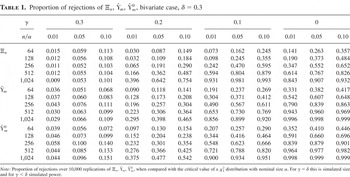
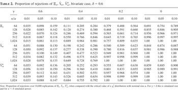
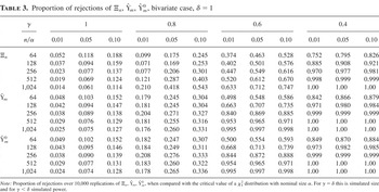
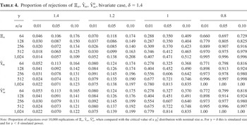
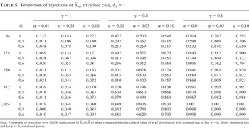
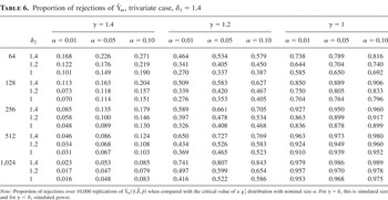
Results of the proportion of rejections over 10,000 replications when comparing the values of the statistic with the α = 0.01, 0.05, 0.10 nominal critical values of the χ₁² distribution are reported in Tables 1, 2, 3, & 4 for the different values of δ. Overall all the three tests are oversized, but in almost all cases sizes react appropriately as n increases. As expected, in terms of size, the parametric test performs best, followed by

, with

being worst, although for cases δ = 1, 1.4, its behavior is very similar to that of

. For the parametric test, sizes are best for δ = 0.3, and it also shows a better performance for the mean-reverting case (δ = 0.6) than for the non-mean-reverting ones (δ = 1, 1.4), the case δ = 1 being worst. The mean-reverting and (asymptotically) stationary cases also favor the semiparametric statistics in terms of size when n is small, but here especially the proportions of rejections corresponding to

do not show a very clear convergence pattern to the nominal sizes as n increases, unlike in the δ = 1, 1.4 cases, where it appears to be a monotonic convergence toward the nominal values. Clearly, the parametric test is most powerful for δ = 0.6, with a very good performance relative to other values of δ for which the reduction of the order of the observables under H₁ is just 0.2 (where indeed the increase of the proportion of rejections as n increases could be very slow). This perhaps indicates that the jump from nonstationary observables to (asymptotically) stationary cointegrating errors (which does not appear for other combinations of δ, γ = δ − 0.2) is important. In terms of power, the semiparametric statistics are comparable to the parametric one (although note that the proportions of rejections are not size corrected). Similarly to the parametric test, the semiparametric tests have also problems detecting the alternative when δ = 1, 1.4 (but not when δ = 0.6) and γ = δ − 0.2, the proportion of rejections being higher here than for the parametric test when n is small, although increasing at a slower rate as n increases. In almost all cases the proportions of rejection react appropriately as n and the cointegrating gap (δ − γ) increase.

Proportion of rejections of Ξn, , , bivariate case, δ = 0.3

Proportion of rejections of Ξn, , , bivariate case, δ = 0.6

Proportion of rejections of Ξn, , , bivariate case, δ = 1

Proportion of rejections of Ξn, , , bivariate case, δ = 1.4

In the second part of the experiment, we analyze the behavior of the semiparametric statistic

, in a multivariate framework (with three observables), with possibly different integration orders. We generated ε_t (see Assumption 1) as a trivariate zero-mean Gaussian white noise with covariance matrix

noting that if A(L) = I₃ in Assumption 1, this covariance structure leads to a white noise u_t with covariance matrix

and so the scenario is similar to that described in the first part of the experiment. However, we introduced further short-memory structure to our design by setting A⁻¹(L) = I₃ − ΦL, Φ = diag(0.5, 0.5, 0.5) and generating w_t accordingly. Then, denoting x_t = (x_1t,x_2t)′, u_xt = (u_x1,t,u_x2,t)′, x_1t, x_2t are generated from the input processes u_x1,t, u_x2,t, as fractionally integrated processes of orders δ₁, δ₂, respectively, where δ₁ = 1.4, 1 and δ₂ = δ₁, δ₁ − 0.2, δ₁ − 0.4. Finally, y_t was generated as in (4) with β = (1,1)′ and

Note that in the present setting, especially when δ₂ < δ₁, the covariance structure of u_t is very distant from that of the white noise situation, and so the use of

instead of

seems more appropriate, although both statistics are, at least to first-order properties, asymptotically equivalent. To compute the statistic and the estimates of the nuisance parameters, we employed the set of bandwidths m = 12, 20, 31, 60, 110, for n = 64, 128, 256, 512, 1,024, respectively. Note that these bandwidths are approximately half of the bandwidths used in the first part of the experiment, and they were chosen on the observation that when short-memory structure is present, smaller bandwidths than in the white noise situation are warranted. The orders δ₀, δ₁, δ₂ are estimated by

,

,

, which are calculated by the same procedure described in the first part of the experiment, from the series y_t, x_1t, x_2t, respectively. Also

where

. Here, note that on the estimation of f we chose bandwidth m/2, because, especially when δ₂ < δ₁, the estimation of f at a particular frequency rapidly gets distorted when incorporating information from frequencies that are relatively far from this particular frequency. As in any semiparametric procedure, the choice of bandwidth is fundamental, and although a more extensive Monte Carlo experiment checking the sensitivity of the test to variations of all bandwidths (and indeed of the short-memory parameters) involved is interesting, our proposed bandwidths give general hints to practitioners on possible choices that behave relatively well.

As mentioned in Section 5, the main issue here is to estimate γ. Following the strategy described there, we compute the NB estimate from the regression of Δy_t on Δx_t and estimate γ from residuals

by the method described in the first part of the experiment, finally obtaining

. Our results are presented in Tables 5 and 6. As in the bivariate case, when n is small our test is clearly oversized (especially for δ₁ = 1.4), although as n increases size reacts in the appropriate direction, and so they are very close to the nominal ones when n = 1,024 (the statistic being in some cases undersized for large n). For small n, a decrease in δ₂ implies a decrease in size, this effect disappearing as n increases. In terms of power, the test behaves in a very similar way for both the δ₁ = 1 and δ₁ = 1.4 cases. Power decreases with δ₂ and reacts appropriately as n increases. The test is able to detect the alternative γ = δ₁ − 0.2 now, although, especially when δ₂ = δ₁ − 0.4, the increase in power as n increases is slow. Overall, we find that the results in this second part of the experiment, which describe a more realistic situation than the first one, are certainly encouraging, noting that for simplicity we neither applied the provision made in Section 5 about the rate of growth of the bandwidth used in the estimation of γ (in comparison to that used in the estimation of β) nor used sophisticated estimates of the nuisance parameters. In fact, estimation procedures of these parameters using bias-reducing devices are readily available (see Hualde and Robinson, 2004), and using them might lead to even better finite-sample results.

Proportion of rejections of , trivariate case, δ1 = 1

Proportion of rejections of , trivariate case, δ1 = 1.4