The overall implementation framework of the proposed method

The framework of the design method is shown in Fig. 1 QGA is initially employed as a data generator to collect potential high-quality data continuously. The topology data obtained by QGA is then converted into the antenna model and sent to HFSS for simulation. Subsequently, E-MLPs, which is used to accelerate the EM simulation, is trained by the dataset with the proposed method. During the optimization, the training dataset for E-MLPs will be continued to collect. Finally, RL is used to optimize the antenna topology. RL can dynamically adjust each decision based on the rewards associated with different actions in the design environment [Reference Su, Yin, Li, Zhao and Yin14, Reference Yang15]. It is worth noting that QGA is only applied in the initial dataset collected stage rather than the final antenna optimized stage. The primary reason is that EAs requires multiple full-wave EM simulations to get the optimal topology solution [Reference Zhou16–Reference Koziel, Pietrenko-Dabrowska and Pankiewicz18].

Figure 1.

The framework of the proposed method.

The method of training dataset construction and processing

In this paper, a high-quality dataset construction method is proposed and its implementation framework is shown in Fig. 2. Compared with traditional orthogonal or random sampling method, the proposed method ensures the quality of the dataset. In addition, during the process of dataset collection, TBM is developed to define the bidirectional conversion between the antenna topology structure and the antenna topology coding matrix, which is aimed to assist the algorithm to identify the antenna topology data. As shown in Fig. 2, the initial antenna topology is decomposed into several basic topology grid units. Then the antenna topology can be reconstructed by adjusting the material distribution of each basic topology grid unit. The antenna topology coding matrix can be expressed as

(1)\begin{equation} X = \begin{pmatrix} x_{11} & \cdots & x_{1n} \\ \vdots & \ddots & \vdots \\ x_{m1} & \cdots & x_{mn} \end{pmatrix}_{m \times n},\quad x_{i,j} \in \{0,1\} \end{equation}

where $n$ and $m$ represent the number of antenna horizontal and vertical topology grid units, respectively. The binary value 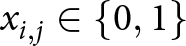$x_{i,j} \in \{0,1\}$ in the matrix $X$ indicates the material coverage state of each grid unit. Specifically, the grid at $(i, j)$ of the antenna has the metal material coverage only when $x_{i,j} = 1$. Each possible antenna topology is stored in the population of QGA, which is composed of several binary value $x_{i,j}$.

Figure 2.

Dataset construction method framework diagram.

Finally, the collected data is processed by using THA. The initial topology matrix is firstly divided into independent components and then augmented along the additional dimension. Through THA, the 2D antenna topology matrix is effectively transformed into a three-channel tensor structure $\ X' $, which is similar to the framework that commonly used in computer vision.

The proposed E-MLPs architecture

In this paper, the proposed E-MLPs adopts the main architecture of MLP-Mixer, which is originally designed for computer vision tasks [Reference Tolstikhin, Houlsby, Kolesnikov, Beyer, Zhai and Unterthiner19]. The special feature of E-MLPs lies in its MLP-based information mixing mechanism. This mechanism avoids expensive convolution or attention-based mechanisms. It efficiently captures global relationships across spatial and feature dimensions [Reference Zhou20, Reference Sharifani and Amini21]. In this work, the proposed E-MLPs is introduced to the field of EM design innovatively, which incorporates three key design modifications as follows.

1) Use the 3D topology tensor as the input data of the model. This special 3D antenna topology tensor can fully utilized the cross-channel information mixing capability of E-MLPs, allowing the topology characteristics of the antenna to be comprehensively captured.

2) Establish a nonlinear mapping from antenna topology to EM response by E-MLPs. The input of E-MLPs is restructured into antenna topology tensors and the EM indicators, such as impedance bandwidth and gain, are obtained from the output layer directly.

3) Build an online optimization mechanism for E-MLPs during the optimization process. In order to enhance the accuracy of the model, E-MLPs is improved with the online learning mechanism. Specifically, the top $n$ best candidates in each iteration are selected for real EM simulation. The simulated results are then added to the dataset to retrain the E-MLPs.

The overall framework of the E-MLPs model is shown in Fig. 3, which consists of three parts. The input data is firstly divided into $M$ complementary overlapping patches by the linear segmentation part and fed into the information mixing part which integrates token mixing layer and channel mixing layer. Token mixing layer establishes associations between different positions in the spatial dimension and integrates features through independent cross-channel operations. Channel-mixing layer realizes feature fusion in the channel dimension and performs cross-channel information interaction for each spatial position. Finally, the prediction and output part is used to fuse high-dimension feature tensors, establishing a direct mapping from the hybrid feature space to the antenna EM performance indicators. Notably, the information mixing layer is only implemented by the MLP, where each MLP comprises two fully connected layers. Each hidden layer contains 1024 neurons with GELU activation applied between the fully connected layers. The operations of token mixing and channel-mixing can be expressed as

(2)\begin{equation} Y^T = X_{*,i} + w_1 \, \text{GELU}\left(w_2 \times \Theta(X'_{*,i})\right), \quad \text{for } i = 1, 2, \dots, Q \end{equation}

(3)\begin{equation} Y^C = Y_{j,*}^T + w_3 \, \text{GELU}\left(w_4 \times \Theta(Y^T_{j,*})\right), \quad \text{for } j = 1, 2, \dots, M \end{equation}

where $\mathbf{Y}^T$ and $\mathbf{Y}^C$ represent the output results of token mixing layer and channel mixing layer, respectively. $\Theta(\cdot)$ is the normalization function, which is used to normalize the input and stabilize the neural network training process. GELU $(\cdot)$ is the activation function, which can be approximated as:

(4)\begin{equation} \text{GELU}(x) = \frac{1}{2}x \left( 1 + \tanh\left( \sqrt{\frac{2}{\pi}} \left( x + 0.044715x^3 \right) \right) \right) \end{equation}

Figure 3.

The framework diagram of E-MLPs.

During the training process, the loss between the predicted results and the real antenna performances is calculated through (5) to guide the process of forward propagation and update the network weights. The loss is defined as:

(5)\begin{equation} \text{Loss}(y_i | \hat{y}_i) = \frac{1}{N} \sum_{i=1}^N \sum_{j=1}^M \left( \frac{y_{i,j} - \hat{y}_{i,j}}{y_{i,j}} \right)^2 \end{equation}

where $N$ denotes the number of samples in each iteration during training. $M$ denotes the number of antenna performance indicators. $y_{i,j}$ and $\hat{y}_{i,j}$ represent the real and prediction antenna performance indicators, such as impedance bandwidth and gain.

The proposed RL architecture

In this work, RL is proposed to optimize the antenna topology based on the deep deterministic policy gradient (DDPG) algorithm. DDPG is a model-free offline policy RL algorithm based on the actor-critic architecture [Reference Silver, Lever, Heess, Degris, Wierstra and Riedmiller22]. The main framework of DDPG-based RL algorithm is shown in Fig. 4.

Figure 4.

The framework diagram of RL.

Actor network performs a certain mapping from the state $s_t$ to the action $a_t$ based on the policy $\mu$. The original actor network parameters $\theta^\mu$ are then updated using the gradient ascent method, which is determined by the gradient of the critic network and its own network. Critic network evaluates state-action pairs $(s_t, a_t)$ to get the Q value function of the current policy and realizes policy evaluation by minimizing the temporal difference error (TD-loss). The parameter of the original critic network $\theta^Q$ is updated by calculating the gradient of TD-loss. In our work, RL is designed to optimize the policy of the algorithm by maximizing the Q-value function which is defined as the future expected discounted reward for a given state-action pair $(s_t, a_t)$. Q-value function can be expressed as follows

(6)\begin{equation} Q(s_t, a_t) = \mathbb{E}\bigl[R_t \bigm| s_t, a_t\bigr] \end{equation}

where $\mathbb{E}[\,\cdot\,]$ denotes the expected value and $R_t$ is the sum of discounted rewards achieved by learning the future steps, which can be calculated by (7).

(7)\begin{equation} R_t = \sum_{k=0}^\infty \gamma^k r_{t+k+1} \end{equation}

where the value of discount factor $\gamma$ is between 0 and 1, which is used to adjust the relative importance of immediate rewards and future rewards. In addition, to enhance the stability of the algorithm, two additional mechanisms, the target network and the experience replay buffer, are added to the DDPG. The target network can stabilize the training process by providing a fixed target for the network, with soft updates applied to both target networks. Through the soft update mechanism, the parameters of the original networks can be inherited by the target networks gradually. The experience replay buffer stores various experiences, including state $s_t$, action $a_t$, reward $r_t$, and next state $s_{t+1}$, which enables the interaction between RL and environment.

In this paper, the algorithm runs for $i$ iterations and each round of iterations runs $T$ steps. The key parameters of RL in the antenna optimization are as follows.

1) Action: Action $a_{t}$ stores the topology information of the antenna. It can be expressed as (8)

(8)\begin{equation} a_{n,t} = \left( \alpha_{1,t}, \alpha_{2,t}, \alpha_{3,t}, \dots, \alpha_{n,t} \right) \end{equation}

where $\alpha_{n,t}$ is the value of each topology grid unit which predicted by the actor network. The antenna topology $X_{t}$ can be obtained by rearranging the action $\alpha_{n,t}$. $\alpha_{n,t}$ can be calculated by

(9)\begin{equation} \alpha_{n,t} = \begin{cases} 1, & \alpha_{n,t} \geq 0.5 \\ 0, & \alpha_{n,t} \lt 0.5 \end{cases} \end{equation}

2) State: The state $s_{t}$ is defined as the performance of the antenna. In this work, in order to reduce the impact of high-dimension curve data on the prediction accuracy, the fitting value of the antenna performance $\Psi_{t}$ is directly stored in the state $s_{t}$.

(10)\begin{equation} s_{t} = \Psi_t = \delta_1 \cdot \sum_{f=f_1}^{f_2} g_1(X_{f}, f) + \delta_2 \cdot g_2(f_0) \end{equation}

where $\delta_{1} \epsilon (1,0)$ and $\delta_{2} \epsilon (1,0)$ are the different personalized weights. They are used to describe the importance of gain and impedance bandwidth, aiming to help RL balance different performance indicators. In this paper, the value of $\delta_{1}$ and $\delta_{2}$ are set to 0.8 and 0.2, respectively. The $g_{2}(f_{0})$ represents the gain value at the target frequency $f_{0}$. Frequency $f_{1}$ and $f_{2}$ are the limit of the target frequency band. In this paper, they are set to 2.30 GHz and 2.60 GHz, respectively. The $g_{1}(X_{t}, f)$ can be defined as

(11)\begin{equation} g_1(X_t, f) = \begin{cases} 1, & \text{if } |S_{11}(X_t, f)| \leq -10\ \text{dB} \\ 0, & \text{otherwise} \end{cases} \end{equation}

where $S_{11}(X_{t},f)$ represents the value of impedance matching when antenna topology $X_{t}$ works at frequency $f$.

3) Reward: Reward $r_{t}$ is a key parameter to update network. The reward function defines the immediate reward that calculated by a certain state. The main goal of the RL is to optimize the action strategy by maximizing the discounted cumulative reward. According to different design performance requirements, reward function should be given to ensure that the next action $a_{t+1}$ can be correctly guided by RL. In this paper, the reward $r_{t}$ is related to the fitting value $\Psi_{t}$, which is designed to be

(12)\begin{equation} r_t = \begin{cases} \dfrac{\Psi_t - \Psi_{t-1}}{\Psi_{\text{thre}}}, & \text{if } \Psi_t \geq \Psi_{\text{thre}} \text{and } \Psi_t \geq \Psi_{t-1} \\ 0, & \text{if } \Psi_{\text{thre}} \lt \Psi_t \leq \Psi_{t-1} \\ -0.1, & \text{if } \Psi_{t-1} \leq \Psi_t \leq \Psi_{\text{thre}} \\ -1, & \text{others} \end{cases} \end{equation}

where $\Psi_{t-1}$ is the fitness value at the previous time step. $\Psi_{thre}$ is the maximum threshold of the fitness value.

Introduction of antenna to be optimized

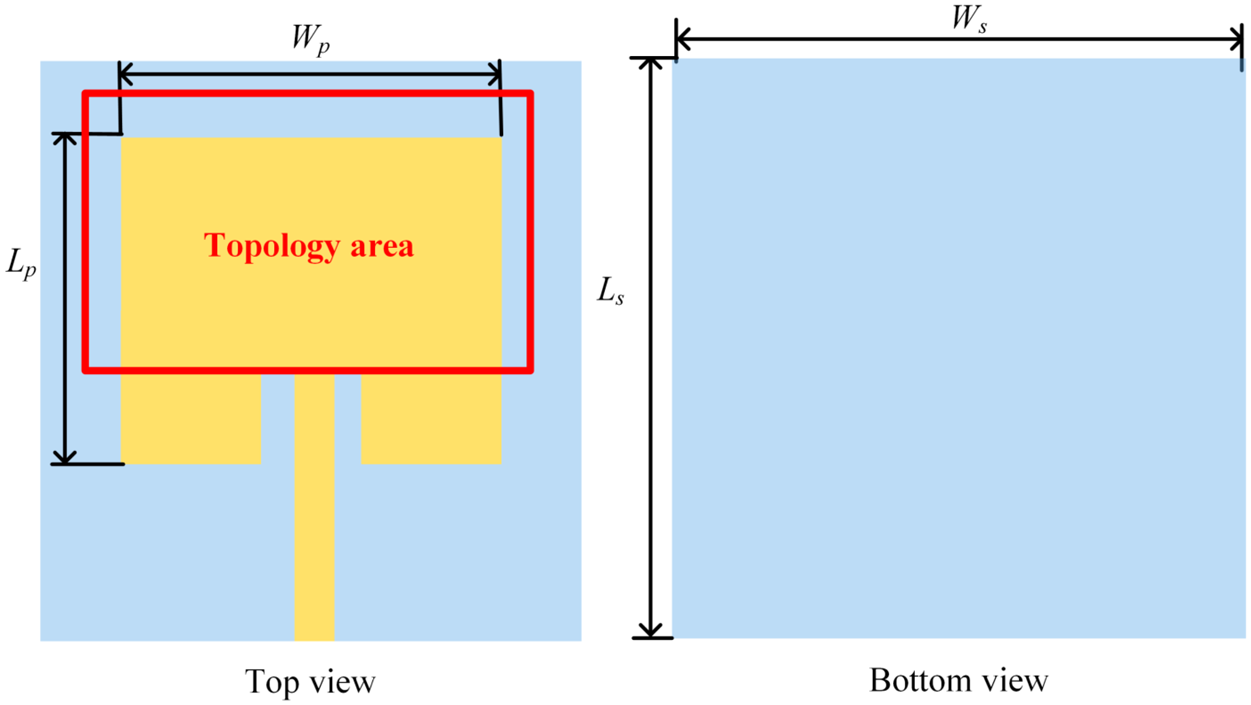
This section takes a miniaturized microstrip patch antenna as an example to verify the effectiveness of the proposed method, which is shown in Fig. 5. The antenna uses a single layer of FR4 epoxy resin as the dielectric substrate. The thickness of the substrate is 1.6 mm, and the relative dielectric constant is 4.4. The length of the patch $W_{p}$ and the width of the patch $L_{p}$ are 34 mm and 29 mm, respectively. The length of the ground $W_{s}$ and the width of the grand $L_{s}$ are 43 mm and 46 mm, respectively. In order to ensure the radiation characteristics of the antenna can be stimulated, the topology area is designed in the square part of the antenna.

Figure 5.

Initial antenna topology diagram.

Experimental environment and algorithm implementation

The entire simulation process is performed on a computer equipped with 128 GB memory and a 2.90 GHz Intel Xeon Platinum processor. The simulation software is ANSYS HFSS 2021R2. To realize conversion between the antenna topology and the antenna topology matrix that defined in TBM, the matrix can be converted into a CAD file and then imported into HFSS. It realizes the automated interaction between the algorithm and HFSS in this paper. Through the sampling method proposed in this paper, 1000 samples are collected for training. The number of design grid units of the antenna is set to 126, with the geometric symmetry constraints applied to the radiation patch. In addition, the original antenna topology is divided into 3 channels through the THA with each channel configured as a 3 $\times$7 grid unit. Finally, the trained E-MLPs is used to replace EM simulation for optimization. During the optimization, 100 iterations is performed in this work, each of iteration has 50 steps. In each iteration, the design results are obtained through E-MLPs and added to the experience reply memory. Then the 10 best candidates are selected for full-wave EM evaluation in the proposed method. The EM simulation results are stored in the dataset and used to retrain the E-MLPs. In addition, in order to speed up the optimization process, the candidate results with zero fitting values are skipped the EM simulation and are directly added to the dataset. This strategy effectively avoids unnecessary EM simulation during the early exploratory phase of RL.

The loss curves for the training and validation results are shown in Fig. 6c. After 100 epochs full training, the training loss dropped around 0.03 and the validation loss remained around 0.1. Fig. 6a and 6b show the comparison between the predicted results and the actual antenna performances of 10 random datasets for the impedance bandwidths and gain values, respectively. It is important to note that both the gain values and impedance bandwidths have been normalized. The results indicate that although there are some variations between the predicted results and actual antenna performances, the overall predicted results can be accepted.

Figure 6.

(a) The performance comparison of E-MLPs prediction results and 10 random samples for normalized |S $_{11}|$ bandwidth. (b) The performance comparison of E-MLPs prediction results and 10 random samples for normalized gain value. (c) The training loss and validation loss of the E-MLPs.

RL optimization results

In this paper, the requirements for antenna optimization are as follows:

1. 1) Target #1: |S $_{11}$| $\leq -$10 dB from 2.40 GHz to 2.50 GHz.

2. 2) Target #2: The operating bandwidth of antenna must include 2.45 GHz.

3. 3) Target #3: The gain at 2.45 GHz must be greater than 1 dBi.

Fig. 7a and 7b show the antenna optimization results in the different optimization stages. Where the target threshold $\Psi_{thre}$ is set to 5. For ease of presentation, three stages, the 1st iteration to the 30th iteration, the 31st iteration to the 60th iteration, and the 61st iteration to the 90th iteration, are referred to stage I, stage II, and stage III, respectively. In stage I, impedance bandwidth is successfully expended by RL. However, its operating frequency band is not the primary frequency band for 5G communication and its gain value at 2.45 GHz is lower than 0 dBi, failing to meet the minimum standard required for the engineering. Therefore, the gain curve of stage I is omitted in Fig. 7b. In stage II, the gain of antenna is significantly improved, but the frequency range when |S $_{11}$| $\leq -$10 still deviates from the target operating frequency. In stage III, the final performance optimization result is achieved by RL, resulting in significant improvement in both gain and impedance bandwidth.

Figure 7.

(a) The optimized results of |S $_{11}$| in different stages. (b) The optimized results of gain in different stages. (c) The average reward of RL. (d) Final optimization results. (e) Antenna topology predicted by RL in different stages.

The change of average reward is shown in Fig. 7c, which matches the RL optimization results of each stage. In stage I, the average reward is low and fluctuates significantly, which indicates that the algorithm is extensively exploring the topology design space. With continuous optimization, the average reward is improved in stage II but notable fluctuations remain, which can be explained by the fact that RL is still in the exploration of the topology space. Finally, the average reward gradually stable and reached the maximum value in stage III. The final optimization results can be also obtained. During the optimization, although the range of reward value during optimization is deeply affected by the design of the reward function, it has no impact on the ability of RL to maximize the cumulative rewards [Reference Papageorgiou, Buzo, Pelz and Noulis23, Reference Zhang24].

The performance comparison between the initial antenna and the optimized antenna is shown in Fig. 7d. The frequency range of |S $_{11}$| $\leq -$10 is expanded from the initial 2.40 GHz-2.43 GHz to 2.43 GHz-2.50 GHz. Compared to the initial topology, the impedance bandwidth has been enhanced by more than 100 $\%$. The gain at 2.45 GHz is improved from the initial 2.55 dBi to 2.90 dBi, representing an approximately 13.7 $\%$ increase. A balance between antenna impedance bandwidth and gain is achieved in the final optimization results. In addition, Fig. 7e further shows the antenna topology optimization result of each stage. As the optimization continues, the topology grid units are gradually concentrated. The final concentrated antenna topology indicates that the gain at 2.45 GHz can be ensured by the large radiating patch area and the improvement of impedance bandwidth can be achieved by the appropriate slotting. The proposed method enables a balance between those contradictory design requirements. Finally, the specific performance comparison of the optimization result in different stages is shown in Table 1.

Table 1.

Performance comparison between the initial and optimization results

Comparison of the proposed method with other methods

In this work, the number of iteration is set to 100, but the optimization standard is achieved after 82 iterations. By using the optimization strategy of skipping the zero fitting value, 116 redundant EM simulation steps are effectively skipped, and 704 EM simulations are actually performed, with a total time of about 35.2 hours. The comparison of optimization results in this paper with other recent related works are shown in Table 2.

Table 2.

Comparison result with other works

Antenna performance optimization is achieved in references [Reference Guler, Karaosmanoglu and Ergul25–Reference Dong, Li and Deng27] by changing the antenna predefined structural templates. Such method offers a high degree of freedom but requires thousands of EM simulations when dealing with the antenna topology problems. In contrast, references [Reference Li, Tang, Cui, Hei and Shi28–Reference Su, Yin, Li, Zhao and Yin30] realize the optimization through fine-tuning antenna parameters. This method requires less time to complete the antenna optimization, but its optimization efficiency is severely restricted by the initial antenna structure and the dimension of the design parameters.

Therefore, this work innovatively applies the RL to the field of antenna topology optimization. Compared with topology optimization method, this study shows an advantage in optimization efficiency. Compared with parameter optimization method, it breaks the inherent constraints of the initial topology and shows a higher degree of freedom. In addition, compared with our previous work [Reference Dou, Gong, Chen, Chen, Shen and Song31, Reference Dou, Gong, Wei, Chen, Chen and Shen32], the proposed method achieves the antenna multi-objective optimization with higher dimension topology data but in less optimization time.

The measurement results of antenna

The experimental sample of the antenna is measured, and the measurement environment is shown in Fig. 8. In addition, Fig. 9 shows the antenna performance comparison of |S $_{11}$| and gain between simulated and measured results. Although there are some differences which may be caused by manufacturing errors and installation differences, the antenna performance is generally consistent. Fig. 10 further shows the measured and simulated results of antenna radiation pattern in the XOZ plane and YOZ plane. The results show that the radiation patterns are also generally consistent.

Figure 8.

Measurement environment of optimized antenna.

Figure 9.

Measurement and simulation results of (a) |S $_{11}$| and (b) gain.

Figure 10.

Measurement and simulation results of radiation pattern in (a) YOZ plane and (b) XOZ plane.