1. Introduction
Global Navigation Satellite System (GNSS) real-time kinematic (RTK) precise positioning and navigation has extensive applications in various fields, such as high-precision monitoring, intelligent transportation and automation equipment (Jiang et al., Reference Jiang, Chen, Chen, Chen, Pan, Liu and Liu2022; Paziewski, Reference Paziewski2020; Won et al., Reference Won, Ahn, Lee, Heo, Sung and Lee2015). Unfortunately, in practical applications, GNSS observations often unavoidably incorporate multiple and mixed abnormal signals, especially in multi-GNSS systems under harsh environments like natural and urban canyons. With the increasing deployment of multi-frequency and multi-constellation GNSS systems, differing signal accuracies and environmental impacts such as reflection, refraction, diffraction, occlusion and interference contribute to a variety of abnormal measurements. In addition, interactions between signals from different systems or frequencies may lead to further inconsistencies. Specifically, these abnormal measurements involve outliers and site-specific unmodeled errors including multipath, diffraction and non-line-of-sight (NLOS) reception (Hsu, Reference Hsu2018; Sun et al., Reference Sun, Zhang, Cheng and Ochieng2022; Zhang et al., Reference Zhang, Li, He, Chen and Li2022, Reference Zhang, Wang and Li2025). These abnormal measurements will significantly affect the precision and reliability of GNSS precise positioning and navigation (Wen et al., Reference Wen, Zhang and Hsu2021; Yuan et al., Reference Yuan, Zhang, He, Wen and Zeng2022). Therefore, how to deal with tricky abnormal measurements remains a complex problem in GNSS data processing. Currently, an important abnormal measurement processing approach is data detection, which can be summarised into two main categories: data checking based on the prior innovation and data snooping based on a posterior residual (PR).
The innovation vector (IV) describes the difference between the actual measurement and the predicted measurement, and it is an indicator that reflects kinematic system disturbance (Yang et al., Reference Yang, He and Xu2001; Zabalegui et al., Reference Zabalegui, De Miguel, Mendizabal and Adin2022). However, the IV may be contaminated due to some factors such as poor observation quality, which leads to inaccuracy in GNSS solutions. Therefore, the IV check procedure is usually an important part of abnormal measurement detection (Mehra and Peschon, Reference Mehra and Peschon1971). Typically, the IV is used to construct testing statistics and this is employed in some practical applications (Crespillo et al., Reference Crespillo, Grosch and Meurer2017; Grosch et al., Reference Grosch, Crespillo, Martini and Günther2017). However, threshold detection of the IV method is commonly employed since it is easy to implement and efficient in practical applications (Takasu, Reference Takasu2009). The performance of the IV check is constrained by the uneven quality of GNSS observations and setting a single constant threshold in the IV check for abnormal measurement removal may lead to inefficient abnormal measurement detection, and inaccurate positioning and navigation results. Consequently, the effectiveness of the IV check is influenced by both observation quality and the definition of thresholds.
The other main approach is the data snooping method (Baarda, Reference Baarda1968), which mainly relies on hypothesis testing to decide between a null and a single or group of alternative hypothesis models (Koch, Reference Koch2015; Lehmann Reference Lehmann2013). These methods are grounded in the functional model according to the formulating hypotheses based on the type, quantity and location of abnormal measurement, and the hypothesis testing statistics obey the normal distribution or others. In the GNSS community, a well-known abnormal measurement detection method has been proposed and widely applied, i.e. the method of detection, identification and adaptation (DIA) (Teunissen, Reference Teunissen2018). However, in practical applications, the DIA method cannot guarantee the complete correctness of test decisions and the unbiasedness of estimated parameters, especially in harsh environments. In addition, the missed detection, the false alarm and the incorrect exclusion are inevitably conducted due to the misspecification models, the geometry conditions of the model, the separability among hypotheses, the selected test statistics and the predetermined critical values of testing, etc. (Lehmann, Reference Lehmann2012; Leick and Emmons, Reference Leick and Emmons1994; Yang et al., Reference Yang, Shen, Li and Rizos2021).
Therefore, using these traditional approaches alone cannot fully meet the needs of GNSS precise positioning and navigation, especially in harsh environments. Moreover, for the problem of multiple and mixed abnormal measurements in multi-GNSS systems, both traditional data checking and traditional data snooping methods will lead to the reduction of positioning accuracy and reliability. Consequently, it is essential to explore the theoretical basis for combining data checking and data snooping methods further, and the accurate combination of the two methods needs to be systematically investigated. In this study, an approach for multiple and mixed abnormal measurement processing in multi-GNSS positioning and navigation based on the resilient a priori innovation and posterior residual in harsh environments is proposed. Although there are some specific abnormal measurement processing approaches based on the a priori innovation and posterior residual (Takasu, Reference Takasu2009), little attention has been paid to how to realise the combination of these two methods with each other for more accurate multiple and mixed abnormal measurement processing. First, based on the theoretical basis, a complete procedure of the proposed approach considering the observation quality is given. Second, a resilient IV (RIV) method is used for data checking. There are two improvements compared with the traditional IV method. The first improvement is that both static and kinematic processing modes are considered when calculating the predicted state vector, thereby it can provide a more reliable innovation vector. The second improvement addresses the potential problem of inappropriate threshold setting, which is achieved by defining corresponding thresholds according to the different pseudorange and phase measurement accuracy of different GNSS systems. Third, a data snooping process based on the resilient PR (RPR) method is implemented. Specifically, the iteration strategy is changed and the total number of redundant observations is considered in the iterative process; thus the data snooping process more accurately combines the observation quality.
The organisation of the following parts is as follows. In the ‘Methodology’ section, the mathematical model of GNSS RTK positioning and conventional abnormal measurement processing methods, including the traditional IV and PR methods, are first introduced. This is followed by a description of the proposed approach for handling multiple and mixed abnormal measurements in multi-GNSS positioning and navigation, based on resilient a priori innovations and posterior residuals. The ‘Experimental setups’ section presents the static and kinematic experimental datasets as well as the settings of resilient parameters. The experimental results and analysis will be elaborated in the ‘Results and discussion’ section. Finally, the conclusion will be drawn in the ‘Conclusion’ section.
2. Methodology
In this section, the mathematical model of GNSS RTK positioning is given first. Then, the strategies of the traditional IV and traditional PR methods are introduced to process abnormal measurements. Finally, a multiple and mixed abnormal measurement processing approach is proposed by considering the quality of the observations, where specific schemes of the RIV and RPR methods are deduced.
2.1. Mathematical model of GNSS RTK positioning
The purpose of the mathematical model is to establish the relationship between observations and the unknown parameters. For RTK positioning and navigation under harsh environments, the operator of between-receiver and between-satellite double differencing is introduced to eliminate the clock errors and hardware delays, and reduce atmospheric delays. The double-differenced (DD) code and phase observations on frequency
 $i$
are usually expressed as (Leick et al., Reference Leick, Rapoport and Tatarnikov2015; Yuan et al., Reference Yuan, He, Zhang, Liu, Li and Jiang2023; Zhang et al., Reference Zhang, Li, He and Hsu2023c)
 $$\nabla \Delta P_{br,i}^{mn} = \nabla \Delta \rho _{br}^{mn} + \nabla \Delta I_{br,i}^{mn} + \nabla \Delta T_{br}^{mn} + \nabla \Delta U_{br,i}^{mn} + \nabla \Delta {\rm{{\rm Z}}}_{br,i}^{mn}$$
 $$\nabla \Delta {\rm{\Phi }}_{br,i}^{mn} = \nabla \Delta \rho _{br}^{mn} + {\lambda _i}\nabla \Delta N_{br,i}^{mn} - \nabla \Delta I_{br,i}^{mn} + \nabla \Delta T_{br}^{mn} + \nabla \Delta u_{br,i}^{mn} + \nabla \Delta \zeta _{br,i}^{mn}$$
where ‘
 $\nabla $
’ and ‘
 $\Delta $
’ are operators that express the between-satellite and between-receiver differences, respectively; superscripts ‘
 $m$
’ and ‘
 $n$
’ denote the reference and common satellites, respectively; subscripts ‘
 $b$
’ and ‘
 $r$
’ denote the base and rover receivers, respectively;
 $P$
and
 ${\rm{\Phi }}$
denote the code and phase observations, respectively;
 $\rho $
and
 $\lambda $
denote the receiver-satellite range and wavelength, respectively;
 $I$
and
 $T$
denote the ionospheric and tropospheric delays, respectively;
 $U$
and
 $u$
denote the code and phase unmodeled effects mainly including multipath errors, respectively;
 ${\rm{{\rm Z}}}$
and
 $\zeta $
denote the observation noise of code and phase observations, respectively; and
 $N$
denotes the integer ambiguity. In general, the GNSS DD mathematical model can be deduced as
 $$\left[ {\matrix{ P \cr \phi \cr } } \right] = \left[ {\matrix{ {{e_f} \otimes {A_k}} & 0 \cr {{e_f} \otimes {A_k}} & {{B_f} \otimes {I_s}} \cr } } \right]\left[ {\matrix{ x \cr N \cr } } \right] + \left[ {\matrix{ {\rm Z} \cr \zeta \cr } } \right]$$
 $${D = \left[ {\matrix{ {{Q_{PP}}} & {{Q_{P\phi }}} \cr {{Q_{\phi P}}} & {{Q_{\phi \phi }}} \cr } } \right]}$$
with
 $P \!= \!{\left[ \!{P_1^{\rm{T}}, \cdots, P_f^{\rm{T}}} \!\right]^{\rm{T}}}\!$
,
 ${P_f} \!= \!{\left[ \!{\nabla \Delta P_{br,\, f}^{m1}, \cdots, \nabla \Delta P_{br,\, f}^{mn}} \! \right]^{\rm{T}}}$
;
 $\phi \!= \!{\left[ \!{\phi _1^{\rm{T}}, \cdots, \phi _f^{\rm{T}}} \! \right]^{\rm{T}}}\!$
,
 ${\phi _f} \!= \!{\left[ \!{\nabla \Delta \phi _{br,\, f}^{m1}, \cdots, \nabla \Delta \phi _{br,\, f}^{mn}} \right]^{\rm{T}}}$
;
 ${\rm Z} = {\left[ \!{{\rm Z}_1^{\rm{T}}, \cdots, {\rm Z}_f^{\rm{T}}} \!\right]^{\rm{T}}}$
,
 ${{\rm Z}_f} = {\left[ \!{\nabla \Delta {\rm Z}_{br,\, f}^{m1}, \cdots, \nabla \Delta {\rm Z}_{br,\, f}^{mn}} \!\right]^{\rm{T}}}$
;
 $\zeta = {\left[ {\zeta _1^{\rm{T}}, \cdots, \zeta _f^{\rm{T}}} \right]^{\rm{T}}}$
,
 ${\zeta _f} = {\left[ {\nabla \Delta \zeta _{br,\, f}^{m1}, \cdots, \nabla \Delta \zeta _{br,\, f}^{mn}} \right]^{\rm{T}}}$
;
 $N = {\left[ {N_1^{\rm{T}}, \cdots, N_f^{\rm{T}}} \right]^{\rm{T}}}$
,
 ${N_f} = {\left[ {\nabla \Delta N_{br,\, f}^{m1}, \cdots, \nabla \Delta N_{br, \, f}^{mn}} \right]^{\rm{T}}}$
, where
 ${A_k}$
denotes the
 $k \times 3$
design matrix of
 $x$
;
 ${B_f} = {\rm{diag}}\left( {{\lambda _1}, \cdots, {\lambda _f}} \right)$
denotes the design matrix of
 $N$
;
 ${e_f}$
and
 ${I_s}$
denote the
 $f$
-row vector with all ones and
 $s \times s$
identity matrix, respectively; subscript ‘
 $f$
’ denotes the index of frequency;
 $x$
and
 $N$
denote the unknown coordinate components and integer ambiguities, respectively;
 ${\rm Z}$
and
 $\zeta $
denote the code and phase observations noise, respectively; and operators ‘
 $ \otimes $
’ and ‘
 ${\rm{diag}}$
’ denote the Kronecker product and diagonal concatenation of elements, respectively. Here,
 $D$
denotes the variance-covariance matrix of GNSS observations;
 ${Q_{PP}}$
and
 ${Q_{\phi \phi }}$
denote the variance-covariance matrices of
 $P$
and
 $\phi $
, respectively. Based on Eq. (3), the GNSS functional model can be simplified as
 $$L = AX + E$$
where
 $L$
denotes the observation vector;
 $A$
denotes the design matrix of unknown parameters;
 $X$
denotes the coordinate components and ambiguities; and
 $E$
denotes the observation noise and residual observation error vector.
2.2. Traditional IV and traditional PR methods
In GNSS data processing, the IV check is a key step for excluding abnormal measurements, which aids in the removal of multiple and significant abnormal measurements to enhance positioning and navigation accuracy. The innovation vector
 ${\bar V_t}$
and predicted state vector
 ${\bar X_t}$
at epoch
 $t$
can be expressed as (Yang, Reference Yang2006)
 $${\bar V_t} = {A_t}{\bar X_t} - {L_t}$$
 $${\bar X_t} = {{\it \Phi} _{t,t - 1}}{\hat X_{t - 1}}$$
where
 ${A_t}$
and
 ${L_t}$
denote the design matrix and measurement vector at epoch
 $t$
, respectively;
 ${\Phi _{t,t - 1}}$
denotes the transition matrix from epoch
 $t - 1$
to
 $t$
;
 ${\hat X_{t - 1}}$
denotes the estimated state vector at epoch
 $t - 1$
. Therefore, to control the impact of abnormal measurements and abnormal state prediction information on the estimation of state parameters, each element in the innovation vector
 $\bar V$
needs to be checked. The traditional IV check method of eliminating abnormal measurements is to set a constant threshold
 $\omega $
, then compare each element in
 $\bar V$
against
 $\omega $
. If one element of
 ${\bar V}$
is found to be larger than the
 $\omega $
, the corresponding element in
 $L$
is regarded as an abnormal measurement and then deleted.
Additionally, after parameter estimation, the residual vector
 ${\hat v_t}$
at epoch
 $t$
can be expressed as (Yang, Reference Yang2006)
 $${\hat v_t} = {A_t}{\hat X_t} - {L_t}$$
Therefore, the PR check is also a very important procedure for eliminating abnormal measurements in GNSS data processing. Such a procedure then usually consists of the following three steps of detection, identification and adaptation (Baarda, Reference Baarda1968; Zhang et al., Reference Zhang, Li, Yuan and Luo2023b).
Detection: A global test is performed to diagnose whether an error has occurred. The statistic
 ${T_q}$
can be expressed as
 $${T_q} = \hat vQ_{ll}^{ - 1}\hat v$$
where
 $\hat v$
denotes the residual vector; subscript ‘
 $q$
’ denotes the number of redundant observations;
 ${Q_{ll}}$
denotes the variance-covariance matrix of observations. For the statistic
 ${T_q}$
, the chi-square test is used to perform hypothesis testing. Given the significance level
 $\delta $
. If
 ${T_q} \gt \chi _\delta ^2\left( {q,0} \right)$
, the alternative hypothesis is accepted, which indicates that the observations contain abnormal measurements, and then the Identification step is entered. If
 ${T_q} \le \chi _\delta ^2\left( {q,0} \right)$
, the null hypothesis is accepted, which indicates that there are no abnormal measurements in the observations, and then the DIA procedure is skipped.
Identification: Use standardised residuals to construct the
 ${w_g}$
statistic which can be expressed as
 $$\left| {{w_g}} \right| = \left| {{{C_g^{\rm{T}}Q_{ll}^{ - 1}\hat v} \over {\sqrt {C_g^{\rm{T}}Q_{ll}^{ - 1}{Q_{\hat v\hat v}}Q_{ll}^{ - 1}{C_g}} }}} \right|$$
where
 ${C_g} = \left[ {0, \cdots, 0,1,0, \cdots, 0} \right]_{1 \times o}^{\rm{T}}$
,
 $o$
denotes the total number of observations;
 ${Q_{\hat v\hat v}}$
denotes the cofactor matrix of the residuals, satisfying
 ${Q_{\hat v\hat v}} = {Q_{ll}} - A{\left( {{A^{\rm{T}}}Q_{ll}^{ - 1}A} \right)^{ - 1}}{A^{\rm{T}}}$
. Here,
 $A$
denotes the design matrix of the mathematical model and its specific expression can be found in Eq. (3). The
 ${w_g}$
test statistic obeys the standard normal distribution, satisfying
 ${{w_g \,} {\unicode{x223C}} \,N\left( {0,1} \right)}$
. Therefore, find the maximum value
 $\left| {{w_j}} \right|$
in the test statistic
 $\left| {{w_g}} \right|$
. If
 $\left| {{w_j}} \right| \gt {\mu _{{\vartheta \over 2}}}$
, where
 ${\mu _{{\vartheta \over 2}}}\left( {0,1} \right)$
denotes the critical value of the standard normal distribution with significance level
 $\vartheta $
, of which the value is usually 0.05 (Jin and Zhang, Reference Jin and Zhang2025; Zhang et al., Reference Zhang, Yuan, He, Li and Geng2023e). It indicates that the
 ${l_j}$
is most probably an abnormal measurement which will be eliminated. In practical applications, Eq. (10) can be simplified as (Teunissen, Reference Teunissen2006)
 $$\left| {{w_g}} \right| = \left| {{{\hat v} \over {\sqrt {{Q_{\hat v\hat v}}\left( {i,i} \right)} }}} \right|$$
where
 $i$
denotes the index of the
 $i$
th observation.
Adaptation: Use the remaining observations to perform the parameter estimation to obtain reliable results.
Therefore, in the traditional PR method, after eliminating the abnormal measurement
 ${l_j}$
in the Identification step of the DIA method, it returns to the Detection step for the global test to determine whether abnormal measurements still exist. Only after accepting the global test statistics, the data snooping procedure will stop and enter the Adaptation step.
2.3. Proposed method based on the resilient a priori innovation and posterior residual
In this study, an approach for multiple and mixed abnormal measurement processing in multi-GNSS positioning and navigation based on the resilient a priori innovation and posterior residual is proposed for the GNSS harsh environments. The flowchart is shown in Figure 1, where the blue and green panels denote the parts of the RIV method and RPR method, respectively. As shown in the figure, after data preprocessing, the RIV method is first employed to test the innovation vector, aiming to eliminate potential large-magnitude abnormal measurements. Subsequently, parameter estimation is performed to obtain the residuals, which are then subjected to iterative testing using the RPR method to identify and remove remaining small-magnitude abnormal measurements. Finally, reliable GNSS positioning solutions are output.
Flowchart of enhanced abnormal measurement processing approach based on the RIV and RPR methods. The blue and green panels denote the parts of the RIV and RPR methods, respectively.

For the RIV method, how to accurately and resiliently update the IV for different positioning applications is the first key procedure. According to Eq. (6), the value of innovation vector
 ${\bar V_t}$
is related to the predicted state vector
 ${\bar X_t}$
. In GNSS data processing, the predicted state vector
 ${\bar X_t}$
is usually updated by the Extended Kalman Filter (EKF) strategy for the kinematic processing mode (Takasu, Reference Takasu2009). However, anomalies in the state or observations at a single epoch may still propagate through the standard prediction model, introducing errors into subsequent epochs. This contamination may render the innovation vector less reliable, thereby compromising positioning accuracy. Such effects are especially detrimental in static positioning scenarios, where high precision and reliability are critical. Moreover, in the static processing mode, especially in monitoring situations, the coordinates of the rover station are almost constant between adjacent epochs. Additionally, for the GNSS positioning solutions, it is noted that the positioning accuracy of the fixed solution is generally higher than that of the float solution (Li et al., Reference Li, Shen, Feng, Gao and Yang2014; Teunissen, Reference Teunissen1997). This difference in accuracy also affects the computation of the innovation vector and the reliability of subsequent abnormal measurement detection. Based on this, the RIV method makes resilient modifications to the predicted state vector
 ${\bar X_t}$
. Specifically, the predicted value
 ${\bar X_t}$
is improved as
 $$\bar X_t^\epsilon = \left\{ {\matrix{ {{{ \check X_i^\epsilon + \cdots + \check X_{t - 1}^\epsilon } \over {{N^\epsilon }}},\;\;{D_{t - 1}} \le \theta } \cr {\bar X_{t - 1}^\epsilon, \;\quad\quad{D_{t - 1}} \gt \theta } \cr } } \right.$$
 $$\bar X_t^\epsilon = \left\{ {\matrix{ {{{\check X_i^\epsilon + \cdots + \check X_{t - 1}^\epsilon } \over {{N^\epsilon }}},\;\;{D_{t - 1}} \le \theta } \cr {X_{t - 1}^\epsilon, \;\quad\quad{D_{t - 1}} \gt \theta } \cr } } \right.$$
where
 ${\check X_i}\;\left( {i = 1,2, \ldots .,t - 1} \right)$
denotes the GNSS solution vector at epoch
 $i$
; superscripts ‘
 $\varepsilon $
’ and ‘
 $\epsilon $
’ denote the fixed and float solutions, respectively;
 ${D_{t - 1}} = \sqrt {{{\left( {\check X_{t - 1}^x - \bar X_{t - 1}^x} \right)}^2} + {{\left( {\check X_{t - 1}^y - \bar X_{t - 1}^y} \right)}^2} + {{\left( {\check X_{t - 1}^z - \bar X_{t - 1}^z} \right)}^2}} $
, where the superscripts ‘
 $x$
’, ‘
 $y$
’, ‘
 $z$
’ denote three directions, respectively;
 $\theta $
denotes a constant threshold. It should be emphasised that if the value of
 ${D_{t - 1}}$
exceeds the threshold
 $\theta $
, the
 ${\check X_{t - 1}}$
will be excluded in the future calculation of
 $\bar X$
. Thus, the
 $N$
denotes the number of
 ${\check X_i}$
that remain after the exclusions. Consequently, Eqs. (12) and (13) represent the schemes for predicting
 ${\bar X_t}$
based on fixed and float solutions, respectively.
In the RIV method, the first level of classification distinguishes between innovation vectors derived from fixed and float solutions, as their prediction accuracy differs significantly. Based on this classification, two sets of innovation vectors are computed separately and independently used for observation screening. Additionally, according to Eq. (6), in both static and kinematic processing modes, the value of the innovation vector
 ${\bar V_t}$
is also related to the measurement vector
 ${L_t}$
. It should be noted that harsh environments will deteriorate the quality of observation data, where multiple and mixed abnormal measurements often occur (Zhang et al., Reference Zhang, Yuan, He, Li and Geng2023e). The observation quality is discrepant between different GNSS systems (Dach et al., Reference Dach, Schaer, Lutz, Meindl and Beutler2010). Moreover, the accuracy of pseudorange and phase observations are also different (Ashkenazi et al., Reference Ashkenazi, Moore and Westrop1991; Zhang and Wang, Reference Zhang and Wang2025). Therefore, within each prediction type (fixed or float), the RIV method further classifies the observations by the GNSS system (e.g. GPS and BDS) and by observation type (pseudorange and phase), resulting in a total of eight categories. To set appropriate thresholds for each category, empirical scaling coefficients are applied based on the standard deviations of the corresponding observation noise. The detailed explanation of the threshold and coefficient values is provided in the experimental settings section. However, the challenge is to select an indicator that can truly reflect the quality of the observed data and correspond effectively to the proposed resilient classification. Pseudorange noise and phase noise can reflect the quality of the corresponding observations. Hence, the RIV method uses the pseudorange and phase random noise standard deviation (STD) values of GNSS systems as parameters for threshold calculation. Specifically, the between-epoch triple-differenced method was employed to calculate pseudorange and phase noise in this study (Li et al., Reference Li, Zhang, Li, Luo and Ferreira2023). Then twice the mean square error value of the noise is used to eliminate some obvious outliers. The STD value of pseudorange noise or phase noise
 ${{\rm{\Omega }}_j}$
at frequency
 $j$
can be described as (Teunissen and Montenbruck, Reference Teunissen and Montenbruck2017)
 $${\Omega _j} = \sqrt {{1 \over {8 \times \left( {{N_{{\rho _j}}} - 1} \right)}}\sum\limits_{u = 1}^{{N_{{\rho _j}}}} {{{\left( {\Delta \Delta {\Delta _{{\rho _j}}}\left( {{t_u}} \right) - \overline {\Delta \Delta {\Delta _{{\rho _j}}}\left( t \right)} } \right)}^2}} } $$
where
 ${N_{{\rho _j}}}$
denotes the number of triple differences in pseudorange or phase observations at frequency
 $j$
after eliminations;
 ${\rm{\Delta \Delta }}{{\rm{\Delta }}_{{\rho _j}}}$
denotes the triple differences in pseudorange or phase observations at frequency
 $j$
after eliminations; and
 ${\overline {{\rm{\Delta \Delta }}{{\rm{\Delta }}_{{\rho _j}}}\left( t \right)}}$
denotes the mean value of triple differences in pseudorange or phase observations at frequency
 $j$
after eliminations. Furthermore, the average of the STD values of pseudorange noise or phase noise at all frequencies in one system is used as the STD value of the pseudorange noise or phase noise of the system.
For the RPR method, how to resiliently conduct the residual checks is the key issue. In practical applications, the traditional PR method has the risk of excessively excluding measurements, which may cause a decrease in model strength and failure of ambiguity resolution. Therefore, to enhance the performance and reliability of the DIA procedure, the RPR method makes two improvements compared with the traditional PR method. The first one is that due to the presence of multiple and mixed abnormal measurements that may occur simultaneously, the residuals may not be sufficiently accurate at the first time. Hence, the adaptation will be conducted after each detection and identification in the RPR method. The second one is that to prevent the DIA method from excessively excluding observations and causing discontinuities in the GNSS solution, a resilient threshold
 ${H_t}$
was set at epoch
 $t$
for the maximum number of iterations in the data snooping process, which can be expressed as
 $${H_t} = {q \over \sigma }$$
where
 $q$
denotes the number of redundant observations;
 $\sigma $
denotes a constant value. The data snooping procedure is stopped when the global test statistic is accepted or the count of iterations meets the
 ${H_t}$
. Then the final solution is outputted.
3. Experimental setups
In this section, the experimental setups of the three dedicated datasets are introduced. Then, considering the pseudorange noise and phase noise of the receiver, the setting of the IV thresholds is comprehensively analysed.
3.1. Description of field tests
To investigate the positioning accuracy and stability of the proposed resilient processing methods, three experimental datasets were designed, including two static experimental datasets and one kinematic experimental dataset.
The GNSS data of two static experimental datasets are obtained from two real-time kinematic landslide monitoring stations in Zhejiang, China. The observation conditions of these two datasets are not sufficiently good, which will be described in more detail below. Figure 2 shows the monitoring receiver used for the static monitoring experiment, which was manufactured by High Gain. It consists of a positioning board, a network board and an antenna (Li et al., Reference Li, Zhang, He, Yuan and Zang2022). The sampling interval of the two datasets was 5 s.
Monitoring receiver.

Figure 3 shows the changes in the number of satellites of the two datasets No. 1 and No. 2, where GPS, BDS and total satellites are shown in blue, green and red, respectively. There are 24 hours of observation data for the No. 1 and No. 2 datasets. The number of GPS satellites in both datasets is less than the number of BDS satellites, but the total number of satellites is more than 19, which meets the positioning requirements.
Number of satellites for datasets No. 1 (top) and No. 2 (bottom).

Figure 4 illustrates the position dilution of precision (PDOP) values for two datasets. Most PDOP values fluctuate between 1 and 3, so the spatial distribution of satellites is found to be acceptable. However, there are still some sudden fluctuations, especially in GPS, with some values that can reach over 10. These fluctuations may lead to some multiple and mixed abnormal measurements, which can affect the final positioning results. Therefore, combined with Figure 3, it can be found that the observation data quality of the No. 1 and No. 2 datasets are poor and relatively poor, respectively.
PDOP values for datasets No. 1 (top) and No. 2 (bottom).

One kinematic experimental dataset of 4 minutes and 19 seconds (GPS time 02:21:47–02:26:06) was collected with a sampling interval of 1 s on DOY 130, 2023. Figure 5 shows the kinematic experimental setup, which consists of a GNSS/inertial navigation system (INS). It includes two high-end geodetic receivers and one high-precision microelectromechanical system integrated navigation receiver, all manufactured by CHCNAV (Zhang et al., Reference Zhang, Li and Yuan2023a).
Kinematic experimental setups.

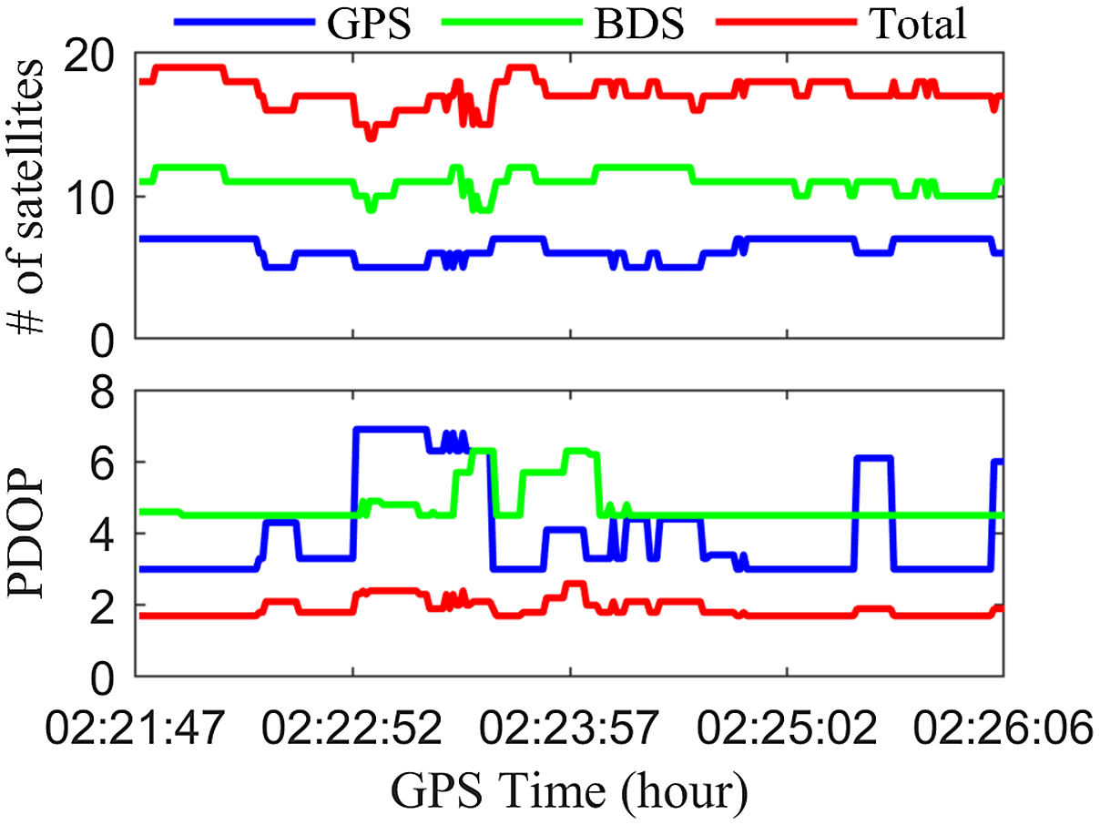
Figure 6 displays a realistic situation of the kinematic experiment in Jiangsu, China. It can be observed that the test case is obscured by many trees and some high buildings. In addition, Figure 7 illustrates the number of satellites and PDOP values for dataset No. 3. The total number of satellites can all reach more than 14, which satisfies the basic positioning and navigation requirements, and the PDOP values are concentrated between 3 and 5, with some peaks up to 6.9; thus leading to some multiple and mixed abnormal measurements which influence the positioning and navigation results.
One real situation of the kinematic experiment for dataset No. 3.

Number of satellites and PDOP values for dataset No. 3.

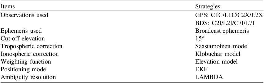
Additionally, all experiments were performed by our self-developed software C-RTK (Canyon RTK), Table 1 presents the detailed processing strategies. By using the L1 and L2 frequencies of GPS, and the B1 and B2 frequencies of BDS to calculate the pseudorange noise and phase noise of the two systems, respectively, the parameters for the thresholds computation of the RIV method are provided. The baseline solutions are estimated using the EKF strategy, which generates the innovation vector during the time update and measurement update process. It must be emphasised that the innovation vector for the RIV method in the static experiments is different, as explained in detail in the Methodology section.
RTK common processing strategies

3.2. Determination of resilient parameters
As aforementioned, to conduct the IV check, the thresholds need to be set precisely. Therefore, the
 $\omega $
was set to 4 m in the traditional IV method, and the
 $\theta $
was set to 2 m and 4 m for the fixed and float solution in the RIV method, respectively. However, to proceed with the RIV method, the pseudorange noise and phase noise STD values for each station need to be first calculated by using Eq. (14), and then the resilient thresholds are adjusted by the relevant coefficients.
Figure 8 shows the pseudorange noise for dataset No. 1 at two frequencies of the GPS and BDS systems, respectively. The pseudorange noise STD values at L1 and L2 frequencies of GPS are calculated as 0.579 m and 0.566 m, respectively. Thus, the pseudorange noise STD value of GPS for dataset No. 1 is 0.573 m. Similarly, the pseudorange noise STD values at B1 and B2 frequencies of BDS are calculated as 0.551 m and 0.427 m, respectively, resulting in a pseudorange noise STD value of BDS for dataset No. 1 of 0.489 m. However, due to some jumps in the clock error of the receiver in the carrier phase observations, the phase noise calculated by the between-epoch triple-differenced method appears falsely high, so the standard deviation values of phase noise were determined based on the pseudorange noise standard deviations. Specifically, the carrier phase measurement noise is very small, typically at a millimetre level, and usually taken as 1/100 of the pseudorange measurement noise (Hofmann-Wellenhof et al., Reference Hofmann-Wellenhof, Lichtenegger and Wasle2007). It is worth noting that if the accurate estimation of the stochastic characteristics of a station is required, there are some alternative methods (Zhang et al., Reference Zhang, Li, Shen and Yang2017, Reference Zhang, Yuan, He, Chen and Zhang2023d). Therefore, the GPS phase noise STD value for dataset No. 1 is 5.73 mm and the BDS phase noise STD value for dataset No. 1 is 4.89 mm.
The panels from top to bottom denote the pseudorange noise (m) at GPS L1, GPS L2, BDS B1 and BDS B2 frequencies for dataset No. 1. The red dotted lines denote twice the mean square error values of the noise at each frequency.

Table 2 shows the STD values of pseudorange noise and phase noise in GPS and BDS systems for datasets No. 1 to No. 3. The pseudorange noise STD values and phase noise STD values are different depending on the different experimental setups and experimental environments of the datasets, and these values reflect the quality of the observed data, which play a significant role in enabling the RIV method to reject abnormal measurements effectively.
GPS/BDS pseudorange noise and phase noise STD values for datasets No. 1 to No. 3

Considering the consistency between the thresholds and the noise STD values, three coefficients were established to adjust the eight thresholds associated with the fixed and float solutions. Specifically, the construction of the eight thresholds is based on the classification of observations by prediction type (fixed or float), GNSS system (GPS or BDS) and observation type (pseudorange or phase). First, for the innovation vectors derived from the fixed solution, the coefficient
 $\alpha $
is applied to scale the STD values of pseudorange observation noise for each GNSS system, thereby determining the pseudorange-related thresholds. Second, the coefficient
 $\beta $
is applied similarly to scale the STD values of phase observation noise, yielding the corresponding thresholds for phase observations. Third, since float solutions generally have lower positioning accuracy and greater uncertainty than fixed solutions, the coefficient
 $\gamma $
is used as a unified scaling factor applied to the thresholds originally determined from the fixed solution-based innovation vectors. This allows the method to tolerate larger deviations when evaluating observations predicted from float solutions. In harsh environments, where observation quality further degrades, all coefficients can be appropriately enlarged to increase robustly against frequent and mixed outliers.
Therefore, for the four thresholds of the fixed solution, in the static experiment, the thresholds can be set small due to the minimal changes in the position of the monitoring station, so the
 $\alpha $
and
 $\beta $
values are set to 1 and 10, respectively. For the four thresholds of the float solution, due to the limited accuracy of float solutions, the
 $\gamma $
value is always 20 in both static and kinematic experiments. However, in the kinematic experiment, since only resilient classification of observations is performed, the thresholds of the fixed solution for different systems are used as the corresponding thresholds of observations. In addition, due to the continuous changes in the position of the monitoring station and the harsh experiment environments, the
 $\alpha $
and
 $\beta $
values are set to 10 and 100, respectively. Additionally, to conduct the RPR check, the constant value
 $\sigma $
were defined as 3 and 5 in static and kinematic experiments, respectively.
4. Results and discussion
In this section, a comprehensive analysis of the positioning results obtained by different methods for both static and kinematic experiments was conducted, and presented the performance of the proposed resilient processing methods under harsh conditions. Thus, the effectiveness and reliability of the processing approach are clarified.
4.1. Analysis of the static experiments
The performances of the RIV and RPR methods were investigated in static experiments. The GNSS observations from two datasets, characterised by poor and relatively poor data quality, were processed using seven different methods, including without IV and PR (WIP); traditional IV (TIV); traditional PR (TPR); traditional IV and PR (TIP); RIV; RPR; and resilient IV and PR (RIP) methods. The results of the seven methods were carefully analysed and compared in terms of ambiguity resolution, positioning bias and accuracy. Here, the STD values of the positioning errors with respect to the reference benchmarks were calculated to evaluate the positioning accuracy.
Figure 9 shows the ambiguity success rates of the seven methods for the two datasets. The results of the TIV, RIV, TPR, RPR, WIP, TIP and RIP methods are represented in light blue, orange, black, purple, green, dark blue and red, respectively. First, it can be found that compared with the TIV method, the RIV method increases the ambiguity success rates of the two datasets No. 1 and No. 2 by 14.9% and 5.1%, respectively. Second, compared with the TPR method, the RPR method improves the ambiguity success rate by 2.6% in dataset No. 2. However, the ambiguity success rate in dataset No. 1 with poor observation data quality of the RPR method is reduced, whereas the positioning accuracy is improved which will be shown later. It indicates that the fixed ambiguities are not correct in the TPR method, thus proving the superiority of the resilient setting in the RPR method. Third, compared with the WIP and TIP methods, the RIP method has significantly improved the ambiguity success rate in the two datasets. Specifically, the improved percentages are 14.1% and 4.7% compared with the TIP method in datasets No. 1 and No. 2, respectively. Additionally, it can be noticed that compared with the other six methods, the RIP method exhibits the highest ambiguity success rates in the two datasets. Hence, the RIP method can improve the performance of ambiguity resolution and has superior reliability.
Ambiguity success rates for datasets No. 1 (top) and No. 2 (bottom).

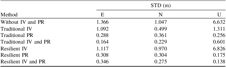
Figure 10 illustrates the positioning results in the east (E), north (N) and up (U) directions of the seven methods for dataset No. 1 with poor observation data quality. The corresponding positioning accuracies are listed in Table 3. Specifically, the percentages of three-dimensional (3D) positioning bias less than 0.1 m from the WIP, TIV, TPR, TIP, RIV, RPR and RIP methods are 7.4%, 23.2%, 78.4%, 82.1%, 54.0%, 91.3% and 88.4%, respectively. The corresponding STD values are 6.852, 1.778, 0.528, 0.664, 6.984, 0.467 and 0.463 m. First, it can be found that compared with the TIV method, the positioning results can be improved by using the RIV method, especially for those results in the purple dotted rectangles. However, as we know, the abnormal measurement processing is not an easy task due to the type, number and location of abnormal measurement in GNSS observations (Huber, Reference Huber1992). Hence, the positioning results of the RIP method seem to be not much improved in the partial processing section, which also leads to some extreme values, resulting in low positioning accuracy in the U direction, which should be further investigated in the future. Second, compared with the TPR method, the positioning errors of the RPR method are smaller in most stages and an improved percentage of 11.6% for 3D positioning accuracy is observed. Moreover, the TPR method achieves higher positioning accuracy than the TIV method. This is because a posterior residuals are computed after parameter estimation, which incorporates the latest observation information. As a result, the estimation of measurement errors becomes more accurate, and abnormal measurements that might have been overlooked are more likely to be identified and excluded. However, this advantage is also dataset-dependent, as the effectiveness of posterior-residual-based strategies can vary with the characteristics of the measurement errors and observation quality. Third, compared with the TIP method, the positioning results are smoother and steadier by using the RIP method, and the improved percentage of 30.2% for 3D positioning accuracy is achieved. Additionally, compared with the other six methods, the RIP method exhibits approximately 50.7% improvement in 3D positioning accuracy on average. Therefore, the RIP method demonstrates extremely superior positioning accuracy.
The panels from top to bottom denote the RTK positioning results of the E (top), N (middle) and U (bottom) directions for dataset No. 1.

STD values by seven different methods for dataset No. 1

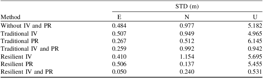
Figure 11 presents the positioning results in the E, N and U directions of the seven methods for dataset No. 2 with relatively poor observation data quality. The corresponding STD values are shown in Table 4. Specifically, the percentages of 3D positioning errors less than 0.1 m for the WIP, TIV, TPR, TIP, RIV, RPR and RIP methods are 56.6%, 69.1%, 89.1%, 98.3%, 86.2%, 92.5% and 99.9%, respectively. The corresponding STD values are 5.295, 5.080, 6.172, 1.392, 5.825, 5.480 and 0.585 m, respectively. First, the RIV method consistently provides highly accurate positioning results throughout most stages, whereas the positioning errors of the TIV method are still large. Specifically, the RIV method performs better on extreme positioning errors. In the E, N and U directions, the extreme values of the RIV method are −2.701, 7.459 and 29.447 m, respectively, while the TIV method reaches −7.442, 19.894 and 51.304 m, respectively. Second, the RPR method still performs excellently compared with the TPR method, especially in the N and U directions, where the positioning accuracies are improved by 73.2% and 11.2%, respectively, and the 3D positioning accuracy is improved by 11.2%. Third, the RIP method still demonstrates better performance than the TIP method, with an average improvement of 66.7% for positioning accuracy in the three directions. In addition, compared with the other six methods, the RIP method exhibits approximately 84.2% improvement in 3D positioning accuracy on average. Hence, combining the results from the two static experiments, the RIP method demonstrates excellent compatibility, reliability and overall performance in multi-GNSS systems under harsh conditions.
The panels from top to bottom denote the RTK positioning results of the E (top), N (middle) and U (bottom) directions for dataset No. 2.

STD values by seven different methods for dataset No. 2

4.2. Analysis of the kinematic experiment
To further investigate the performance of the RIP methods in real kinematic situations, the kinematic experimental dataset was processed using the WIP, TIP and RIP methods. It is worth noting that since the TIV, RIV, TPR and RPR methods have been verified in static experiments, a direct comparison was made among the three typical methods of WIP, TIP and RIP in the kinematic experiments. The specific processing strategies are shown in Table 1. The solutions of the three methods were carefully analysed and compared in terms of ambiguity resolution, positioning bias, accuracy and kinematic trajectory. Here, the reference position of the kinematic experimental dataset is the high-precision GNSS/INS integration navigation solution result, and the positioning bias is defined as the discrepancy between the positioning results of the high-end geodetic receiver and the GNSS/INS integration navigation system. In addition, the root mean square error (RMSE) values of the positioning errors were used to evaluate the positioning accuracy in the kinematic experiment.
Figure 12 shows the ambiguity success rates of the three methods, with the ambiguity success rates of the WIP, TIP and RIP methods indicated in green, blue and red, respectively. It can be found that the ambiguity success rate of the RIP method is greatly improved compared with the WIP and TIP methods. Specifically, compared with the WIP and TIP methods, the ambiguity success rate of the RIP method has increased by 47.0% and 41.5%, respectively. Therefore, combined with static experimental results, the RIP method can improve the performance of ambiguity resolution in both static and kinematic experiments.
The left, middle and right bars denote the success rates with the WIP, TIP and RIP methods for dataset No. 3.

Figure 13 shows the positioning results in the E, N and U directions for the three methods. It can be observed that the positioning results are smoother and steadier by using the RIP method compared with the WIP method and the TIP method, especially for these solutions after GPS time 02:22:07. The percentages of 3D positioning biases less than 1 m from the WIP, TIP and RIP methods are 21.5%, 14.9%, and 90.2%, respectively. The statistical results of the positioning accuracy for the three methods are listed in Table 5. It can be found that compared with the TIP method, the RIP method exhibits improvements of 57.5%, 80.2% and 91.9% in the E, N and U directions for positioning accuracy, respectively. Hence, combined with static experiments, the RIP method improves the positioning accuracy compared with the WIP and TIP methods, so the positioning results using the RIP method are extremely reliable in multi-GNSS systems under harsh conditions.
RTK positioning results of the E (top), N (middle), and U (bottom) directions with the WIP, TIP and RIP methods for dataset No. 3.

RMSE values by three different methods for dataset No. 3

The left panel of Figure 14 presents the trajectories from the WIP, TIP and RIP methods. It can be observed that the trajectory from the RIP method is closer to the reference trajectory throughout the experimental time compared with the WIP and TIP methods. The bottom right panel of Figure 14 shows the DD residuals from the three methods. It can be noted that the DD residuals from the RIP method are much smaller. Specifically, the percentages of DD residuals from the WIP, TIP and RIP methods less than 1 m are 70.7%, 83.2% and 93.6%, respectively, indicating that the RIV method is the most accurate. The time period A (GPS time 02:25:27–02:25:42) under harsh experiment environments was selected for detailed analysis; the trajectories from the three methods are shown in the top right panel of Figure 14. In Time period A, the RMSE value of 3D position errors from the RIP method is 0.059 m, while the values from the WIP and TIP methods are 4.700 m and 6.110 m, respectively. Furthermore, the percentages of DD residuals from the WIP, TIP and RIP methods less than 1 m are 62.8%, 79.7% and 81.4%, respectively. Additionally, Figure 15 shows one actual situation in time period A. It can be observed that the surrounding area is shaded by many trees and buildings, which leads to some multiple and mixed abnormal measurements, resulting in positioning results. Hence, the RIP method proposed in this study exhibits superior positioning performance in the kinematic experiment.
Positioning results of the kinematic experiment. The left panel denotes the trajectories of reference and WIP, TIP and RIP methods of the kinematic experiment. The top right panel denotes the enlarged view of the trajectories at time period A. The bottom right panel denotes the DD residuals with three methods for dataset No. 3.

Specific environment in time period A.

5. Conclusion
In this study, for the high-precision and high-reliability purpose in multi-GNSS positioning under harsh environments, an approach for multiple and mixed abnormal measurement processing is proposed based on the resilient a priori innovation and posterior residual. By using two static experiments and one kinematic experiment, the performance of the proposed approach is evaluated comprehensively in terms of positioning availability, accuracy and ambiguity resolution.
For the static experiments, compared with the WIP, TIV, TPR, TIP, RIV, and RPR methods, the ambiguity resolution and positioning accuracy of the RIP method performed best. Specifically, compared with the TIP method, the improved percentages are 14.1% and 4.7% for the ambiguity success rates in datasets No. 1 and No. 2, respectively. Moreover, the RIP method can further improve the positioning accuracy, exhibiting improved percentages of 30.2% and 58.0% in datasets No. 1 and No. 2 compared with the TIP method, respectively.
For the kinematic experiment, the positioning results are smoother and steadier by using the RIP method compared with the WIP and TIP methods, and the trajectory from the RIP method is closer to the reference trajectory. Compared with the TIP method, the RIP method exhibits an improved percentage of 41.5% for ambiguity success rate, and the improved percentages are 57.5%, 80.2% and 91.9% for the positioning accuracy in the E, N and U directions, respectively.
Data availability
The experimental data of this study are available from the corresponding author for academic purposes on reasonable request.
Acknowledgements
This project was supported by the National Natural Science Foundation of China (42374014, 42388102, 42004014) and the Open Fund of Hubei Luojia Laboratory (No. 250100017).
Competing interests
The authors have no competing interests to declare that are relevant to the content of this paper.
Author contributions
Bohan Jin: Investigation, Developing the software, Working out technical details, Data processing, Writing the original manuscript. Zhetao Zhang: Proposing the idea, Developing the software, Supervision, Investigation, Revising the manuscript. Haijun Yuan: Developing the software, Revising the manuscript. Xuezhen Li: Revising the manuscript. All authors approved of the manuscript.