1 Introduction
The controlled production of droplets on the micrometre scale is of enormous interest in very diverse fields, such as pharmacy (Gañán-Calvo et al. Reference Gañán-Calvo, Montanero, Martín-Banderas and Flores-Mosquera2013), biotechnology (Chapman et al. Reference Chapman, Fromme, Barty, White, Kirian, Aquila, Hunter, Schulz, DePonte and Weierstall2011) and the food and agriculture industry (Lakkis Reference Lakkis2016). Zhuab & Wang (Reference Zhuab and Wang2017) have recently reviewed both the passive and active methods to produce microdroplets and other fluidic structures. The capillary break up of a liquid jet is very useful for this purpose, because it generates collimated streams of droplets combining high production rates and monodispersity degrees. This process requires establishing the so-called steady jetting regime, where a source of liquid steadily emits an oscillation-free filament, which eventually breaks up at distances from the source much larger than the filament diameter. If the steady jetting regime is unstable, small-amplitude perturbations grow and eventually leave the linear regime. When the nonlinear terms of the hydrodynamic equations manage to stabilize those perturbations, the instability manifests itself as self-sustained oscillations of the entire system (Sauter & Buggisch Reference Sauter and Buggisch2005; Rubio-Rubio, Sevilla & Gordillo Reference Rubio-Rubio, Sevilla and Gordillo2013), which may give rise to non-regular emission of droplets downstream (Gordillo, Sevilla & Campo-Cortés Reference Gordillo, Sevilla and Campo-Cortés2014). In contrast, if the perturbations grow without bound, then the jet’s free surface will break up next to the liquid source, leading to the so-called dripping mode.
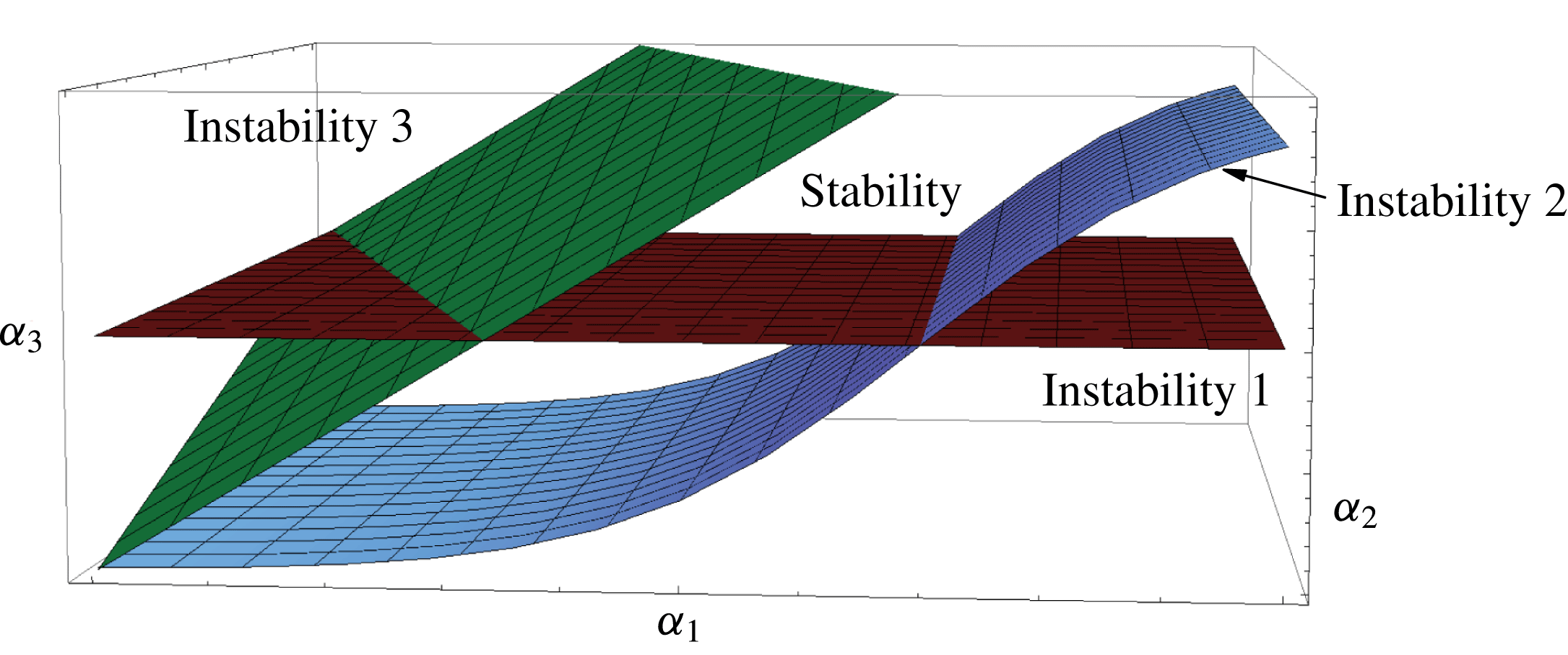
The experimental study of steady jetting stability has been frequently carried out by splitting the fluid domain into several regions and considering the mechanisms that destabilize each region separately. The steady jetting is assumed to be stable if none of those mechanisms comes into play. Each instability mechanism is represented by a surface in the parameter space characterizing the fluid configuration (figure 1). The parameter volume corresponding to stable jetting realizations is that delimited by those surfaces. The experimental data obtained to locate those surfaces are typically rationalized in terms of simple scaling analyses. In the example represented in figure 1, the stability region is bounded by three instability mechanisms in a three-dimensional parameter space.
Sketch to illustrate the way in which the steady jetting stability is frequently studied. The surfaces represent instability mechanisms in the parameter space (
 $\unicode[STIX]{x1D6FC}_{1},\unicode[STIX]{x1D6FC}_{2},\unicode[STIX]{x1D6FC}_{3}$
), frequently arising in different parts of the fluid domain. The stability region is bounded by those surfaces.

The theoretical study of steady jetting stability has been traditionally conducted also considering simple parts of the fluid domain, and applying a linear local analysis to them. An infinite cylindrical liquid jet (column) in vacuum is probably the simplest capillary system which one can think off. In this case, the study reduces to the temporal stability analysis to obtain the dispersion relationship, which allows one to calculate the continuum spectrum of eigenfrequencies characterizing the axisymmetric normal modes (Fourier components) as a function of their (real) wavenumbers (Rayleigh Reference Rayleigh1892). The decomposition of initial perturbations into the corresponding eigenmodes has proved to be useful for studying the short-term evolution of those perturbations (García & González Reference García and González2008). The above conclusions do not apply to a semi-infinite jet issuing from a nozzle. In this case, the spatial stability analysis constitutes a more realistic approach. The corresponding dispersion relation allows for the calculation of the (complex) wavenumber characterizing the perturbation evolution for a given (real) frequency (Leib & Goldstein Reference Leib and Goldstein1986). The growth rates calculated in this way are in excellent agreement with experiments (González & García Reference González and García2009).
Neither the temporal nor the spatial stability analyses of a liquid jet allow one to determine the parameter conditions for the steady jetting regime to occur when a liquid tapers from a source. For that purpose, one can conduct a spatio-temporal stability analysis (where both the wavenumber and frequency are complex numbers) to calculate the convective-to-absolute instability transition as a function of the governing parameters (Huerre & Monkewitz Reference Huerre and Monkewitz1990). It has been postulated that local convective instability throughout the whole fluid domain is sufficient to reach steady jetting. In this case, all the perturbations are convected downstream preserving both a stable liquid source and a steady filament which is long compared with its diameter. In contrast, absolute instability allows perturbations to travel upstream while growing, which is expected to cause either self-sustained oscillations or dripping. However, the link between absolute instability and these two phenomena is not clear even in relatively simple cases, where the base flow is almost uniform. For instance, Yakubenko (Reference Yakubenko1997) has showed that inclined jets can suffer from self-sustained oscillations even if they are convectively unstable throughout the whole fluid domain. The Weber number for the convective-to-absolute instability transition significantly differs from that corresponding to the steady jetting instability in both plane liquid sheets (de Luca Reference de Luca1999) and round jets (Dizes Reference Dizes1997).
The main limitation of the spatio-temporal stability analysis is its local character, i.e. it is valid as long as the base flow explored by the perturbations is quasi-parallel and quasi-homogeneous in the streamwise direction. This approach has been successfully applied to slowly spatially developing (weakly non-parallel) base flows (Chomaz Reference Chomaz2005; Tammisola et al. Reference Tammisola, Sasaki, Lundell, Matsubara and Soderberg2011). However, there are many applications where the hydrodynamic length characterizing the base flow is of the order of, or even much smaller than, that of the dominant perturbation, which invalidates the local approximation. In these cases, an accurate stability analysis requires the calculation of the global modes, which sheds new light in the physical mechanisms at play.
Global modes are patterns of motion depending in an inhomogeneous way on two or three spatial directions, and in which the entire system moves harmonically with the same (complex) frequency and a fixed phase relation (Theofilis Reference Theofilis2011). They are calculated as the eigenfunctions of the linearized Navier–Stokes operator as applied to a given configuration (base flow). If the spectrum of eigenvalues is in the stable complex half-plane, the base flow is linearly and asymptotically stable, which means that any initial small-amplitude perturbation will decay exponentially on time for
 $t\rightarrow \infty$
(as long as the linear approximation applies). Global instability is frequently linked to the convective-to-absolute instability transition, and is also assumed to cause either self-sustained oscillations or dripping. Tammisola, Lundell & Soderberg (Reference Tammisola, Lundell and Soderberg2012) have studied the effect of surface tension on the global stability of coflow jets and wakes at a moderate Reynolds number. Sauter & Buggisch (Reference Sauter and Buggisch2005) and Gordillo et al. (Reference Gordillo, Sevilla and Campo-Cortés2014) have examined the global stability of jets stretched by the action of gravity and a coflowing stream, respectively.
Linear asymptotic global stability does not necessarily imply linear stability. If the linearized Navier–Stokes operator is normal, then the perturbation energy decreases monotonically not only in the asymptotic regime but also during the system’s short-term response. In contrast, if this last condition does not apply, there can be a transient growth of the perturbation energy before the asymptotic exponential regime is reached (Chomaz Reference Chomaz2005; Schmid Reference Schmid2007). The short-term, non-exponential growth of small-amplitude perturbations can be responsible for the instability of asymptotically stable systems. In fact, convective instabilities commonly arising in problems with inflow and outflow conditions are not typically dominated by the long-term modal behaviour. For instance, asymptotically stable gravitational jets eventually break up due to the growth of non-normal modes (de Luca, Costa & Caramiello Reference de Luca, Costa and Caramiello2002). Therefore, a base flow is stable according to linear asymptotic global stability only if (i) all the linear eigenmodes are stable, and (ii) the linearized Navier–Stokes operator associated with that flow is normal. If this last condition does not verify, more sophisticated approaches have to be taken to accurately capture the short-time dynamics, which may be more relevant to the overall flow physics.
Axisymmetric gaseous flow focusing (Gañán-Calvo Reference Gañán-Calvo1998) has become a very popular technique to produce droplets in the steady jetting mode with diameters ranging from the submillimetre to the micrometre scale (Forbes & Sisco Reference Forbes and Sisco2014; Si et al. Reference Si, Feng, Luo and Xu2014; Trebbin et al. Reference Trebbin, Kruger, DePonte, Roth, Chapman and Forster2014). In this technique, a high-speed gas stream transfers energy to the liquid accumulated in a meniscus hanging on a feeding capillary through the collaborative action of both hydrostatic pressure and viscous shear forces. Flow focusing is attractive because produces jets much thinner than the discharge orifice, making use of purely hydrodynamic means, with no restrictions on the liquid properties.
The minimum droplet diameter in flow focusing is fundamentally determined by the axisymmetric instability arising when the injected liquid flow rate decreases below a certain threshold (Si et al. Reference Si, Li, Yin and Yin2009; Vega et al. Reference Vega, Montanero, Herrada and Gañán-Calvo2010; Montanero et al. Reference Montanero, Rebollo-Muñoz, Herrada and Gañán-Calvo2011). This instability limit has been analysed in terms of both the convective-to-absolute instability transition in the emitted jet for low gas speeds, and the breakdown of the balance between viscosity, surface tension and inertia in the liquid meniscus for sufficiently high gas velocities. The understanding of these two instability mechanisms has allowed us to rationalize the experimental results obtained both in the low- (Vega et al. Reference Vega, Montanero, Herrada and Gañán-Calvo2010) and high-viscosity (Montanero et al. Reference Montanero, Rebollo-Muñoz, Herrada and Gañán-Calvo2011) limits. However, there is not as yet a comprehensive study to describe the minimum flow rate instability on a rigorous basis.
In this paper, we will conduct a linear global stability analysis of the base flow arising when a liquid meniscus is focused by a high-speed gaseous stream crossing a converging–diverging nozzle (DePonte et al. Reference DePonte, Weierstall, Schmidt, Warner, Starodub, Spence and Doak2008; Acero et al. Reference Acero, Ferrera, Montanero and Gañán-Calvo2012). We will calculate the axisymmetric eigenmodes, and determine the system’s global stability limit as the parameter conditions for which the dominant mode becomes unstable. The comparison with experimental results will show that this analysis significantly underestimates the minimum flow rate for small enough gas speeds, which reveals the inability of the asymptotic stability theory to describing the short-term dynamics. This conclusion will be confirmed by direct numerical simulations of both the linearized and nonlinear Navier–Stokes equations, which will show how perturbations introduced into globally stable base flows can grow over time. We will not consider the whipping instability because: (i) it strongly depends on the shape of the nozzle, which hinders the comparison between the numerical and experimental results; and (ii) the computing time for direct numerical simulations increases very significantly.
2 Axisymmetric gaseous flow focusing
2.1 Formulation of the problem
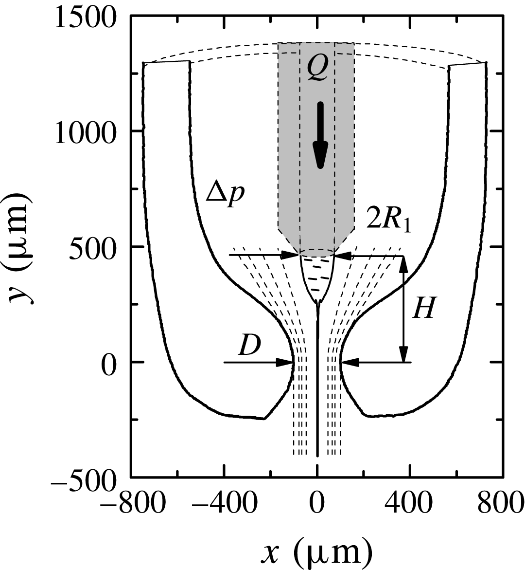
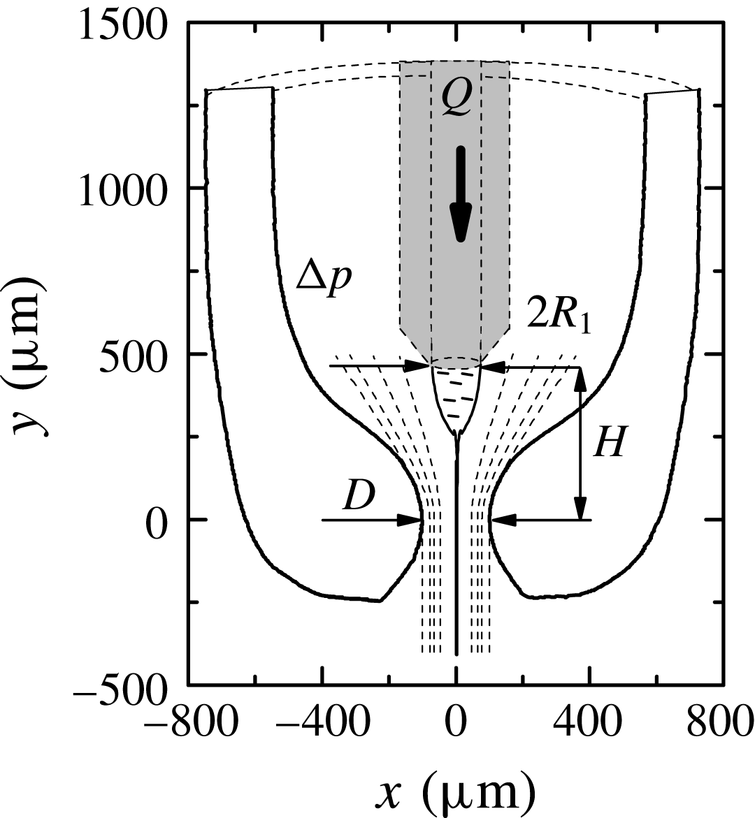
Figure 2 shows the axisymmetric gaseous flow focusing configuration considered in this paper. A liquid of density
 $\unicode[STIX]{x1D70C}_{\ell }$
and viscosity
 $\unicode[STIX]{x1D707}_{\ell }$
is injected through a feeding capillary of radius
 $R_{1}$
at a constant flow rate
 $Q$
. The feeding capillary is located inside a converging–diverging nozzle with an orifice of diameter
 $D$
. The distance between the capillary end and the nozzle neck is
 $H$
. A gas stream of density
 $\unicode[STIX]{x1D70C}_{g}$
and viscosity
 $\unicode[STIX]{x1D707}_{g}$
flows through the nozzle driven by the applied pressure drop
 $\unicode[STIX]{x0394}p$
. An axisymmetric meniscus hangs on the edge of the capillary end due to the action of the surface tension
 $\unicode[STIX]{x1D70E}$
. In the steady jetting regime, a liquid microjet tapers from the meniscus tip, and crosses the nozzle coflowing with the outer gas stream.
Axisymmetric gaseous flow focusing. The geometrical configuration corresponds to that used in the experiments by Acero et al. (Reference Acero, Ferrera, Montanero and Gañán-Calvo2012). The values of the main parameters are
 $R_{1}\simeq 75~\unicode[STIX]{x03BC}\text{m}$
,
 $D\simeq 200~\unicode[STIX]{x03BC}\text{m}$
and
 $H\simeq 440~\unicode[STIX]{x03BC}\text{m}$
.
The interfacial (capillary) sink of energy typically plays a secondary role as compared to the jet’s kinetic energy (Gañán-Calvo Reference Gañán-Calvo1998). For this reason, the jet’s radius downstream,
 $R_{j}$
, essentially depends on the liquid density
 $\unicode[STIX]{x1D70C}_{\ell }$
and viscosity
 $\unicode[STIX]{x1D707}_{\ell }$
, as well as on the control parameters
 $Q$
and
 $\unicode[STIX]{x0394}p$
. If one also neglects the viscous dissipation of energy, the conservation of this quantity yields (Gañán-Calvo Reference Gañán-Calvo1998)
 $$\begin{eqnarray}R_{j}=R_{FF}\equiv \left(\frac{\unicode[STIX]{x1D70C}_{\ell }Q^{2}}{2\unicode[STIX]{x03C0}^{2}\unicode[STIX]{x0394}p}\right)^{1/4}.\end{eqnarray}$$
This characteristic length allows one to define the Reynolds and Weber numbers
 $$\begin{eqnarray}Re_{FF}=\frac{\unicode[STIX]{x1D70C}_{\ell }V_{FF}R_{FF}}{\unicode[STIX]{x1D707}_{\ell }}\quad \text{and}\quad We_{FF}=\frac{\unicode[STIX]{x1D70C}_{\ell }V_{FF}^{2}R_{FF}}{\unicode[STIX]{x1D70E}},\end{eqnarray}$$
where
 $V_{FF}\equiv Q/(\unicode[STIX]{x03C0}R_{FF}^{2})$
is the jet’s mean velocity calculated from
 $R_{FF}$
. The density and viscosity ratios,
 $\unicode[STIX]{x1D70C}=\unicode[STIX]{x1D70C}_{g}/\unicode[STIX]{x1D70C}_{\ell }$
and
 $\unicode[STIX]{x1D707}=\unicode[STIX]{x1D707}_{g}/\unicode[STIX]{x1D707}_{\ell }$
, take very small values in gaseous flow focusing, and thus their influence on the steady jetting stability can be neglected. For a fixed geometrical configuration, the three governing (dimensionless) parameters are
 $Re_{FF}$
,
 $We_{FF}$
and the Ohnesorge number
 $C=\unicode[STIX]{x1D707}_{\ell }(\unicode[STIX]{x1D70C}_{\ell }\unicode[STIX]{x1D70E}R_{1})^{-1/2}$
.
2.2 Previous experimental results
Most of previous studies (Gañán-Calvo Reference Gañán-Calvo1998; Si et al.
Reference Si, Li, Yin and Yin2009; Vega et al.
Reference Vega, Montanero, Herrada and Gañán-Calvo2010; Acero et al.
Reference Acero, Ferrera, Montanero and Gañán-Calvo2012) have examined the original flow focusing configuration (Gañán-Calvo Reference Gañán-Calvo1998) where the nozzle is replaced by a plate with an orifice. In these studies, the analysis has been simplified by examining the stability of the liquid source (meniscus) and the emitted jet separately (as suggested by the clear separation furnished by the plate): the steady jetting regime is assumed to be stable if and only if these two subdomains are stable. The liquid flow rate leading to the meniscus instability has been estimated through simple scaling analyses in both the inviscid (Vega et al.
Reference Vega, Montanero, Herrada and Gañán-Calvo2010) and viscous limits (Montanero et al.
Reference Montanero, Rebollo-Muñoz, Herrada and Gañán-Calvo2011). The jet’s behaviour has been described in terms of the spatio-temporal stability analysis for a uniform base flow (Leib & Goldstein Reference Leib and Goldstein1986), which allows one to determine whether the jet is either convectively or absolutely unstable. Finally, for high enough liquid viscosities, the system runs into the surface tension barrier at the jet inception,
 $We_{FF}\simeq 1$
(Eggers & Villermaux Reference Eggers and Villermaux2008), before the jet becomes absolutely unstable. Therefore, steady jetting gives rise to dripping if one of the above three instability limits is reached. Experimental results have shown that the first limit arises in the first place for large enough applied pressure drops (gas speeds) (Montanero et al.
Reference Montanero, Rebollo-Muñoz, Herrada and Gañán-Calvo2011), while either the second or the third condition determines the steady jetting stability for sufficiently low values of
 $\unicode[STIX]{x0394}p$
(Si et al.
Reference Si, Li, Yin and Yin2009; Vega et al.
Reference Vega, Montanero, Herrada and Gañán-Calvo2010).
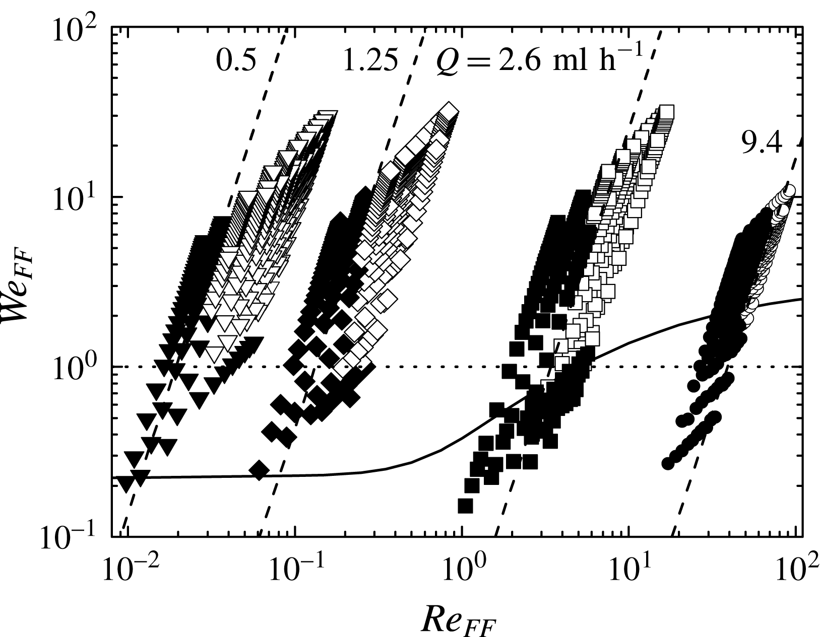
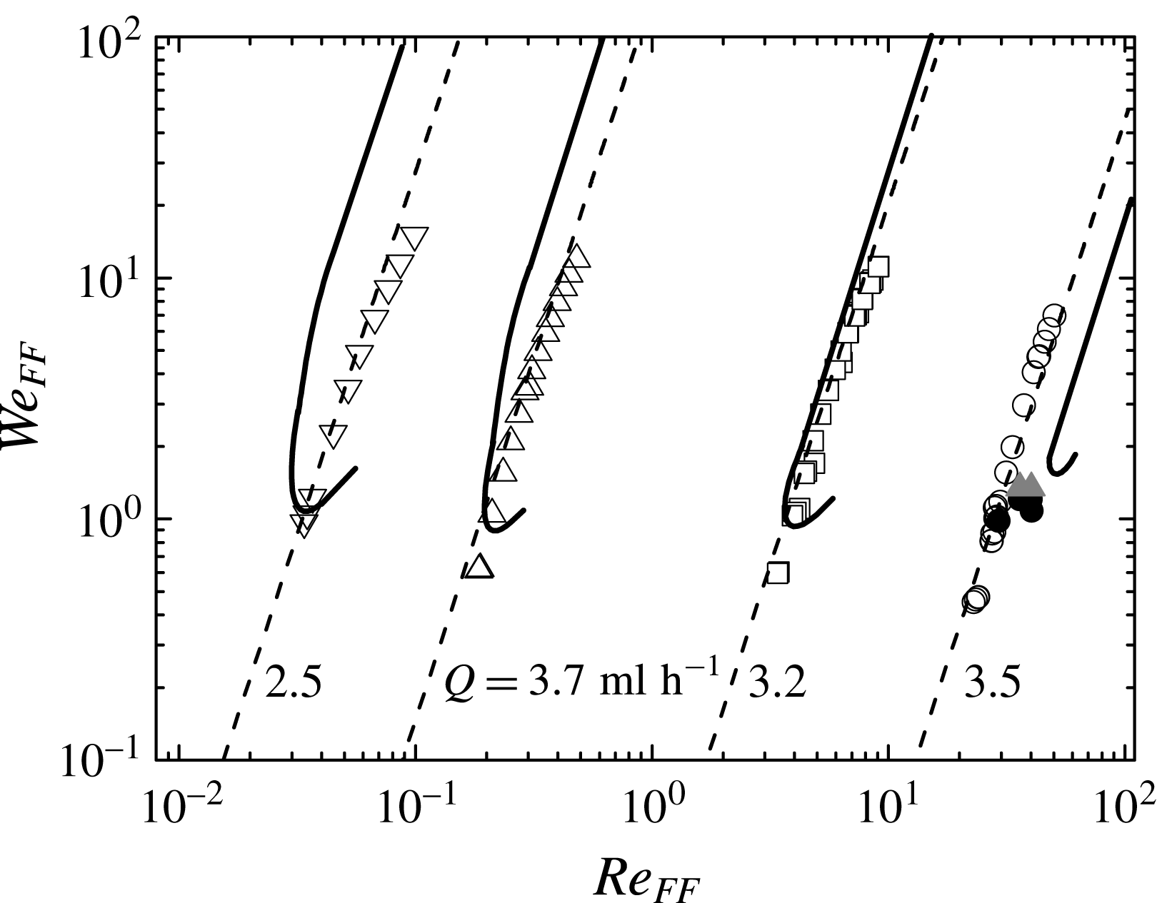
Stability map for the flow focusing configuration shown in figure 2. The circles, squares, diamonds and triangles correspond to water, 5-cSt silicone oil, 100-cSt silicone oil and 500-cSt silicone oil, respectively. The white and black symbols correspond to the steady jetting and dripping regimes, respectively. The solid line is Leib and Goldstein’s prediction for the convective/absolute instability transition in a capillary jet (Leib & Goldstein Reference Leib and Goldstein1986). The dashed lines are the curves
 $Q=\text{const}$
. The labels indicate the corresponding flow rates as obtained from the jetting-to-dripping transition for
 $\unicode[STIX]{x0394}p=250$
mbar. The dotted line is the boundary
 $We_{FF}=1$
.

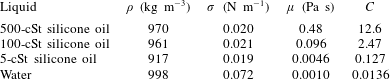
Experiments were conducted by Acero et al. (Reference Acero, Ferrera, Montanero and Gañán-Calvo2012) to examine the stability of the steady jetting regime when focusing a liquid stream in a converging nozzle. For this purpose, the steady jetting was established for a sufficiently high liquid flow rate, and then the value of this quantity was progressively decreased while keeping the applied pressure drop constant. Figure 3 shows the projection of the experimental results onto the parameter plane defined by the Reynolds and Weber numbers (2.2) for different Ohnesorge numbers. The properties of the working liquids and the corresponding values of the Ohnesorge number are displayed in table 1. The steady jetting realizations also include those where the jet bends due to the whipping instability (not considered in this work). The jetting mode is limited by the existence of a minimum flow rate for large enough applied pressure drops (Vega et al.
Reference Vega, Montanero, Herrada and Gañán-Calvo2010; Acero et al.
Reference Acero, Ferrera, Montanero and Gañán-Calvo2012). When this parameter takes small values, the jet’s behaviour depends on the liquid viscosity: the convective-to-absolute instability transition becomes dominant for low and moderate viscosities (water and 5-cSt silicone oil) (Vega et al.
Reference Vega, Montanero, Herrada and Gañán-Calvo2010), while the instability barrier
 $We_{FF}\simeq 1$
is reached in the high-viscosity cases (100-cSt and 500-cSt silicone oils) before the jet becomes absolutely unstable (Acero et al.
Reference Acero, Ferrera, Montanero and Gañán-Calvo2012).
Properties of the focused liquids at
 $20\,^{\circ }\text{C}$
.

As can be seen, the stability analysis of axisymmetric flow focusing is a compendium of several rules which must be applied in a different way depending on the properties of the focused liquids. In particular, the local stability analysis of the emitted jet does not predict the existence of a minimum flow rate for large applied pressure drops, which is the most relevant stability limit at the technological level. Therefore, a comprehensive and more rigorous stability study of the present fluid configuration is desirable. This study demands the calculation of the linear global modes.
3 Governing equations
In this section, all the variables are made dimensionless with the capillary radius
 $R_{1}$
, the liquid density
 $\unicode[STIX]{x1D70C}_{\ell }$
and the surface tension
 $\unicode[STIX]{x1D70E}$
, which yield the characteristic time and velocity scales
 $t_{c}=(\unicode[STIX]{x1D70C}_{\ell }R_{1}^{3}/\unicode[STIX]{x1D70E})^{1/2}$
and
 $v_{c}=R_{1}/t_{c}$
, respectively. The dimensionless, axisymmetric, incompressible Navier–Stokes equations for the velocity
 $\boldsymbol{v}^{(j)}(r,z;t)$
and pressure
 $p^{(j)}(r,z;t)$
fields are
 $$\begin{eqnarray}\displaystyle & \displaystyle [ru^{(j)}]_{r}+rw_{z}^{(j)}=0, & \displaystyle\end{eqnarray}$$
 $$\begin{eqnarray}\displaystyle & \displaystyle \unicode[STIX]{x1D70C}^{\unicode[STIX]{x1D6FF}_{jg}}(u_{t}^{(j)}+u^{(j)}u_{r}^{(j)}+w^{(j)}u_{z}^{(j)})=-p_{r}^{(j)}+\unicode[STIX]{x1D707}^{\unicode[STIX]{x1D6FF}_{jg}}C[u_{rr}^{(j)}+(u^{(j)}/r)_{r}+u_{zz}^{(j)}], & \displaystyle\end{eqnarray}$$
 $$\begin{eqnarray}\displaystyle & \displaystyle \unicode[STIX]{x1D70C}^{\unicode[STIX]{x1D6FF}_{jg}}(w_{t}^{(j)}+u^{(j)}w_{r}^{(j)}+w^{(j)}w_{z}^{(j)})=-p_{z}^{(j)}+\unicode[STIX]{x1D707}^{\unicode[STIX]{x1D6FF}_{jg}}C[w_{rr}^{(j)}+w_{r}^{(j)}/r+w_{zz}^{(j)}], & \displaystyle\end{eqnarray}$$
where
 $t$
is the time,
 $r$
(
 $z$
) is the radial (axial) coordinate,
 $u^{(j)}$
(
 $w^{(j)}$
) is the radial (axial) velocity component and
 $\unicode[STIX]{x1D6FF}_{ij}$
is the Kronecker delta. In the above equations and henceforth, the superscripts
 $j=\ell$
and
 $g$
refer to the liquid and gas phases, respectively, while the subscripts
 $t$
,
 $r$
and
 $z$
denote the partial derivatives with respect to the corresponding variables. The action of the gravitational field has been neglected due to the smallness of the fluid configuration.
Taking into account the kinematic compatibility and equilibrium of tangential and normal stresses at the interface
 $r=F(z,t)$
, one obtains the following equations:
 $$\begin{eqnarray}\displaystyle & \displaystyle F_{t}+F_{z}w^{(\ell )}-u^{(\ell )}=F_{t}+F_{z}w^{(g)}-u^{(g)}=0, & \displaystyle\end{eqnarray}$$
 $$\begin{eqnarray}\displaystyle & \displaystyle (1-F_{z}^{2})(w_{r}^{(\ell )}+u_{z}^{(\ell )})+2F_{z}(u_{r}^{(\ell )}-w_{z}^{(\ell )})=\unicode[STIX]{x1D707}[(1-F_{z}^{2})(w_{r}^{(g)}+u_{z}^{(g)})+2F_{z}(u_{r}^{(g)}-w_{z}^{(g)})], & \displaystyle \nonumber\\ \displaystyle & & \displaystyle\end{eqnarray}$$
 $$\begin{eqnarray}\displaystyle & & \displaystyle p^{(\ell )}+\frac{FF_{zz}-1-F_{z}^{2}}{F(1+F_{z}^{2})^{3/2}}-\frac{2C[u_{r}^{(\ell )}-F_{z}(w_{r}^{(\ell )}+u_{z}^{(\ell )})+F_{z}^{2}w_{z}^{(\ell )}]}{1+F_{z}^{2}}\nonumber\\ \displaystyle & & \displaystyle \qquad =p^{(g)}-\frac{2\unicode[STIX]{x1D707}C[u_{r}^{(g)}-F_{z}(w_{r}^{(g)}+u_{z}^{(g)})+F_{z}^{2}w_{z}^{(g)}]}{1+F_{z}^{2}}.\end{eqnarray}$$
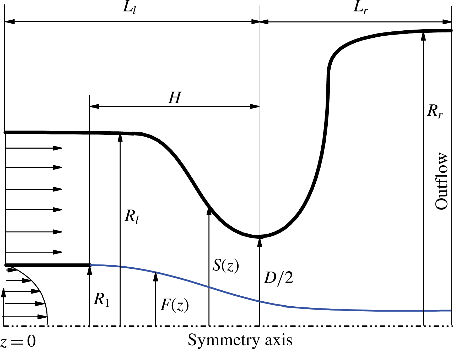
The Navier–Stokes equations are integrated in the numerical domain sketched in figure 4. The (dimensionless) shape
 $S(z)$
of the nozzle is given by the function
 $$\begin{eqnarray}S(z)=\left\{\begin{array}{@{}ll@{}}R_{ml}-a_{l}\tanh [\unicode[STIX]{x1D6FC}_{l}(z-z_{ml})]\quad & \text{for}~0\leqslant z\leqslant L_{l}\\ R_{mr}+a_{r}\tanh [\unicode[STIX]{x1D6FC}_{r}(z-z_{mr})]\quad & \text{for}~L_{l}<z\leqslant L_{l}+L_{r},\end{array}\right.\end{eqnarray}$$
where
 $R_{ml,r}=(R_{l,r}+D/2)/2$
and
 $a_{l,r}=(R_{l,r}-D/2)/2$
. The shape of the converging part of the nozzle is given by the parameters
 $R_{l}$
,
 $D$
and
 $\unicode[STIX]{x1D6FC}_{l}$
, while its position in our coordinate system and length are determined from
 $z_{ml}$
and
 $L_{l}$
, respectively. Analogously, the shape of the diverging part of the nozzle is defined by the parameters
 $R_{r}$
,
 $D$
and
 $\unicode[STIX]{x1D6FC}_{r}$
, while its length is
 $L_{r}$
. The mid-point axial position of the diverging part,
 $z_{mr}$
, is calculated from the continuity condition of
 $S(z)$
at
 $z=L_{l}$
. Finally, the parameter
 $H$
characterizes the axial position of the feeding capillary end in the nozzle. In our simulations,
 $R_{l}=2.67$
,
 $R_{r}=5.33$
,
 $D=2.59$
,
 $\unicode[STIX]{x1D6FC}_{l}=\unicode[STIX]{x1D6FC}_{r}=1$
,
 $z_{ml}=6.93$
,
 $L_{l}=L_{r}=10$
and
 $H=5.87$
. The main geometrical parameters
 $R_{1}$
,
 $D$
and
 $H$
approximately coincide with those of the experiments of Acero et al. (Reference Acero, Ferrera, Montanero and Gañán-Calvo2012) (figure 2).
Sketch of the computational domain.

At the inlet section
 $z=0$
, we impose a uniform velocity profile in the gaseous stream, and the Hagen–Poiseuille velocity distribution
 $u^{(\ell )}=0$
and
 $w^{(\ell )}=2v_{e}(1-r^{2})$
(
 $v_{e}=Q/(\unicode[STIX]{x03C0}R_{1}^{2}v_{c})$
) in the liquid domain. The gas inlet velocity is adjusted so that the pressure drop
 $\unicode[STIX]{x0394}p$
between the inlet and outlet sections of the numerical domain corresponds to that of the experiments. The no-slip boundary condition is imposed at the solid walls. The free-surface shape is obtained as part of the solution by considering the anchorage condition
 $F=1$
of the triple contact line at the edge of the feeding capillary. We prescribe the standard regularity conditions
 $u^{(\ell )}=w_{r}^{(\ell )}=0$
at the symmetry axis, and the outflow conditions
 $u_{z}^{(j)}=w_{z}^{(j)}=F_{z}=0$
at the right-hand end
 $z=L_{l}+L_{r}$
of the computational domain. We verified that the results are not significantly affected by this last condition by comparing the stability limits for different values of
 $L_{r}$
. Specifically, we increased
 $L_{r}$
by a 50 % and the minimum flow rate differed in less than 1 % in all the cases analysed.
The fluid domain is mapped onto a fixed numerical domain through a coordinate transformation. The hydrodynamic equations are discretized in the radial direction with 11 and 35 Chebyshev spectral collocation points in the liquid and gas domains, respectively. In the axial direction, we use fourth-order finite differences with 1001 equally spaced points. We conducted simulations for different mesh sizes to ensure that the results did not depend on that choice. To calculate the linear global modes, one assumes the temporal dependence
 $$\begin{eqnarray}U(r,z;t)=U_{0}(r,z)+\unicode[STIX]{x1D700}\unicode[STIX]{x1D6FF}U(r,z)\,\text{e}^{-\text{i}\unicode[STIX]{x1D714}t}\quad (\unicode[STIX]{x1D700}\ll 1).\end{eqnarray}$$
Here,
 $U(r,z;t)$
represents any hydrodynamic quantity,
 $U_{0}(r,z)$
and
 $\unicode[STIX]{x1D6FF}U(r,z)$
stand for the base (steady) solution and the spatial dependence of the eigenmode, respectively, while
 $\unicode[STIX]{x1D714}=\unicode[STIX]{x1D714}_{r}+\text{i}\unicode[STIX]{x1D714}_{i}$
is the eigenfrequency. Both the eigenfrequencies
 $\unicode[STIX]{x1D714}$
and the corresponding eigenmodes
 $\unicode[STIX]{x1D6FF}U$
are calculated as a function of the governing parameters. The dominant eigenmode is that with the largest growth factor
 $\unicode[STIX]{x1D714}_{i}$
. If that growth factor is positive, the base flow is asymptotically unstable (Theofilis Reference Theofilis2011).
In both the linearized and nonlinear direct numerical simulations, implicit time advancement is performed using second-order backward finite differences. At each time step, the resulting set of algebraic equations is solved by inverting the coefficient matrix and by applying the iterative Newton–Raphson technique in the linear and nonlinear cases, respectively. Details of the numerical procedure can be found elsewhere (Herrada & Montanero Reference Herrada and Montanero2016), where we explain how the numerical procedures for solving the eigenvalue and time-dependent problems are essentially the same. One of the main characteristics of these procedures is that the elements of the Jacobian of the discretized system of equations are computed via standard symbolic software at the outset, before running the simulation. In the nonlinear direct numerical simulations, these functions are evaluated numerically over the Newton–Raphson iterations to find the solution at each time step, which reduces considerably the required CPU time. The initial guess for the iterations at each time step is the solution at the previous instant.
4 Results
4.1 Linear global modes
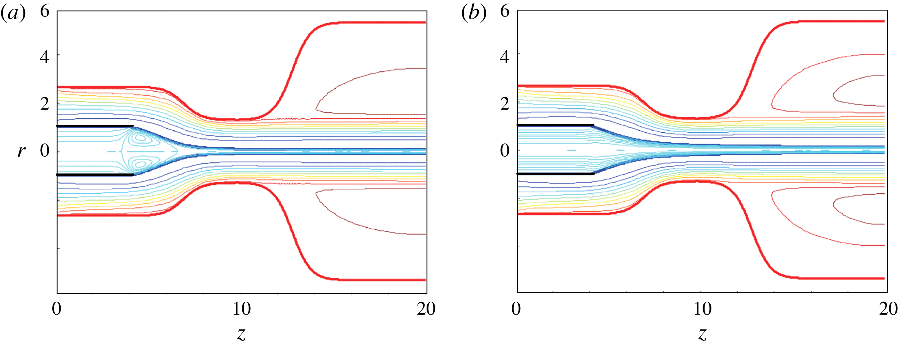
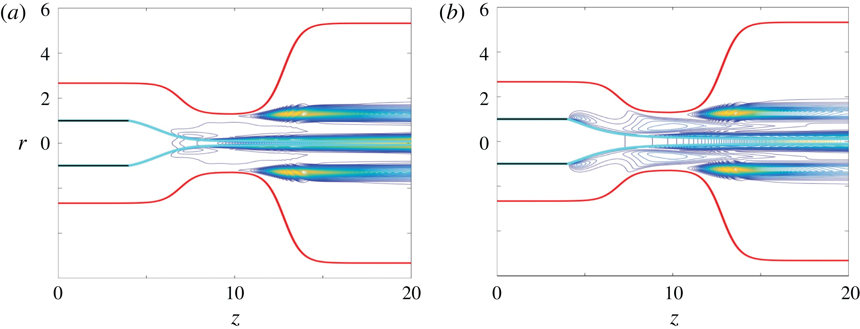
Figure 5 shows two stable base flows calculated for the lowest and highest Ohnesorge numbers considered in this work. In the low Ohnesorge number case, the viscous shear stress exerted by the high-speed gas stream over the free surface accelerates the liquid there, and drags it towards the meniscus tip. The pressure increases at the stagnation point located right in front of the emitted jet, which pushes the liquid backwards across the meniscus. The resulting recirculation cell occupies the entire meniscus and enters the feeding capillary. In the high Ohnesorge number case, the gas current does not form the recirculation cell due to the strong viscous stresses arising in the liquid meniscus. Those stresses ‘arrange’ the streamlines and ‘direct’ the flow in the meniscus tip. The resulting flow pattern becomes similar to that appearing in liquid–liquid coflowing configurations.
Base flow for
 $Re_{FF}=34.3$
,
 $We_{FF}=2.03$
and
 $C=0.0136$
(a), and for
 $Re_{FF}=0.045$
,
 $We_{FF}=2.27$
and
 $C=12.6$
(b).

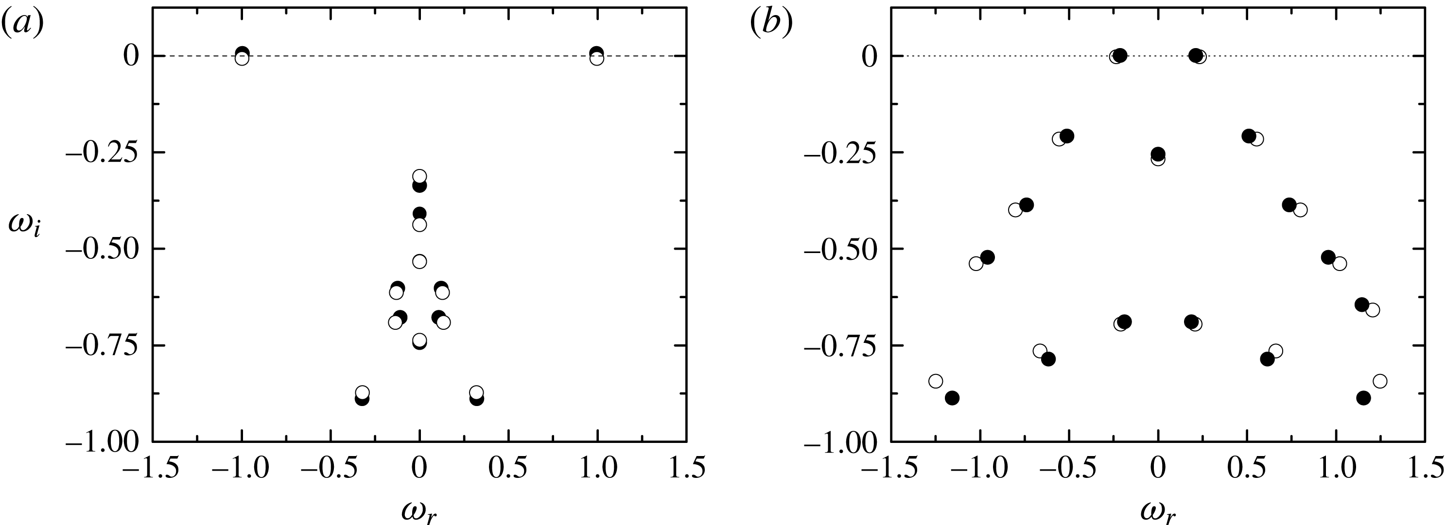
Figure 6 shows the spectrum of eigenvalues
 $\unicode[STIX]{x1D714}=\unicode[STIX]{x1D714}_{r}+\text{i}\unicode[STIX]{x1D714}_{i}$
with oscillation frequencies
 $\unicode[STIX]{x1D714}_{r}$
around that of the dominant mode. The open symbols are the eigenvalues characterizing the linear global modes of the stable base flows in figure 5, while the solid symbols correspond to those obtained when the liquid flow rate is slightly decreased while keeping the applied pressure drop constant until those flows become asymptotically unstable. The point representing the dominant global mode slightly moves up, and crosses the complex plane imaginary axis causing asymptotic instability. The frequency of this mode is around unity for the low-viscosity liquid. This means that the flow focusing steady regime becomes asymptotically unstable due to the unbounded growth of self-excited oscillations characterized by a frequency that approximately equals the inverse of the capillary time. The frequency of the dominant mode considerably decreases as viscosity increases, while the opposite occurs to the subdominant ones.
(a) Eigenvalues for
 $Re_{FF}=33.3$
,
 $We_{FF}=2.03$
and
 $C=0.0136$
(open symbols), and for
 $Re_{FF}=33.6$
,
 $We_{FF}=1.98$
and
 $C=0.0136$
(solid symbols). (b) Eigenvalues for
 $Re_{FF}=0.0450$
,
 $We_{FF}=2.27$
and
 $C=12.6$
(open symbols), and for
 $Re_{FF}=0.0421$
,
 $We_{FF}=2.12$
and
 $C=12.6$
(solid symbols).

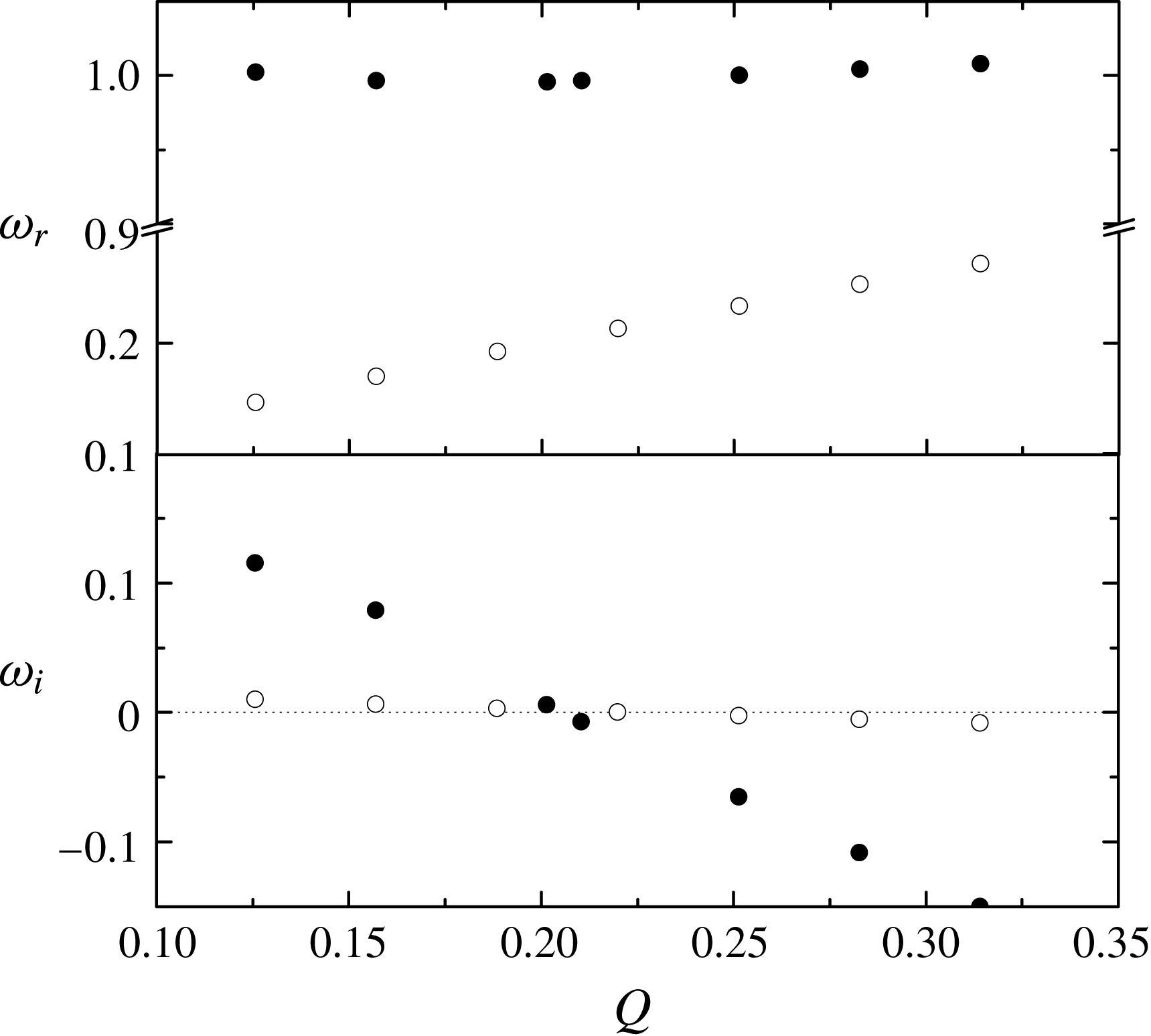
Figure 7 shows the evolution of the dominant eigenvalue as the liquid flow rate decreases for a constant applied pressure drop. This figure illustrates what happens in a typical flow focusing experiment, when the stability limit is determined starting from a stable configuration for a sufficiently large flow rate, and then this quantity is progressively decreased while keeping the applied pressure constant (Acero et al.
Reference Acero, Ferrera, Montanero and Gañán-Calvo2012). The oscillation frequency
 $\unicode[STIX]{x1D714}_{r}$
of the dominant mode is practically independent of the liquid flow rate in the low-viscosity case, while it significantly decreases as
 $Q$
decreases for the viscous liquid. The growth rate exhibits a quasi-linear dependence with respect to the liquid flow rate in both the low- and high-viscosity cases. The slope of the curve
 $\unicode[STIX]{x1D714}_{i}(Q)$
for the viscous liquid is much smaller than in the low-viscosity case, which suggests that the minimum flow rate is more sensitive to variations of the rest of governing parameters in the former case. The minimum flow rate is approximately
 $0.2(\unicode[STIX]{x1D70E}R_{1}^{3}/\unicode[STIX]{x1D70C})^{1/2}$
for both water and 500-cSt silicone oil. Because the water surface tension is much larger than that of 500-cSt silicone oil, the above result implies that the minimum flow rate is considerably smaller in the latter case, in agreement with previous experimental observations (Acero et al.
Reference Acero, Ferrera, Montanero and Gañán-Calvo2012).
Oscillation frequency
 $\unicode[STIX]{x1D714}_{r}$
and growth factor
 $\unicode[STIX]{x1D714}_{i}$
as a function of the liquid flow rate
 $Q$
for
 $\unicode[STIX]{x0394}p=7.78$
. The solid and open symbols correspond to
 $C=0.0136$
and 12.6, respectively.

The stability limits corresponding to the jetting-to-dripping transition in figure 3 are compared with the corresponding predictions obtained from the asymptotic global stability analysis in figure 8. There is remarkable agreement between the experimental and theoretical results for 5-cSt silicone oil. The linear stability analysis satisfactorily captures the influence of viscosity in all the cases. The theoretical predictions for water systematically underestimate the critical flow rate for Weber numbers larger than unity (large applied pressure drops), which leads to a stable parameter region bigger than that observed in the experiments. This discrepancy can be explained in terms of the finite-amplitude perturbations that inevitably appear in experiments, which can destabilize configurations stable under infinitesimal disturbances. The pressure waves driven by the syringe pump used to inject the liquid constitutes an example of such perturbations (Korczyk et al. Reference Korczyk, Cybulski, Makulskaa and Garstecki2011).
Stability map for the flow focusing configuration shown in figure 2. From right to left, the solid lines approximately correspond to the experimental jetting-to-dripping transitions shown in figure 3 for
 $C=0.0136$
(water), 0.127 (5-cSt silicone oil), 2.47 (100-cSt silicone oil) and 12.6 (500-cSt silicone oil), respectively. The open symbols are the corresponding transitions from asymptotically stable-to-unstable base flows. The figure shows the minimum flow rates estimated from these theoretical predictions. The solid triangles and circles are stable and unstable direct numerical simulations for water, respectively.

The theoretical predictions for 100-cSt and 500-cSt silicone oil systematically overestimate the minimum flow rate for Weber numbers larger than unity. This means that steady jetting realizations were observed in the experiments even for asymptotically unstable configurations. This discrepancy cannot be attributed to potentially stabilizing effects of nonlinear terms, which would yield self-sustained oscillations not observed in the experiments. However, it might be caused by the possibly stabilizing role played by the jet/meniscus bending taking place in the experiments for high viscosities (Acero et al.
Reference Acero, Ferrera, Montanero and Gañán-Calvo2012), which is not considered in our axisymmetric theoretical analysis. In fact, the minimum flow rates estimated from the theoretical predictions (figure 8) are consistent with the trends observed in figure 8 of Montanero et al. (Reference Montanero, Rebollo-Muñoz, Herrada and Gañán-Calvo2011) for large
 $H$
in the plate–orifice configuration, where whipping does not occur.
Another plausible explanation for the deviation between the asymptotic global stability analysis and the experiments may be found in the differences between the numerical and experimental geometries. On one side, the nozzle inner shape was modelled in the simulations by the function (3.7) to simplify the numerical calculations. On the other side, the experiments were conducted for a large ratio
 $H/D$
(close to its maximum possible value), and therefore small variations of the capillary position
 $H$
must considerably influence the critical flow rate, according to the experimental data of Montanero et al. (Reference Montanero, Rebollo-Muñoz, Herrada and Gañán-Calvo2011) for the plate–orifice configuration. These geometrical deviations are expected to affect the minimum flow rate to a greater extent for high viscosities because of the large sensitivity of that threshold to small variations of the rest of parameters in that case (figure 7). Confirming the validity of this explanation would require a systematic parameter study that is beyond the scope of the present work.
The asymptotic stability limit curves do not have the ‘elbow’ observed in the experiments for Weber numbers around unity. In the next subsection, we will explain this discrepancy in terms of a convective instability resulting from the superposition at short times of asymptotically stable global modes. For this purpose, the Navier–Stokes equations will be integrated over time to monitor the evolution of small perturbations introduced into the liquid meniscus. It must be noted that previous studies (Si et al. Reference Si, Li, Yin and Yin2009; Montanero et al. Reference Montanero, Rebollo-Muñoz, Herrada and Gañán-Calvo2011) have already recognized that the nature of this instability is different from that arising for large pressure drops (Weber numbers). In fact, they have described the phenomenon in terms of the convective-to-absolute instability transition (Huerre & Monkewitz Reference Huerre and Monkewitz1990) taking place in an infinite cylindrical jet.
In order to gain insight into the physical mechanisms responsible for the asymptotic global instability, we consider the kinetic energy
 $e\equiv p+1/2\,\unicode[STIX]{x1D70C}^{\unicode[STIX]{x1D6FF}_{jg}}\,(|u^{(j)}|^{2}+|w^{(j)}|^{2})$
associated with the eigenmode. Figure 9 shows the isolines of this quantity for the modes causing the instability of the base flows in figure 5. The scalar fields
 $e(r,z)$
in the liquid and gas domains have been normalized with their corresponding maximum values. The maximum values in the liquid domain are approximately 132 and 37 times as those of the gas stream for the low- and high-viscosity cases, respectively. This indicates that the physical origin of the instability must be located in the liquid domain, as assumed in previous studies (Si et al.
Reference Si, Li, Yin and Yin2009; Montanero et al.
Reference Montanero, Rebollo-Muñoz, Herrada and Gañán-Calvo2011; Acero et al.
Reference Acero, Ferrera, Montanero and Gañán-Calvo2012). The perturbation energy in the liquid domain increases monotonously along the streamwise direction. The perturbation energy of the gas increases both next to the jet’s free surface and in the shear layers between the gas current and the outer recirculation cells.
Perturbation energy
 $e$
for
 $Re_{FF}=33.6$
,
 $We_{FF}=1.98$
and
 $C=0.0136$
(a), and for
 $Re_{FF}=0.0421$
,
 $We_{FF}=2.12$
and
 $C=12.6$
(b). The scalar fields
 $e(r,z)$
in the liquid and gas domains have been normalized with their corresponding maximum values. The maximum values in the liquid domain are approximately 132 and 37 times as those of the gas stream for the low- and high-viscosity cases, respectively. Higher (lower) values of
 $e$
correspond to the colour yellow (blue).

4.2 Direct numerical simulations
In this subsection, we analyse the temporal evolution of a small perturbation introduced into an asymptotically stable base flow. The perturbation consists in the deformation of the free surface (the velocity and pressure fields are not perturbed) at
 $t=0$
given by the Dirac delta function
 $$\begin{eqnarray}\widehat{f}(z)=\unicode[STIX]{x1D6FD}~\text{e}^{-(z-z_{0})^{2}/a^{2}},\end{eqnarray}$$
where
 $\unicode[STIX]{x1D6FD}$
indicates the maximum deformation, while
 $z_{0}$
and
 $a$
are the impulse location and width, respectively. In all the cases, a small-amplitude (
 $\unicode[STIX]{x1D6FD}=0.01$
) deformation is introduced in the liquid meniscus (
 $z_{0}=4.5$
) with a width (
 $a=0.1$
) sufficiently small for the impulse to trigger a train of capillary waves with a wide range of wavelengths.
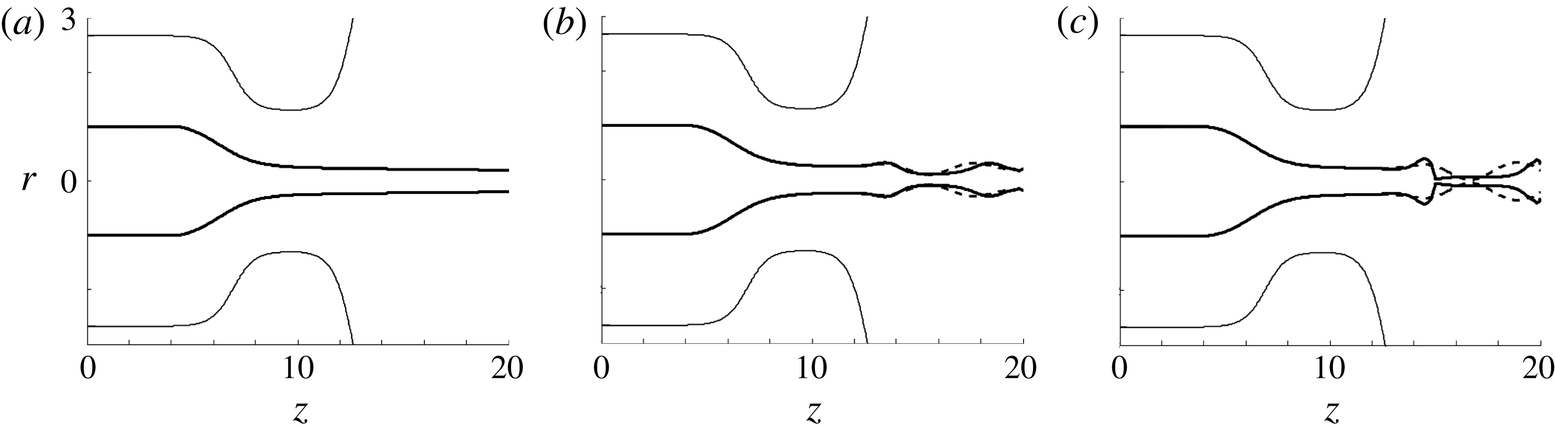
We have integrated the Navier–Stokes equations and boundary conditions linearized around the base flow to examine its short-term response to the impulse with the same governing equations as those of the asymptotic global stability analysis. Figure 10 shows the free surface deformation at three instants for an asymptotically stable base flow. Due to the small magnitude of the perturbation, the free-surface deformation is hardly noticeable at
 $t=0$
. Owing to the non-normal character of the linearized Navier–Stokes operator, the superposition of decaying perturbations triggered by (4.1) gives rise to the free-surface pinch-off within the numerical domain. This kind of short-term convective instability does not cause oscillations of the liquid meniscus, as also shown by both numerical simulations (Herrada et al.
Reference Herrada, Gañán-Calvo, Ojeda-Monge, Bluth and Riesco-Chueca2008) and experiments (Si et al.
Reference Si, Li, Yin and Yin2009; Vega et al.
Reference Vega, Montanero, Herrada and Gañán-Calvo2010) for the plate–orifice flow focusing configuration.
Free-surface deformation calculated with the linearized (dash line) and nonlinear (solid line) hydrodynamic equations at
 $t=0$
(a), 4 (b) and 4.3 (c) for
 $Re_{FF}=40.1$
,
 $We_{FF}=1.21$
and
 $C=0.0136$
.

In the dripping mode of flow focusing, the liquid free surface breaks up at distances from the discharge orifice of the order of its diameter. Therefore, it is reasonable to identify as dripping those simulations where the free surface pinches within our numerical domain, and as jetting otherwise. The solid circles (triangles) in figure 8 correspond to dripping (jetting) flow focusing realizations for water. As can be observed, the short-term convective instability explains the elbow of the stability limit curve for Weber numbers around unity, i.e. why steady jetting becomes unstable and evolves towards dripping for Weber numbers less than unity even if the flow rate is larger than the critical value predicted by the asymptotic stability analysis.
Figure 10 also shows the free-surface deformation when the nonlinear terms of the hydrodynamic equations are taken into account. As can be observed, these terms do not manage to stabilize the perturbation, and the jet’s free surface breaks up next to the liquid source (dripping mode). As expected, only the free-surface pinch-off is affected by nonlinearities, while the latter remain inconsequential in the rest of the numerical domain. Naturally, there is a small jet portion next to the outlet section ‘contaminated’ by the outflow boundary condition (especially in the nonlinear simulation), but this deficiency does not affect the validity of the above conclusions.
5 Conclusions
Modal stability theory lies in the assumption that the linearized Navier–Stokes operator is normal, which guaranties that the energy of small-amplitude perturbations around asymptotically stable base flows decreases monotonously both during the short-term response and the asymptotic regime. However, there can be situations where that condition does not hold (Chomaz Reference Chomaz2005; Schmid Reference Schmid2007). In this case, asymptotic global stability is a necessary but not sufficient condition for stability.
In this work, we have examined numerically the global stability of the steady jetting regime of the axisymmetric gaseous flow focusing. The base flows and the corresponding linear global modes have been calculated from the Navier–Stokes equations to determine the asymptotic stability of those flows. The analysis has been conducted for wide ranges of the liquid viscosity and gas speed (applied pressure drop), and for a geometry similar to that considered in the experiments (Acero et al. Reference Acero, Ferrera, Montanero and Gañán-Calvo2012). The flow rates corresponding to marginal stability agree reasonably well with the experimental values leading to dripping for large enough applied pressure drops. In contrast, these theoretical predictions do not follow the experimental trend for small pressure drops (Weber numbers around and less than unity). To explain this discrepancy, the evolution of small perturbations introduced into the liquid meniscus has been studied by integrating over time the hydrodynamic equations for small gas speeds. We have found that those perturbations can grow while convected by the jet, pinching the free surface next to the discharge orifice. We conclude that the jetting-to-dripping transition is caused by asymptotic global instability for large applied pressure drops, and by the system’s short-term response to perturbations for small values of this parameter.
The present study provides a comprehensive understanding of the flow focusing stability problem, improving previous partial explanations based on local stability analysis (Huerre & Monkewitz Reference Huerre and Monkewitz1990; Eggers & Villermaux Reference Eggers and Villermaux2008; Si et al. Reference Si, Li, Yin and Yin2009; Montanero et al. Reference Montanero, Rebollo-Muñoz, Herrada and Gañán-Calvo2011) and scaling laws (Vega et al. Reference Vega, Montanero, Herrada and Gañán-Calvo2010; Montanero et al. Reference Montanero, Rebollo-Muñoz, Herrada and Gañán-Calvo2011; Acero et al. Reference Acero, Ferrera, Montanero and Gañán-Calvo2012). The analysis can extended to a number of similar microfluidic configurations, including coflow systems, electrospray, liquid–liquid flow focusing, ….
Acknowledgement
This research has been supported by the Spanish Ministry of Economy, Industry and Competitiveness under grant DPI2016-78887.