1 Introduction
Wakes in the natural environment are associated with engineered devices, e.g. ships, underwater submersibles, aircraft, unmanned aerial vehicles and wind turbines, with marine swimmers and aerial flyers and with topographic features such as islands and mountains. Stratification of the environment affects these wakes leading to distinctive features. A comprehensive review of experimental studies prior to 1979 is given by Lin & Pao (Reference Lin and Pao1979) while the recent review by Spedding (Reference Spedding2014) includes later work with an emphasis on laboratory experiments while also considering wakes of marine animals as well as geophysical examples.
Lin & Pao (Reference Lin and Pao1979) reviewed high-
 $Fr$
wakes with
 $Fr=O$
(10–1000) and concluded that, after
 $Nt=O(1)$
, buoyancy qualitatively changes the structure of the wake through the inhibition of vertical motion. Here,
 $Fr=U_{\infty }/ND$
where
 $U_{\infty }$
is the speed of the free-stream fluid relative to the body,
 $D$
is the body diameter,
 $N$
is the background value of the buoyancy frequency and
 $t=x/U_{\infty }$
is the time that corresponds to streamwise distance
 $x$
from the body. Their visualizations for slender-body, high-
 $Fr$
flows show wake contraction and the formation of large-scale vortices in the horizontal flow. Lin, Boyer & Fernando (Reference Lin, Boyer and Fernando1992a
) studied the behaviour of flow past a sphere for
 $Re=[5,10\,000]$
and
 $Fr=[0.005,15]$
, finding a turbulent wake for
 $Re>2000$
and sufficiently high
 $Fr$
. They report that the vertical and the horizontal thickness of wakes with
 $Fr\gtrsim 2$
grow similarly following a
 $t^{1/3}$
law (the classical self-similar behaviour of an unstratified round wake) until
 $Nt\approx 2$
, where the vertical thickness reaches its maximum. After
 $Nt\approx 2$
, the vertical wake thickness normalized by
 $D$
becomes
 $O(1)$
, whereas in the horizontal direction it increases as
 $t^{1/2}$
. It is worth noting that the scalings proposed by Lin & Pao (Reference Lin and Pao1979) were based on shadowgraph visualizations and not quantitative velocity measurements.
Hanazaki (Reference Hanazaki1988) used direct numerical simulation (DNS) to study flow past a sphere at a relatively low
 $Re=200$
and
 $Fr_{R}=[0.25,200]$
(
 $Fr_{R}=U_{\infty }/NR$
, where
 $R$
is the sphere radius). They found steady flow with an attached separation bubble and discussed the effect of the steady lee wave pattern on flow separation and drag coefficient. Flow past a sphere at higher
 $Re$
that allows unsteadiness was investigated experimentally by Chomaz et al. (Reference Chomaz, Bonneton, Butet, Perrier and Hopfinger1992), Lin et al. (Reference Lin, Lindberg, Boyer and Fernando1992b
) and Chomaz, Bonneton & Hopfinger (Reference Chomaz, Bonneton and Hopfinger1993a
). These authors describe how flow separation, vortex shedding and the lee wave pattern change significantly as the flow conditions change among the regimes of low
 $Fr$
,
 $Fr=O(1)$
and high
 $Fr$
. Depending on the strength of the stratification, the internal wave field consists of lee waves generated by the body and random internal waves generated by the turbulent wake. Investigations of these lee and random waves have been performed using experimental (Gilreath & Brandt Reference Gilreath and Brandt1985; Hopfinger et al.
Reference Hopfinger, Flor, Chomaz and Bonneton1991; Bonneton, Chomaz & Hopfinger Reference Bonneton, Chomaz and Hopfinger1993; Chomaz et al.
Reference Chomaz, Bonneton and Hopfinger1993a
; Bonneton et al.
Reference Bonneton, Chomaz, Hopfinger and Perrier1996; Brandt & Rottier Reference Brandt and Rottier2015), numerical (Abdilghanie & Diamessis Reference Abdilghanie and Diamessis2013; Zhou & Diamessis Reference Zhou and Diamessis2016) and theoretical techniques (Voisin Reference Voisin1991, Reference Voisin1994, Reference Voisin2007).
The late-wake evolution in the horizontal centre plane of the wake of a sphere towed in a stratified fluid was investigated by Spedding, Browand & Fincham (Reference Spedding, Browand and Fincham1996) at
 $Re=[10^{3},10^{4}]$
and
 $Fr_{R}=[1,10]$
using digital particle image velocimetry (DPIV). For
 $Re>5000$
, the streamwise average of quantities such as normalized fluctuation velocity, vorticity magnitude and energy dissipation rate exhibited power-law scalings similar to that of axisymmetric turbulent wakes. The stratified wakes spread horizontally with a growth rate of
 $t^{1/3}$
similar to the self-similar, unstratified wake while the defect velocity was an order of magnitude larger than the unstratified case. As in previous experiments, the late wake was dominated by coherent vortices. Spedding (Reference Spedding1997) expanded the study to the high-
 $Fr$
regime,
 $Fr_{R}=[10,240]$
, and identified a non-equilibrium (NEQ) phase that commences at
 $Nt\simeq 2$
, during which the initial near-wake (NW) turbulence feels the influence of the background density gradient and the mean velocity decay of the wake is substantially reduced by buoyancy to approximately
 $(Nt)^{-0.25}$
. There is an eventual transition to a quasi-two-dimensional (Q2-D) phase where the flow is constrained in the vertical direction owing to the effect of buoyancy, pancake vortices emerge and the mean velocity decays as approximately
 $(Nt)^{-0.76}$
, faster than in the NEQ regime. Bonnier & Eiff (Reference Bonnier and Eiff2002) experimentally studied sphere wakes at
 $(Fr_{R},Re)=(3,3400),(6,6900),(10,11\,500)$
and found an ‘accelerated collapse’ phase with an abrupt increase in the centreline defect velocity at
 $Nt\approx 3$
that lasted for
 $\unicode[STIX]{x0394}Nt\approx 5$
.
Numerical simulations that have been performed in the past two decades to study stratified sphere wakes have primarily used the temporally evolving model, wherein periodic boundary conditions are used in the streamwise direction and the wake statistics are a function of time. The simulation is initialized with a synthetic velocity field that satisfies assumed profiles for the mean and variance. These profiles are typically taken to approximate unstratified wake measurements a few body diameters downstream of the sphere. In contrast, the spatially evolving model allows streamwise evolution of the flow statistics and thus has the ability to include the body and near-wake dynamics. Temporal wake simulations commenced with the DNS of Gourlay et al. (Reference Gourlay, Arendth, Fritts and Werne2001) who simulated a wake at nominal
 $Re=10^{4}$
and
 $Fr=10$
on a grid with 162 million grid points. A conclusion was that pancake eddies form in the late wake, independent of the absence in the initial conditions of coherent fluctuations associated with vortex shedding off the body. Later numerical studies of wake statistics, turbulence budgets and vortex dynamics include the large eddy simulations (LES) by Dommermuth et al. (Reference Dommermuth, Rottman, Innis and Novikov2002) at
 $Re=10^{4},10^{5}$
and
 $Fr=2$
with improved initial conditions, the DNS by Brucker & Sarkar (Reference Brucker and Sarkar2010) of towed and self-propelled wakes at
 $Re=10^{4}$
and
 $Re=5\times 10^{4}$
, using a grid with up to 2 billion grid points, the implicit LES of Diamessis, Spedding & Domaradzki (Reference Diamessis, Spedding and Domaradzki2011) conducted over a wide range of
 $Fr$
and
 $Re$
and DNS of a weakly stratified wake with
 $Fr=65$
by Redford, Lund & Coleman (Reference Redford, Lund and Coleman2015). At high
 $Re$
, the NEQ regime has enhanced turbulence owing to secondary Kelvin–Helmholtz (KH) instabilities (Diamessis et al.
Reference Diamessis, Spedding and Domaradzki2011) and the duration of the NEQ regime is extended (Brucker & Sarkar Reference Brucker and Sarkar2010). By quantification of the mean wake energetics, Brucker & Sarkar (Reference Brucker and Sarkar2010) found that, owing to the buoyancy-induced reduction of Reynolds shear stress of the vertical velocity, the turbulent production responsible for the transfer of energy from mean to fluctuations is reduced, thus leading to defect velocity in the NEQ regime that is substantially higher than in the unstratified wake. This explanation for the longer lifetime of stratified wakes was confirmed by Redford et al. (Reference Redford, Lund and Coleman2015) who also found that the robust Reynolds shear stress associated with quasi-two-dimensional motions leads to a faster (relative to the NEQ regime) decay of the mean wake velocity in the Q2-D regime. Meunier, Diamessis & Spedding (Reference Meunier, Diamessis and Spedding2006) developed a scaling model based on the self-similarity of the near wake. However, in the present simulations it is found that the dynamics of the near wake is significantly altered by the presence of the body. Pal & Sarkar (Reference Pal and Sarkar2015) examined the effect of external fluctuations finding that, although the wake turbulence was enhanced and the decay of the wake defect velocity was somewhat increased, the stratified wake was still long lived relative to its unstratified counterpart. Watanabe et al. (Reference Watanabe, Riley, de Bruyn Kops, Diamessis and Zhou2016) found the turbulent/non-turbulent interface to have a thickness characterized by the Kolmogorov scale and to have a
 $O(1)$
buoyancy Reynolds number in their DNS study.
Abdilghanie & Diamessis (Reference Abdilghanie and Diamessis2013) characterized the near-field properties of the wake-radiated internal waves and found that the internal wave emission is prolonged over a longer time interval at high
 $Re$
. Zhou & Diamessis (Reference Zhou and Diamessis2016), in contrast to Abdilghanie & Diamessis (Reference Abdilghanie and Diamessis2013), focused on the far-field (surface/near-surface) properties of the wake-radiated internal waves and found that, at higher Reynolds numbers, all of the wave flux originates from the near wake and not the stratified turbulence that follows. Brucker & Sarkar (Reference Brucker and Sarkar2010), in their examination of the turbulent kinetic energy (TKE) budget in a
 $Fr=4$
,
 $Re=50\,000$
wake, found that the internal wave flux exceeded the turbulent dissipation rate during
 $20<Nt<75$
. Watanabe et al. (Reference Watanabe, Riley, de Bruyn Kops, Diamessis and Zhou2016) also find that the internal wave flux is larger than the turbulent dissipation at
 $Nt=21$
in their high-
 $Re$
case, but it is smaller in their low-
 $Re$
case.
DNS of the turbulent wake in a computational model which includes the body is relatively recent. The unstratified case was studied using DNS by Rodriguez et al. (Reference Rodriguez, Borelli, Lehmkuhl, Perez Segarra and Oliva2011) at
 $Re=3700$
who used an unstructured grid. Vortex shedding at a Strouhal number of
 $St=0.215$
(
 $St=U_{\infty }\,f/D$
, where
 $f$
is the frequency) occurred at random azimuthal positions leading to a helical-like configuration of the downstream wake. Passive scalar mixing was studied by de Stadler, Rapaka & Sarkar (Reference de Stadler, Rapaka and Sarkar2014) who performed LES of a heated sphere at
 $Re=10\,000$
. Bazilevs et al. (Reference Bazilevs, Yan, de Stadler and Sarkar2014) in their simulation of flow past a sphere at
 $Re=3700$
found that, due to the free-stream turbulence in the inlet conditions, the near-wake turbulence is substantially increased, the recirculation bubble decreases significantly and the drag force on the sphere is increased. Temporal evolution of the far wake of a sphere in a stratified fluid, using the initial condition from a spatially evolving simulation, was carried out by Pasquetti (Reference Pasquetti2011) at
 $Re=10^{4}$
and
 $Fr=25$
. Orr et al. (Reference Orr, Domaradzki, Spedding and Constantinescu2015) numerically investigated flow over a sphere at
 $Re=200,1000$
and
 $1\leqslant Fr\leqslant \infty$
using body-fitted grids. They provided parametrization of the near wake based on the wake height, the downstream distance and
 $Fr$
. Simulations of flow past a sphere at
 $Re=3700$
in the high-stratification regime of
 $Fr<O(1)$
have been reported by Pal et al. (Reference Pal, Sarkar, Posa and Balaras2016). Buoyancy suppressed turbulence so that by
 $Fr=0.5$
, there is negligible unsteadiness in the wake. However, further decrease of
 $Fr$
below approximately 0.25 results in regeneration of turbulence owing to a new regime of vortex shedding. A discussion of the coherent structures and the enstrophy dynamics in these low-
 $Fr$
sphere wakes is provided by Chongsiripinyo, Pal & Sarkar (Reference Chongsiripinyo, Pal and Sarkar2016).
A temporal approximation requires an approximation of the initial fluctuations some distance from the body where the free-stream velocity is much higher than the wake defect velocity. For moderately stratified wakes with
 $Fr=O(1)$
, the transition to the NEQ regimes occurs with a few body lengths and the temporal approximation would require initial conditions very different from the customary choice that is based on unstratified flow. More generally, the somewhat ad hoc initial conditions used in the temporal simulations cannot be expected to capture the near-wake characteristics and the early NEQ regime since the details of the near-body flow could affect the vortex dynamics, turbulence and wave emission in that region. Spatial simulations with proper resolution near the body can also capture the boundary layer dynamics, the effect of vortex shedding on stratified wakes and help understand the evolution of the near wake into the NEQ regime, including the possible presence of the acceleration of the wake defect velocity that was reported by Bonnier & Eiff (Reference Bonnier and Eiff2002).
The present study is a numerical investigation of flow over a sphere at moderate Reynolds number,
 $Re=3700$
, for which both DNS and experimental data are available for validation in the unstratified case. We focus on moderate stratification of
 $Fr=O(1)$
and simulate flows with
 $Fr=1,2,3$
and
 $\infty$
. To the authors best knowledge, this is the first numerical study of turbulent flow past a sphere in a stably stratified environment which resolves small scales near the body and systematically investigates buoyancy effects in the
 $Fr=O(1)$
regime on near-, intermediate- and far-wake behaviour. We simulate the flow up to a downstream length of
 $x_{1}/D\approx 80$
, and quantify wake characteristics in the near and NEQ regime such as defect velocity and its scaling, turbulence levels and spectra and compare the time-averaged turbulent kinetic energy TKE budget terms with the benchmark unstratified case. We defer a detailed discussion of internal wave properties to follow-up work.
2 Problem formulation
Turbulent wakes can be simulated either in a temporally evolving or in a spatially evolving model. In a temporal model, the wake is initialized by an assumed mean velocity profile with superposed turbulent fluctuations that satisfy a given spectrum, and the subsequent time evolution of the flow is captured in a domain with periodic boundary conditions in the streamwise direction. This method of simulating wakes is relatively inexpensive since the boundary layer and its separation are not resolved and, therefore, higher Reynolds number and Froude numbers can be achieved (Brucker & Sarkar Reference Brucker and Sarkar2010; Diamessis et al.
Reference Diamessis, Spedding and Domaradzki2011). Nevertheless, the flow is dependent on the type of initial conditions (the initial mean wake velocity profiles and the fluctuations), a limitation that can be overcome through spatially evolving simulations that include the body. The downstream distance
 $x_{1}$
in spatially evolving simulations is related to the time
 $t$
of evolution in the temporal simulations via the relation
 $x_{1}=U_{\infty }t$
(Gourlay et al.
Reference Gourlay, Arendth, Fritts and Werne2001; Brucker & Sarkar Reference Brucker and Sarkar2010; Pal, de Stadler & Sarkar Reference Pal, de Stadler and Sarkar2013; Pal Reference Pal2016). The buoyancy time period
 $Nt$
and the non-dimensional downstream length
 $x_{1}/D$
can be related using
 $Nt=x_{1}/FrD$
. Body-inclusive spatial DNS is expensive owing to the fine grid required to resolve the boundary layer near the body and is limited in practice to moderate Reynolds numbers and moderate domain size in the streamwise direction.
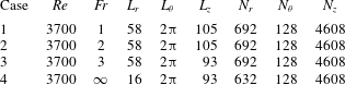
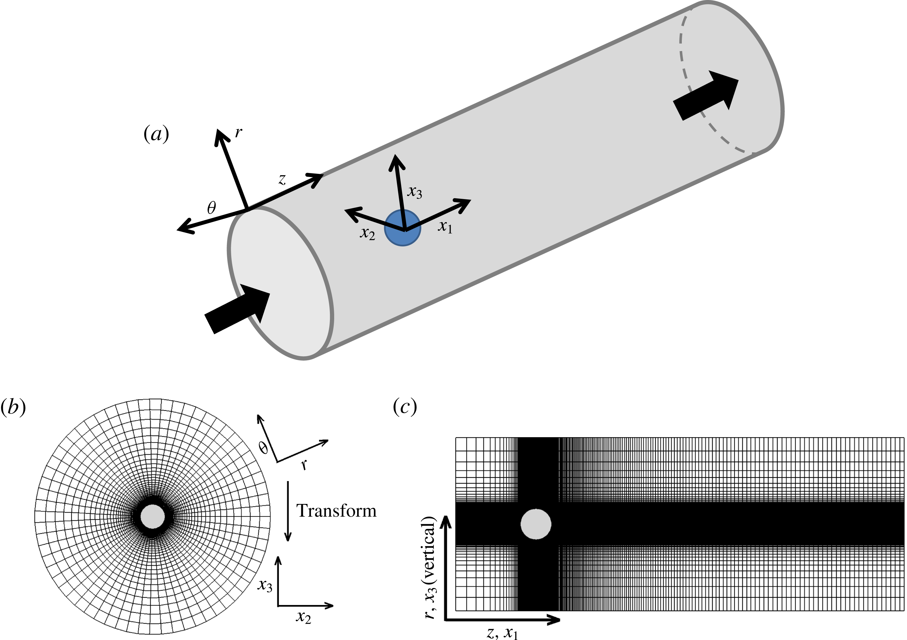
Table 1 shows the various simulation parameters including domain dimensions and grid dimensions. The sphere is embedded at the origin of a cylindrical computational domain, as shown by figure 1. High resolution is used at the sphere surface (20 points across the boundary layer thickness at the point of maximum wall shear stress) and in the wake. The radial grid spacing is
 $\unicode[STIX]{x0394}r/D\simeq 0.0016$
in the cylindrical region (
 $r/D<0.65$
) that encloses the sphere, the azimuthal direction has 128 points and
 $\unicode[STIX]{x0394}z/D\simeq 0.0016$
near the surface. The grid has mild stretching, radially and streamwise, away from the body. The radial spacing is less than the Kolmogorov scale,
 $\unicode[STIX]{x1D702}$
, over the entire wake. The streamwise grid spacing, after reaching approximately
 $1.5\unicode[STIX]{x1D702}$
near the body decreases to below
 $\unicode[STIX]{x1D702}$
after
 $x_{1}/D\approx 60$
. The azimuthal grid spacing,
 $r\unicode[STIX]{x0394}\unicode[STIX]{x1D703}$
, at
 $r=0.5$
has a maximum of approximately
 $4\unicode[STIX]{x1D702}$
in the separated shear layer at
 $x_{1}/D=2$
; the resolution then improves to
 $2.7\unicode[STIX]{x1D702}$
at
 $x_{1}/D=5$
and to less than
 $2\unicode[STIX]{x1D702}$
by
 $x_{1}/D=10$
. Radially outward at
 $r/D=2$
, the resolution improves to
 $r/D\unicode[STIX]{x0394}\unicode[STIX]{x1D703}<\unicode[STIX]{x1D702}$
for all streamwise locations.
Simulation parameters.

Schematic of the simulation set-up: (a) three-dimensional cylindrical domain with the sphere at
 $(0,0,0)$
and uniform inflow in the
 $x_{1}$
direction, (b)
 $r{-}\unicode[STIX]{x1D703}$
cross-section, skipping 5 points in
 $r/D$
and 1 point in
 $\unicode[STIX]{x1D703}$
; and (c)
 $r{-}z$
cross-section, skipping 10 points in both
 $r/D$
and
 $z/D$
directions. Portions of the computational domain, rather than the entirety, are shown for clarity.

The temporal simulations of Gourlay et al. (Reference Gourlay, Arendth, Fritts and Werne2001) and Brucker & Sarkar (Reference Brucker and Sarkar2010) have shown evolution of a towed wake for
 $t\in [10^{2}{-}10^{5}]$
whereas Pal et al. (Reference Pal, de Stadler and Sarkar2013) has presented spatial simulations (without including the body) of a self-propelled wake for a downstream distance of
 $x_{1}/D\sim 240$
. Note that although very long time evolution and moderate downstream distances are achieved in these previous simulations, the effect of a body on the evolution of a stratified wake is still unexplored. The present simulations not only include a sphere, but show the wake evolution up to a downstream domain length of
 $x_{1}/D\approx 80$
. The domain is extended in the upstream direction to accommodate upstream wave propagation. For
 $Fr=1$
and 2, an upstream distance of 25 is used relative to a shorter upstream length of 13 for
 $Fr=3$
which has weaker body-generated waves. To prevent spurious reflection back into the domain from these upstream propagating body-generated waves and from the turbulence-generated internal gravity waves, we use an inlet sponge and a cylindrical sponge at the domain boundary.
2.1 Governing equations and numerical method
The governing equations are the three-dimensional incompressible, unsteady form of the conservation equations for mass, momentum and density, respectively, subject to the Boussinesq approximation for buoyancy. They take the following form in a cylindrical coordinate system:
 $$\begin{eqnarray}\displaystyle & \displaystyle \frac{1}{r}\frac{\unicode[STIX]{x2202}(ru_{r})}{\unicode[STIX]{x2202}r}+\frac{1}{r}\frac{\unicode[STIX]{x2202}u_{\unicode[STIX]{x1D703}}}{\unicode[STIX]{x2202}\unicode[STIX]{x1D703}}+\frac{\unicode[STIX]{x2202}u_{z}}{\unicode[STIX]{x2202}z}=0, & \displaystyle\end{eqnarray}$$
 $$\begin{eqnarray}\displaystyle & \displaystyle \frac{\unicode[STIX]{x2202}u_{r}}{\unicode[STIX]{x2202}t}+(\boldsymbol{u}\boldsymbol{\cdot }\unicode[STIX]{x1D735})u_{r}-\frac{u_{\unicode[STIX]{x1D703}}^{2}}{r}=-\frac{1}{\unicode[STIX]{x1D70C}_{0}}\frac{\unicode[STIX]{x2202}p}{\unicode[STIX]{x2202}r}+\unicode[STIX]{x1D708}\left(\unicode[STIX]{x1D6FB}^{2}u_{r}-\frac{u_{r}}{r^{2}}-\frac{2}{r^{2}}\frac{\unicode[STIX]{x2202}u_{\unicode[STIX]{x1D703}}}{\unicode[STIX]{x2202}\unicode[STIX]{x1D703}}\right)+\frac{\widetilde{\unicode[STIX]{x1D70C}}}{\unicode[STIX]{x1D70C}_{0}}g_{r}, & \displaystyle\end{eqnarray}$$
 $$\begin{eqnarray}\displaystyle & \displaystyle \frac{\unicode[STIX]{x2202}u_{\unicode[STIX]{x1D703}}}{\unicode[STIX]{x2202}t}+(\boldsymbol{u}\boldsymbol{\cdot }\unicode[STIX]{x1D735})u_{\unicode[STIX]{x1D703}}+\frac{u_{r}u_{\unicode[STIX]{x1D703}}^{2}}{r}=-\frac{1}{\unicode[STIX]{x1D70C}_{0}r}\frac{\unicode[STIX]{x2202}p}{\unicode[STIX]{x2202}\unicode[STIX]{x1D703}}+\unicode[STIX]{x1D708}\left(\unicode[STIX]{x1D6FB}^{2}u_{\unicode[STIX]{x1D703}}-\frac{u_{\unicode[STIX]{x1D703}}}{r^{2}}+\frac{2}{r^{2}}\frac{\unicode[STIX]{x2202}u_{r}}{\unicode[STIX]{x2202}\unicode[STIX]{x1D703}}\right)+\frac{\widetilde{\unicode[STIX]{x1D70C}}}{\unicode[STIX]{x1D70C}_{0}}g_{\unicode[STIX]{x1D703}}, & \displaystyle\end{eqnarray}$$
 $$\begin{eqnarray}\displaystyle & \displaystyle \frac{\unicode[STIX]{x2202}u_{z}}{\unicode[STIX]{x2202}t}+(\boldsymbol{u}\boldsymbol{\cdot }\unicode[STIX]{x1D735})u_{z}=-\frac{1}{\unicode[STIX]{x1D70C}_{0}}\frac{\unicode[STIX]{x2202}p}{\unicode[STIX]{x2202}z}+\unicode[STIX]{x1D708}\unicode[STIX]{x1D6FB}^{2}u_{z}, & \displaystyle\end{eqnarray}$$
 $$\begin{eqnarray}\displaystyle & \displaystyle \frac{\unicode[STIX]{x2202}\unicode[STIX]{x1D70C}}{\unicode[STIX]{x2202}t}+(\boldsymbol{u}\boldsymbol{\cdot }\unicode[STIX]{x1D735})\unicode[STIX]{x1D70C}=\unicode[STIX]{x1D705}\unicode[STIX]{x1D6FB}^{2}\unicode[STIX]{x1D70C}, & \displaystyle\end{eqnarray}$$
where
 $u_{r}$
,
 $u_{\unicode[STIX]{x1D703}}$
and
 $u_{z}$
are the velocities in the radial, azimuthal and the streamwise directions, respectively,
 $p$
is the pressure,
 $\unicode[STIX]{x1D708}$
is the kinematic viscosity,
 $g_{r}=g\sin \unicode[STIX]{x1D703}$
and
 $g_{\unicode[STIX]{x1D703}}=g\cos \unicode[STIX]{x1D703}$
are the components of gravity (
 $g$
) in the radial and azimuthal direction respectively and
 $\unicode[STIX]{x1D705}$
is the molecular diffusivity. The density is given by
 $$\begin{eqnarray}\unicode[STIX]{x1D70C}=\unicode[STIX]{x1D70C}_{bg}(x_{3})+\widetilde{\unicode[STIX]{x1D70C}}(r,\unicode[STIX]{x1D703},z,t),\end{eqnarray}$$
where
 $\unicode[STIX]{x1D70C}_{bg}(x_{3})$
is the fixed background density that varies linearly in the vertical direction
 $x_{3}$
and the density deviation,
 $\widetilde{\unicode[STIX]{x1D70C}}(r,\unicode[STIX]{x1D703},z,t)$
, appears in the momentum equation. In the cylindrical coordinate system,
 $\unicode[STIX]{x1D70C}_{bg}(x_{3})=\unicode[STIX]{x1D70C}_{0}+\unicode[STIX]{x1D70C}^{\ast }(r,\unicode[STIX]{x1D703})$
.
The governing equations are solved numerically in a cylindrical coordinate system on staggered grids. The sphere inside the domain is represented by an immersed boundary method following Balaras (Reference Balaras2004), Yang & Balaras (Reference Yang and Balaras2006). Use of a cylindrical coordinate system rather than a planar coordinate system improves approximation of the sphere surface and the gradients in the boundary layer. For the time advancement a semi-implicit, Runge–Kutta/Crank–Nicolson formulation is used, where all the terms in the azimuthal direction are treated implicitly to eliminate restrictions to the time step due to small values of
 $r\unicode[STIX]{x0394}\unicode[STIX]{x1D703}$
near the axis. All remaining terms are advanced explicitly. All spatial derivatives are discretized using a central, second-order, finite difference scheme on a staggered grid. The pressure Poisson equation, which is utilized to project the velocity field into a divergence-free space, is solved using direct methods. In particular, trigonometric transforms in the azimuthal direction are used to reduce the problem into a set of penta-diagonal matrices, which are then solved directly with a divide and conquer strategy (Rossi & Toivanen Reference Rossi and Toivanen1999). The velocities obtained by solving the governing equations are converted to Cartesian coordinates by using the following transformation:
 $$\begin{eqnarray}\left[\begin{array}{@{}c@{}}u_{1}\\ u_{2}\\ u_{3}\end{array}\right]=\left[\begin{array}{@{}ccc@{}}0 & 0 & 1\\ \cos \unicode[STIX]{x1D703} & -\sin \unicode[STIX]{x1D703} & 0\\ \sin \unicode[STIX]{x1D703} & \cos \unicode[STIX]{x1D703} & 0\end{array}\right]\times \left[\begin{array}{@{}c@{}}u_{r}\\ u_{\unicode[STIX]{x1D703}}\\ u_{z}\end{array}\right],\end{eqnarray}$$
where
 $u_{1}$
,
 $u_{2}$
and
 $u_{3}$
are the velocities in the streamwise, horizontal and vertical directions respectively. The derivatives of a variable
 $\unicode[STIX]{x1D719}$
in the Cartesian coordinate system can be calculated from the corresponding derivatives in the cylindrical coordinate system as follows
 $$\begin{eqnarray}\left[\begin{array}{@{}c@{}}{\displaystyle \frac{\unicode[STIX]{x2202}\unicode[STIX]{x1D719}}{\unicode[STIX]{x2202}x_{1}}}\\ {\displaystyle \frac{\unicode[STIX]{x2202}\unicode[STIX]{x1D719}}{\unicode[STIX]{x2202}x_{2}}}\\ {\displaystyle \frac{\unicode[STIX]{x2202}\unicode[STIX]{x1D719}}{\unicode[STIX]{x2202}x_{3}}}\end{array}\right]=\left[\begin{array}{@{}ccc@{}}0 & 0 & 1\\ \cos \unicode[STIX]{x1D703} & {\displaystyle \frac{-\sin \unicode[STIX]{x1D703}}{r}} & 0\\ \sin \unicode[STIX]{x1D703} & {\displaystyle \frac{\cos \unicode[STIX]{x1D703}}{r}} & 0\end{array}\right]\times \left[\begin{array}{@{}c@{}}{\displaystyle \frac{\unicode[STIX]{x2202}\unicode[STIX]{x1D719}}{\unicode[STIX]{x2202}r}}\\ {\displaystyle \frac{\unicode[STIX]{x2202}\unicode[STIX]{x1D719}}{\unicode[STIX]{x2202}\unicode[STIX]{x1D703}}}\\ {\displaystyle \frac{\unicode[STIX]{x2202}\unicode[STIX]{x1D719}}{\unicode[STIX]{x2202}z}}\end{array}\right].\end{eqnarray}$$
2.2 Calculation of statistics
Statistics are computed using time averaging of the data over an interval that spans approximately 80 non-dimensional time units (
 $tU_{\infty }/D$
) after the flow has reached statistical steady state at approximately 120 time units. The Reynolds decomposition into mean and fluctuations is
 $$\begin{eqnarray}u_{i}=\langle u_{i}\rangle +u_{i}^{\prime },\quad \unicode[STIX]{x1D70C}=\langle \unicode[STIX]{x1D70C}\rangle +\unicode[STIX]{x1D70C}^{\prime },\quad p=\langle p\rangle +p^{\prime }.\end{eqnarray}$$
Statistics in the stratified wake are a function of streamwise (
 $x_{1}$
), horizontal (
 $x_{2}$
) and vertical (
 $x_{3}$
) directions.
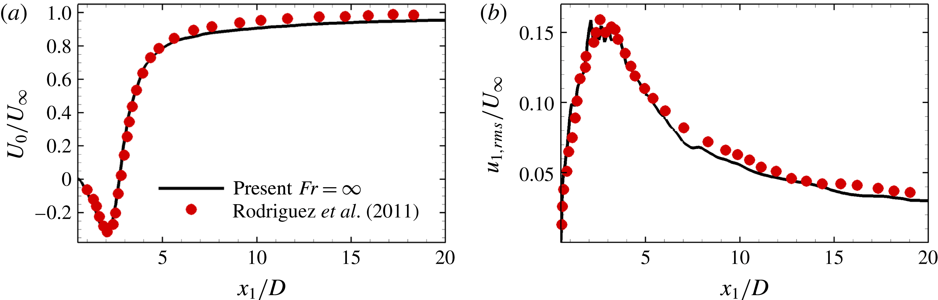
Comparison of the unstratified wake. Streamwise evolution at the centreline (
 $x_{2}=0$
and
 $x_{3}=0$
) of: (a) mean defect velocity and (b) root mean square (r.m.s.) streamwise velocity.

Validation of the numerical method and grid resolution of the present DNS against previous experimental and numerical results are presented in Pal et al. (Reference Pal, Sarkar, Posa and Balaras2016). A match is found for the vortex shedding frequency,
 $St=fD/U_{\infty }$
, separation angle,
 $\unicode[STIX]{x1D711}_{s}$
, drag coefficient,
 $C_{d}$
, rearward stagnation pressure coefficient,
 $C_{pb}$
with the previous investigations (Schlichting Reference Schlichting1968; Kim & Durbin Reference Kim and Durbin1988; Sakamoto & Haniu Reference Sakamoto and Haniu1990; Seidl, Muzaferija & Perić Reference Seidl, Muzaferija and Perić1997; Tomboulides & Orszag Reference Tomboulides and Orszag2000; Constantinescu & Squires Reference Constantinescu and Squires2003; Yun, Kim & Choi Reference Yun, Kim and Choi2006; Rodriguez et al.
Reference Rodriguez, Borelli, Lehmkuhl, Perez Segarra and Oliva2011) as discussed in Pal et al. (Reference Pal, Sarkar, Posa and Balaras2016). It was shown previously by us that the pressure coefficient,
 $C_{p}(\unicode[STIX]{x1D703})$
plotted in figure 1(a) of Pal et al. (Reference Pal, Sarkar, Posa and Balaras2016), agreed well with the DNS of Rodriguez et al. (Reference Rodriguez, Borelli, Lehmkuhl, Perez Segarra and Oliva2011) and the experiment of Kim & Durbin (Reference Kim and Durbin1988). The friction coefficient,
 $C_{f}(\unicode[STIX]{x1D703})$
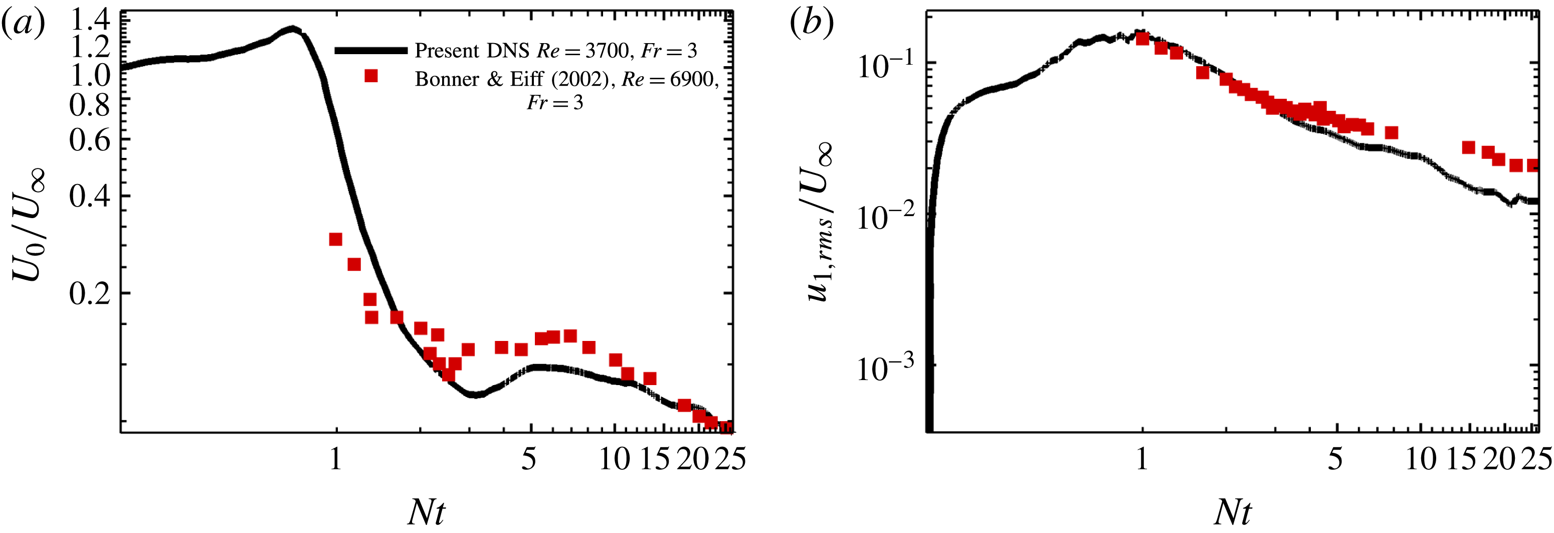
plotted in figure 1(b) of Pal et al. (Reference Pal, Sarkar, Posa and Balaras2016), agreed well with the simulations of Seidl et al. (Reference Seidl, Muzaferija and Perić1997) and Rodriguez et al. (Reference Rodriguez, Borelli, Lehmkuhl, Perez Segarra and Oliva2011). Comparison of the streamwise mean defect and r.m.s. velocity at the centreline with Rodriguez et al. (Reference Rodriguez, Borelli, Lehmkuhl, Perez Segarra and Oliva2011) is good as demonstrated by figure 2. We have also compared the evolution of the streamwise mean defect velocity and r.m.s. velocity at the centreline with the experimental results of Bonnier & Eiff (Reference Bonnier and Eiff2002) that were obtained with a hot-film probe. The value of
 $Fr=U/ND=3$
is the same between the simulation and the experiment although the
 $Re=6900$
of the experiment is higher. As shown in figure 3 the essential features of the wake evolution in the DNS are quantitatively similar to the experiments of Bonnier & Eiff (Reference Bonnier and Eiff2002).
Validation of the stratified wake. Streamwise evolution at the centreline (
 $x_{2}=0$
and
 $x_{3}=0$
) of: (a) mean defect velocity and (b) r.m.s. streamwise velocity.

3 Visualization of the flow past a sphere
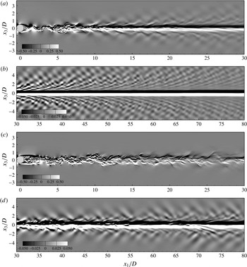
Figure 4(a,b) shows contour plots of the azimuthal vorticity in the vertical
 $x_{1}{-}x_{3}$
centre plane for the
 $Fr=1$
case at
 $0.5<x_{1}/D<30$
and
 $30<x_{1}/D<80$
, respectively. The analogous plots for
 $Fr=3$
are shown in 4(c) and 4(d), respectively. The separating shear layer at
 $Fr=1$
(figure 4
a) remains laminar and plunges towards the centreline at
 $x_{1}/D\approx 1.5$
owing to the strong restoring effect of buoyancy resulting in a significantly shorter recirculation region in comparison to the
 $Fr=3$
(figure 4
c) case. Downstream of
 $x_{1}/D\approx 10$
, the azimuthal vorticity takes a smooth two-layered form suggesting the decay of broadband fluctuations (confirmed by spectra). The evolution of azimuthal vorticity at
 $Fr=3$
is qualitatively different. The shear layer is able to roll up before buoyancy forces a less abrupt but still noticeable plunge of the shear layer towards the centreline which, as shown by figure 4(c), occurs at
 $x_{1}/D\approx 4.5$
. Interestingly, for both
 $Fr=1$
and 3, the curving of the shear layer towards the centreline occurs at the same value of buoyancy time,
 $Nt\approx 1.5$
. Unlike the
 $Fr=1$
case, the vorticity in figure 4(c) has small-scale content throughout
 $0<x_{1}/D<30$
. Phase lines indicative of internal wave emission from the wake into the background are seen for both cases. Closer inspection shows that the signature of the internal waves start at
 $x_{1}/D\approx 7$
for
 $Fr=1$
and
 $x_{1}/D\approx 21$
for
 $Fr=3$
as shown in figures 4(a) and 4(c), respectively. In terms of the buoyancy period, this location corresponds to
 $Nt=7$
for both
 $Fr=1$
and 3. The properties of these wake-generated waves will be described in a follow-up to the present work.
Instantaneous azimuthal vorticity on the vertical centre plane: (a)
 $Fr=1$
,
 $-0.5<x_{1}/D<30$
, (b)
 $Fr=1$
,
 $30<x_{1}/D<80$
, (c)
 $Fr=3$
,
 $-0.5<x_{1}/D<30$
and (d)
 $Fr=3$
,
 $30<x_{1}/D<80$
.

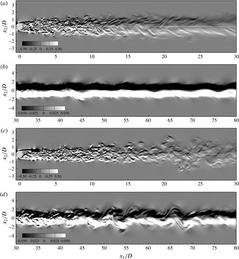
The azimuthal vorticity contour plots in the horizontal
 $x_{1}-x_{2}$
centre plane for
 $Fr=1$
at
 $0.5<x_{1}/D<30$
and
 $30<x_{1}/D<80$
are shown in figures 5(a) and 5(b), respectively, and the corresponding plots for
 $Fr=3$
are shown in 5(c) and 5(d), respectively. The anisotropy of the wake, i.e. larger horizontal spread relative to the vertical spread, is evident in both cases and more so in the
 $Fr=1$
case. Figure 5(a) shows that the shear layer rolls up in the horizontal plane and becomes turbulent in contrast to the quasi-laminar behaviour in the vertical plane. In general, there is stronger variability in the horizontal motion relative to motion in the vertical plane. The vertical vorticity is organized into coherent vortical structures further downstream,
 $30<x_{1}/D<80$
, in the
 $Fr=3$
case. In contrast, the corresponding plot for
 $Fr=1$
exhibits a quasi-steady double-layered distribution.
Instantaneous azimuthal vorticity on the horizontal centerplane: (a)
 $Fr=1$
,
 $-0.5<x_{1}/D<30$
, (b)
 $Fr=1$
,
 $30<x_{1}/D<80$
, (c)
 $Fr=3$
,
 $-0.5<x_{1}/D<30$
and (d)
 $Fr=3$
,
 $30<x_{1}/D<80$
.

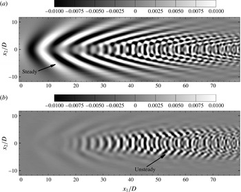
Figure 6(a) shows the total internal wave field for
 $Fr=1$
visualized through the contour plots of vertical strain (
 $\unicode[STIX]{x2202}u_{3}/\unicode[STIX]{x2202}x_{3}$
) on a horizontal plane at a vertical height of
 $x_{3}/D=5$
and at time
 $t=138$
. This internal wave field is a combination of the body-generated and wake-generated components. The body-generated lee waves are steady and, therefore, subtracting the time-averaged part from
 $\unicode[STIX]{x2202}u_{3}/\unicode[STIX]{x2202}x_{3}$
gives the unsteady part,
 $\unicode[STIX]{x2202}u_{3}^{\prime }/\unicode[STIX]{x2202}x_{3}$
, that corresponds to the wake-generated component. The
 $\unicode[STIX]{x2202}u_{3}^{\prime }/\unicode[STIX]{x2202}x_{3}$
field is shown in figure 6(b) and represents the contribution of the wake to the total internal wave field. The internal wave patterns in figure 6 exhibit similarities with the horizontal velocity divergence (equivalently, vertical strain) that was visualized in the experiments of Spedding et al. (Reference Spedding, Browand, Bell, Chen, Pieters, Yonemitsu and Lawrence2000).
Contour plots of vertical strain in a horizontal plane at a vertical location of
 $x_{3}/D=5$
and at time
 $t=138$
for the
 $Fr=1$
case: (a) the instantaneous field,
 $\unicode[STIX]{x2202}u_{3}/\unicode[STIX]{x2202}x_{3}$
and (b) the fluctuating component,
 $\unicode[STIX]{x2202}u_{3}^{\prime }/\unicode[STIX]{x2202}x_{3}$
.

4 Mean flow
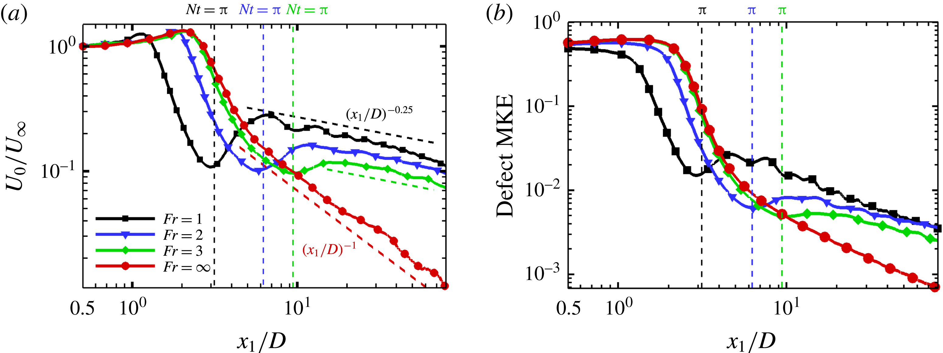
Figure 7(a) compares the evolution among the different cases of the mean defect velocity at the centreline,
 $U_{0}=U_{\infty }-\langle U_{1}\rangle _{c}$
, where
 $U_{\infty }$
is the free-stream velocity and
 $\langle U_{1}\rangle _{c}$
is the centreline streamwise mean velocity. The unstratified wake exhibits a monotone decay of the defect velocity,
 $U_{0}$
, after the recirculation region. In the near-wake subregion that extends from the end of the recirculation region up to
 $Nt\approx \unicode[STIX]{x03C0}$
, the stratified wakes also exhibit a decrease of
 $U_{0}$
with a rate that is similar to that in the unstratified case. Although
 $U_{0}$
at
 $Nt=\unicode[STIX]{x03C0}$
in the
 $Fr=3$
case is similar to that of the unstratified case, the
 $Fr=1$
and 2 wakes have significantly smaller
 $U_{0}$
at
 $Nt=\unicode[STIX]{x03C0}$
because the significantly shorter recirculation region in these wakes leads to a longer time interval for the wake deficit to decay. At
 $Nt=\unicode[STIX]{x03C0}$
, as shown by the corresponding dotted lines in figure 7(a), we find that for
 $Fr=1,2$
and 3, the defect velocity achieves a local minimum. After
 $Nt\approx \unicode[STIX]{x03C0}$
,
 $U_{0}$
starts increasing in the stratified cases. The acceleration of
 $U_{0}$
lasts until
 $Nt=\{2\unicode[STIX]{x03C0},2\unicode[STIX]{x03C0},5\}$
for the cases with
 $Fr=\{1,2,3\}$
. The increase of
 $U_{0}$
during
 $\unicode[STIX]{x03C0}<Nt<2\unicode[STIX]{x03C0}$
is prominent at
 $Fr=1$
, but becomes less so with increasing
 $Fr$
. The experiments of Bonnier & Eiff (Reference Bonnier and Eiff2002) also show a local minimum of
 $U_{0}$
followed by an abrupt increase. For
 $Fr=\{1.5,3,5\}$
and
 $Re=\{3400,6900,11\,500\}$
, the increase of
 $U_{0}$
commenced at
 $Nt=\{3,2.3,1.8\}$
and lasted until
 $Nt=\{9,7,5\}$
in their experiments. The amplitude of the increase of
 $U_{0}$
is reduced with increasing
 $Fr$
in the laboratory experiment as in our simulation.
(a) Defect velocity,
 $U_{0}$
, at the centreline (
 $x_{2}=0$
and
 $x_{3}=0$
), (b) integrated defect mean kinetic energy (MKE).

The decrease/increase of defect velocity before/after
 $Nt=\unicode[STIX]{x03C0}$
occurs because of the imprint of the steady lee wave pattern, which has a wavelength of
 $2\unicode[STIX]{x03C0}U/N$
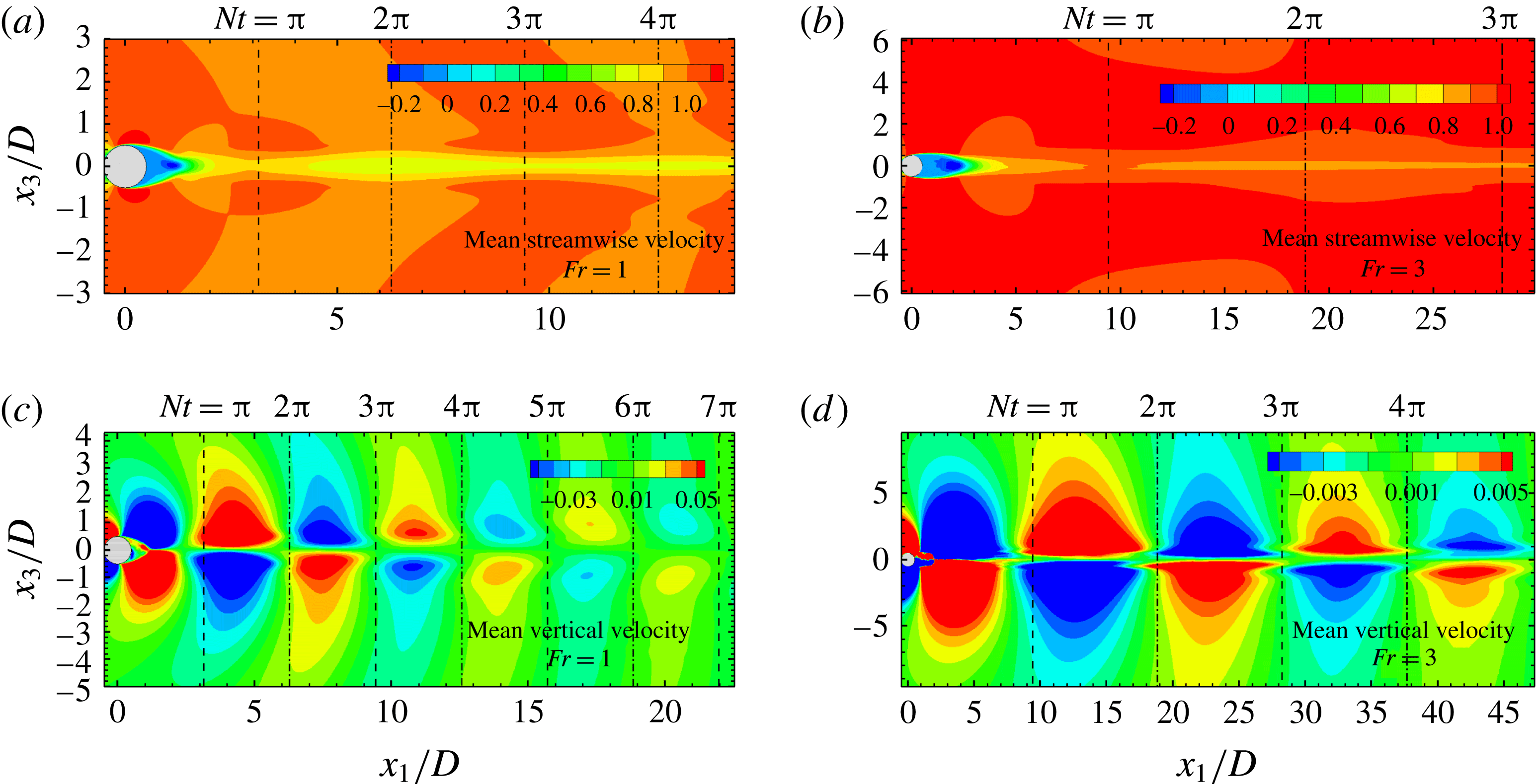
(Hunt & Snyder Reference Hunt and Snyder1980), on the stratified wake as explained below. Figure 8(a,b) presents the streamwise mean velocity
 $\langle U_{1}\rangle$
on the vertical
 $(x_{1}{-}x_{3})$
centre plane for
 $Fr=1$
and 3, respectively. It can be seen from figure 8(a) that
 $\langle U_{1}\rangle$
exhibits a non-monotone behaviour at the centreline: it increases from
 $x_{1}/D\approx 1$
up to
 $x_{1}/D\approx \unicode[STIX]{x03C0}$
, equivalently
 $Nt=\unicode[STIX]{x03C0}$
and then decreases up to the location of
 $Nt=2\unicode[STIX]{x03C0}$
. The velocity contour in the central region of the wake in figure 8(a) shows a contraction in its vertical thickness until
 $Nt=\unicode[STIX]{x03C0}$
followed by an expansion. The contraction and expansion of this central wake region repeats between
 $2\unicode[STIX]{x03C0},4\unicode[STIX]{x03C0}$
and beyond with decreasing amplitude. A similar contraction/expansion is also observed at
 $Fr=3$
for the same
 $Nt$
ranges as shown in figure 8(b). Thus, in both
 $Fr=1$
and 3 wakes,
 $Nt\in [\unicode[STIX]{x03C0},2\unicode[STIX]{x03C0}]$
exhibits a decrease in mean velocity, equivalently an increase in mean defect velocity, as was noted as a wake contraction region with accelerated defect velocity by Bonnier & Eiff (Reference Bonnier and Eiff2002) and also present in the simulations as was shown in figure 7(a). However, we note that the decrease in a characteristic vertical thickness occurs prior to the wake defect acceleration. Furthermore, the variation of the thickness of the central high-defect velocity region is oscillatory and is an effect of the body-generated lee waves on the wake of the sphere. The background signature of the lee waves is clearly visible in figure 8(a,b), particularly for the
 $Fr=1$
flow. For the
 $Fr=3$
case, the lee waves generated by the body are weak. To further clarify the lee wave effect, contours of mean vertical velocity,
 $\langle U_{3}\rangle$
, are shown in figure 8(c,d). From the edge of the sphere until
 $Nt\approx \unicode[STIX]{x03C0}$
, the sign of
 $\langle U_{3}\rangle$
shows a pattern of mean fluid convergence towards the centreline whereas, for
 $Nt\in [\unicode[STIX]{x03C0},2\unicode[STIX]{x03C0}]$
, there is a pattern of fluid divergence, thereby corroborating the fact that the vertical contraction and expansion of the high-deficit velocity region is an imprint of the body-generated lee waves. This periodic contraction–expansion behaviour in moderate-
 $Fr$
wakes occurs at intervals of
 $Nt\approx \unicode[STIX]{x03C0}$
, which coincides with the half-wavelength of the lee waves.
Contours of mean velocity on the vertical centre plane. (a,c) Corresponds to
 $Fr=1$
and (b,d) to
 $Fr=3$
. The streamwise velocity component is shown in (a,b), while the vertical component is shown in (c,d). The colour bar in (c,d) has been saturated to emphasize the lee wave pattern.

At the end of the region of vertical contraction, the defect velocity for the stratified cases starts decaying again as shown in figure 7(a). The rate of decay follows a
 $(x_{1}/D)^{-0.25}$
law for the stratified wakes as in the NEQ regime reported by Spedding (Reference Spedding1997) where
 $U_{0}$
was found to satisfy a
 $(x_{1}/D)^{-0.25}$
power law for wakes with
 $Fr\geqslant 5$
. The present simulations suggest that the power law is applicable to lower-stratification wakes too with
 $Fr$
going down to unity.
Stratification prolongs the lifetime of the entire wake deficit, not just the centreline value,
 $U_{0}$
. The streamwise evolution of the deficit mean kinetic energy (MKE) integrated over a
 $x_{2}{-}x_{3}$
cross-section is plotted in figure 7(b). High stratification (low
 $Fr$
) systematically increases the deficit MKE in the NEQ regime.
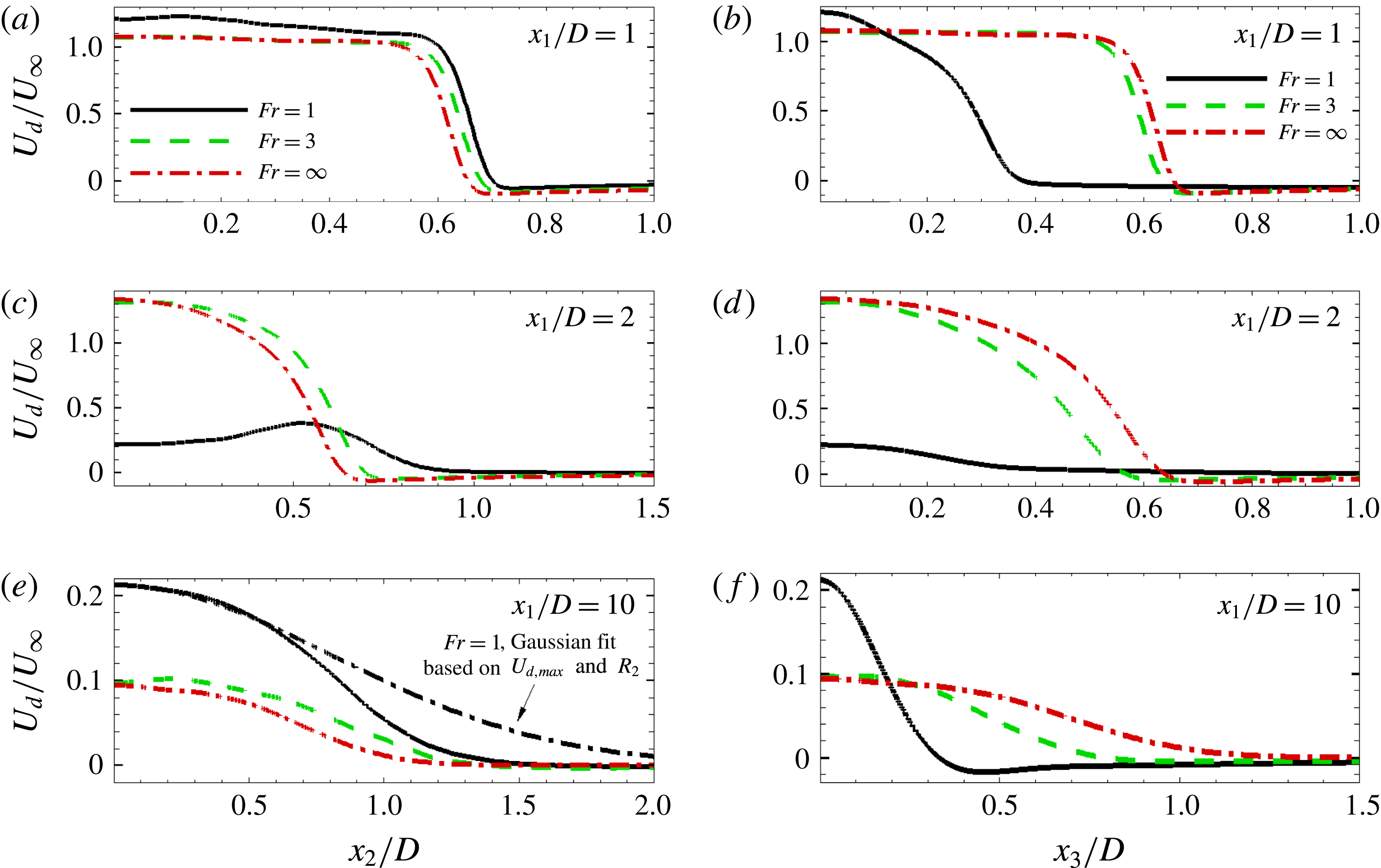
The profiles of defect velocity,
 $U_{d}=U_{\infty }-\langle U_{1}\rangle$
, in the spanwise and the vertical directions are shown in figures 9(a) and 9(b), respectively. The anisotropy between spanwise and vertical distribution of
 $U_{d}$
is significant in the
 $Fr=1$
wake but less so in the
 $Fr=3$
wake. At
 $x_{1}/D=1$
, the vertical profile of defect velocity in the
 $Fr=1$
wake shows a suppression of
 $U_{d}$
in comparison to the unstratified case because buoyancy curves the flow towards the centreline bringing in high momentum fluid. At
 $Fr=3$
, the buoyancy effect on the near wake is weaker. Notice however that although the defect velocity for
 $Fr=3$
is similar in shape to
 $Fr=\infty$
in the near wake, the effect of buoyancy is unmistakable: the velocity profile exhibits expansion and suppression of its thickness in the horizontal and vertical directions, respectively, as compared to
 $Fr=\infty$
. Further downstream at
 $x_{1}/D=10$
, the ordering of
 $U_{d}$
between the cases changes with the
 $Fr=1$
wake having a higher value of
 $U_{d}$
relative to
 $Fr=\infty$
. The reason is that the defect velocity in the
 $Fr=1$
case does not decrease relative to its value at
 $x_{1}/D=2$
as much as the unstratified case because the
 $Fr=1$
wake is already in the NEQ regime. A Gaussian function, calculated using the maximum
 $U_{d}/U_{\infty }$
and
 $R_{2}$
at the location
 $x_{1}/D=10$
, is also shown in figure 9(e). This comparison illustrates the departure of the profiles of the streamwise defect velocity from the often-assumed Gaussian.
Profiles of streamwise defect velocity for the different
 $Fr$
wakes at various
 $x_{1}/D$
locations: (a,c,e) spanwise variation and (b,d,f) vertical variation.

The balance of defect mean kinetic energy,
 $\mathit{MKE}=0.5\ast ((U_{\infty }-\langle U_{1}\rangle )^{2}+\langle U_{2}\rangle ^{2}+\langle U_{3}\rangle ^{2})$
, where
 $\langle U_{1}\rangle$
,
 $\langle U_{2}\rangle$
and
 $\langle U_{1}\rangle$
are the streamwise, horizontal and vertical mean velocities, can help better understand wake dynamics in a stratified medium. Consider the defect MKE integrated over the cross-sectional area whose evolution was shown in figure 7(b). The area-integrated turbulent production,
 $P=-\langle u_{i}^{\prime }u_{j}^{\prime }\rangle \unicode[STIX]{x2202}\langle u_{i}\rangle /\unicode[STIX]{x2202}x_{j}$
, is the primary term that is responsible for the change in defect MKE (as a function of time in the temporal model and as a function of streamwise distance in the spatial model), with the viscous dissipation of the mean flow playing a secondary role as long as turbulence is present. The entrainment into the wake brings in free-stream fluid with zero defect velocity and therefore does not contribute to the balance.
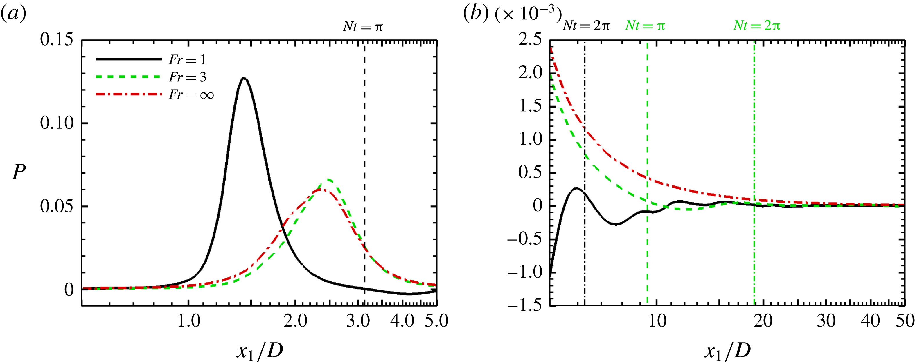
Figure 10 shows the streamwise evolution of
 $P$
integrated over the
 $x_{2}{-}x_{3}$
cross-section. At
 $0.5<x_{1}/D<\unicode[STIX]{x03C0}$
, the integrated production term is positive for
 $Fr=1$
which signifies conversion to turbulence, resulting in the streamwise decrease of area-integrated defect MKE. However, the area-integrated
 $P$
is negative over
 $\unicode[STIX]{x03C0}<x_{1}/D<2\unicode[STIX]{x03C0}$
, leading to a period of increase in the mean defect velocity as observed in figure 7. A similar period of negative integrated
 $P$
is also observed for the
 $Fr=3$
wake. The integrated
 $P$
for
 $Fr=\infty$
always remains positive, thereby leading to a monotonic decay of the mean defect velocity. Integrated
 $P$
is smaller in the stratified wakes and, therefore, the defect MKE is correspondingly larger in the presence of stratification.
Comparison of the integrated turbulent production,
 $P$
, among the different wakes: (a)
 $0.5<x_{1}/D<5$
and (b)
 $5<x_{1}/D<50$
.

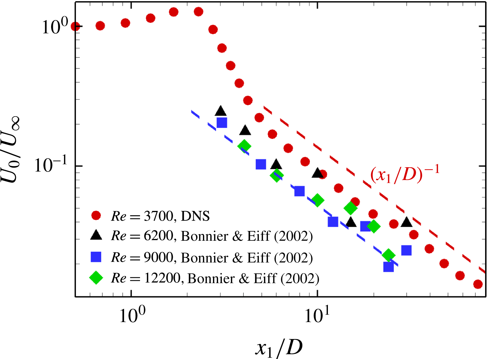
Bonnier & Eiff (Reference Bonnier and Eiff2002) measured the evolution of the centreline defect velocity,
 $U_{0}$
, in unstratified wakes and found that, for
 $2<x_{1}/D<30$
, there is a power law of
 $U_{0}\propto (x_{1}/D)^{\unicode[STIX]{x1D6FC}}$
, where
 $\unicode[STIX]{x1D6FC}\in [-0.9,-1]$
. The defect velocity in our unstratified wake simulation approximately follows a power law with
 $\unicode[STIX]{x1D6FC}=-1$
for
 $5<x_{1}/D<80$
as shown in figure 11. Chen, Gibson & Lin (Reference Chen, Gibson and Lin1968) found the value of
 $\unicode[STIX]{x1D6FC}$
to be
 $-0.85$
for
 $1.5<x_{1}/D<60$
, whereas Uberoi & Freymuth (Reference Uberoi and Freymuth1970) and Bevilaqua & Lykoudis (Reference Bevilaqua and Lykoudis1978) measured lower values of
 $\unicode[STIX]{x1D6FC}\approx -0.67$
(recall, the classical self-similarity value is
 $\unicode[STIX]{x1D6FC}=2/3$
), in the range
 $50<x_{1}/D<300$
and
 $10<x_{1}/D<100$
, respectively. The presence of the
 $(x_{1}/D)^{-1}$
scaling of the centreline defect velocity in the present unstratified axisymmetric wake may be a low-
 $Re$
regime for the scaling of the dissipation (George Reference George, George and Arndt1989) or could be attributed to the non-equilibrium turbulence dissipation law given by Nedić, Vassilicos & Ganapathisubramani (Reference Nedić, Vassilicos and Ganapathisubramani2013) and Dairay, Obligado & Vassilicos (Reference Dairay, Obligado and Vassilicos2015) that does not require low
 $Re$
. According to the non-equilibrium dissipation law,
 $\unicode[STIX]{x1D700}$
depends on the characteristic length scale and relative velocity of the wake generator as well as the local scales for turbulent kinetic energy and wake width. Given the focus of the present paper on stratification effects and the moderate
 $Re$
of the present DNS, we defer further discussion of the power-law scaling to future work that includes simulations at higher
 $Re$
.
Evolution of the centreline defect velocity in the unstratified wake: comparison of present DNS result with experiments of Bonnier & Eiff (Reference Bonnier and Eiff2002).

(a) Horizontal wake thickness
 $R_{2}$
and (b) vertical wake thickness
 $R_{3}$
for various
 $Fr$
. Note that the vertical scale in (b) is different than in (a).

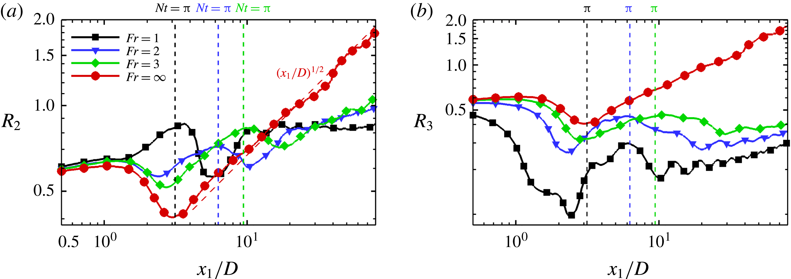
To quantify the thickness of the wake for the stratified cases, half-widths in the horizontal (
 $R_{2}$
) and vertical direction (
 $R_{3}$
) are presented in figures 12(a) and 12(b), respectively. The half-width is defined as the radial distance to the location where the defect velocity reduces to half of its value at the centreline.
For the unstratified case, azimuthal averaging is performed in addition to time averaging for calculating the half-width. Near the body and in the unstratified case, the half-width of the velocity profile initially decreases in the recirculation zone and then increases as the wake profile forms and progressively thickens by turbulent entrainment. This behaviour holds qualitatively for the
 $Fr=2$
and 3 cases too. The unstratified axisymmetric wake thickness evolves as
 $(x_{1}/D)^{1/2}$
consistent with the
 $(x_{1}/D)^{-1}$
scaling of the centreline defect velocity. Buoyancy eventually reduces the horizontal thickness of the stratified wakes relative to the unstratified counterpart. The recirculation region progressively shortens with increasing
 $Fr$
and the shortening is anisotropic. The separated boundary layer in the
 $Fr=1$
case plunges inward in the vertical plane owing to buoyancy and the defect velocity at the centreline drops significantly within a short distance from the sphere. The horizontal half-width does not exhibit an initial decrease in the
 $Fr=1$
wake as can also be surmised by comparing the
 $x_{2}$
-profiles of
 $U_{0}$
in figure 9 between the
 $x_{1}/d=1$
and
 $x_{1}/d=2$
locations. However, comparison of the
 $x_{3}$
profiles between
 $x_{1}/d=1$
and
 $x_{1}/d=2$
suggests a decrease in
 $R_{3}$
for the
 $Fr=1$
wake which is confirmed by figure 12(b). The
 $Fr=1$
wake shows a substantial decrease in
 $R_{2}$
between
 $Nt=\unicode[STIX]{x03C0}$
and
 $2\unicode[STIX]{x03C0}$
. This is because, as previously discussed, there is a prominent increase in centreline defect velocity,
 $U_{0}$
, during this period owing to the lee wave while the velocity further away from the body is less affected. The consequent change of shape of the profile directly results in a decrease in the horizontal half-width. The
 $Fr=2$
and 3 wakes also show a decrease of
 $R_{2}$
during this period. The vertical thickness,
 $R_{3}$
, of the stratified wakes is generally smaller than
 $R_{2}$
.
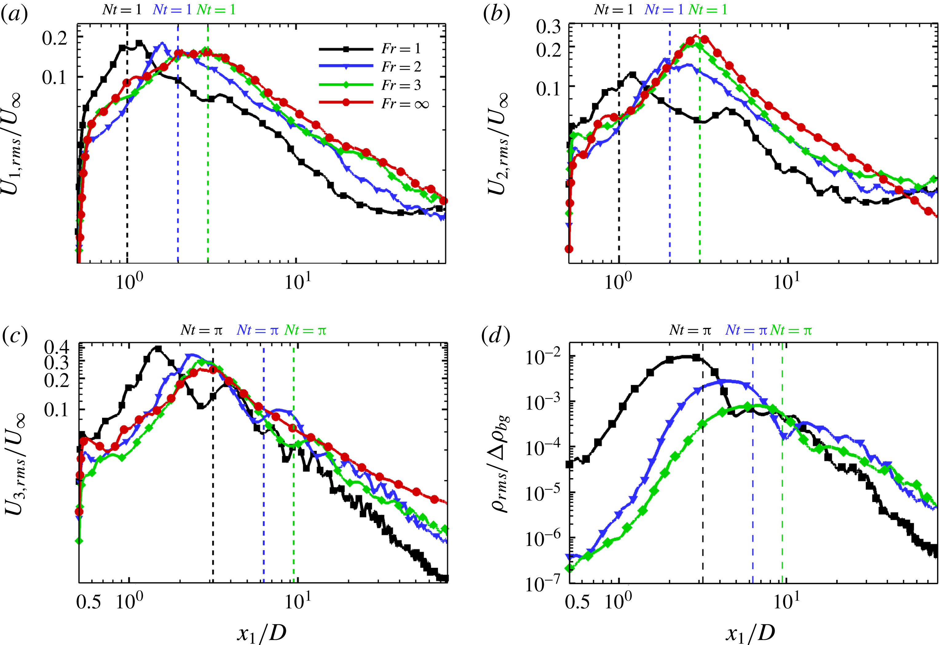
Behaviour of r.m.s. turbulence quantities at the centreline: (a) streamwise velocity, (b) horizontal velocity, (c) vertical velocity and (d) density deviation.

5 Turbulence levels
Buoyancy affects turbulence fluctuations differently near the body relative to locations further away. The effect is also anisotropic as can be seen from figure 13 that shows the streamwise evolution at the centreline of the r.m.s. of all velocity components, normalized with the body relative velocity
 $U$
, and the density r.m.s., normalized with
 $\unicode[STIX]{x0394}\unicode[STIX]{x1D70C}_{bg}=D(\unicode[STIX]{x2202}\unicode[STIX]{x1D70C}/\unicode[STIX]{x2202}z)_{bg}$
. We elaborate below.
Notably, the peak value of the streamwise component,
 $u_{1,rms}$
(figure 13
a) occurs at a similar buoyancy time,
 $Nt\approx 1$
, in all stratified cases. Also, the peak values achieved at the stronger stratification of
 $Fr=1$
and 2 are similar and are
 ${\approx}10\,\%$
higher than the values at
 $Fr=3$
and the non-stratified case. The inward vertical motion behind the sphere induced by the restoring force of buoyancy brings in high momentum fluid towards the centreline, thereby increasing
 $u_{1,rms}$
for the
 $Fr=1$
and 2 wakes. After
 $Nt\approx 1$
,
 $u_{1,rms}$
decays for all the stratified cases. The value of
 $u_{1,rms}$
for the
 $Fr=1$
case becomes lower than in the other cases for the same
 $x_{1}/D$
location. However, the decay of
 $u_{1,rms}$
for
 $Fr=1$
slows down at
 $x_{1}/D\sim 20$
and reaches a plateau beyond that location whereas the other cases continue decaying at a similar rate. Figure 13(b) presents the evolution of the spanwise (horizontal) r.m.s. velocity at the centreline for the different cases.
 $u_{2,rms}$
for all the stratified cases once again peaks at
 $Nt\approx 1$
, however the peak values decrease with increasing stratification unlike
 $u_{1,rms}$
. The maximum value of
 $u_{2,rms}$
for
 $Fr=1$
is
 ${\approx}50\,\%$
, for
 $Fr=2$
is
 ${\approx}33\,\%$
and
 $Fr=3$
is
 ${\approx}12.5\,\%$
less than the peak value of
 $u_{2,rms}$
for the non-stratified case. The decay of centreline
 $u_{2,rms}$
for the stratified cases slows down after
 $x_{1}/D\sim 9$
as compared to the continuous decay in the unstratified case. By
 $x_{1}/D=10$
, there are significant differences in the streamwise r.m.s. profiles among the
 $Fr=1,3$
and
 $\infty$
wakes.
The evolution of the centreline vertical r.m.s. velocity (figure 13
c) shows that, similar to the streamwise component, the maximum value of
 $u_{3,rms}$
is higher in the stratified wakes:
 $Fr=1$
has
 ${\approx}38\,\%$
,
 $Fr=2$
has
 ${\approx}29\,\%$
and
 $Fr=3$
has
 ${\approx}20\,\%$
higher values relative to the non-stratified case. The increase in the vertical and streamwise fluctuation is due to the unsteady inward plunging of the flow in the vertical plane after separation that is induced by buoyancy. Notice that the frequency of oscillations is higher as the background buoyancy frequency increases. With increasing stratification, the decay of
 $u_{3,rms}$
becomes faster than in the unstratified case. Also,
 $u_{3,rms}$
becomes progressively smaller relative to the horizontal components showing the eventual dominance of horizontal motions as the stratified wake enters the regime of low local Froude number. The r.m.s. of the normalized density deviation at the centreline is shown in figure 13(d). It peaks shortly before
 $Nt=\unicode[STIX]{x03C0}$
followed by an oscillatory decay. The peak value is largest for the highest stratification of
 $Fr=1$
, consistent with larger vertical fluctuations in this near-body region. The subsequent decay is larger for the
 $Fr=1$
wake and eventually the ordering of
 $\unicode[STIX]{x1D70C}_{rms}/\unicode[STIX]{x0394}\unicode[STIX]{x1D70C}_{bg}$
among the
 $Fr$
cases is similar to that for
 $u_{3,rms}$
.
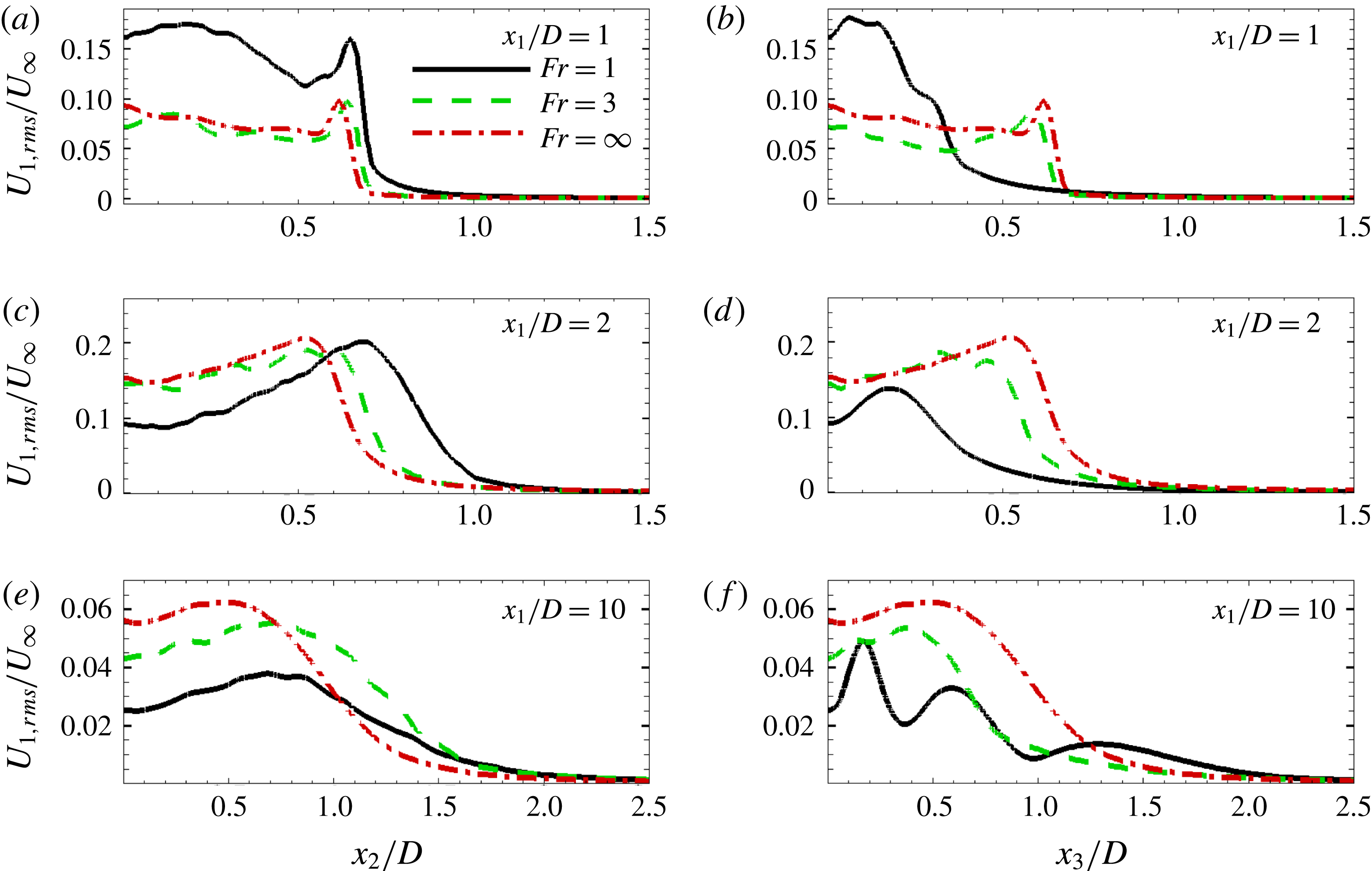
Profiles of streamwise r.m.s. velocity at different
 $x_{1}/D$
locations as a function of (a,c,e) horizontal and (b,d,f) vertical direction.

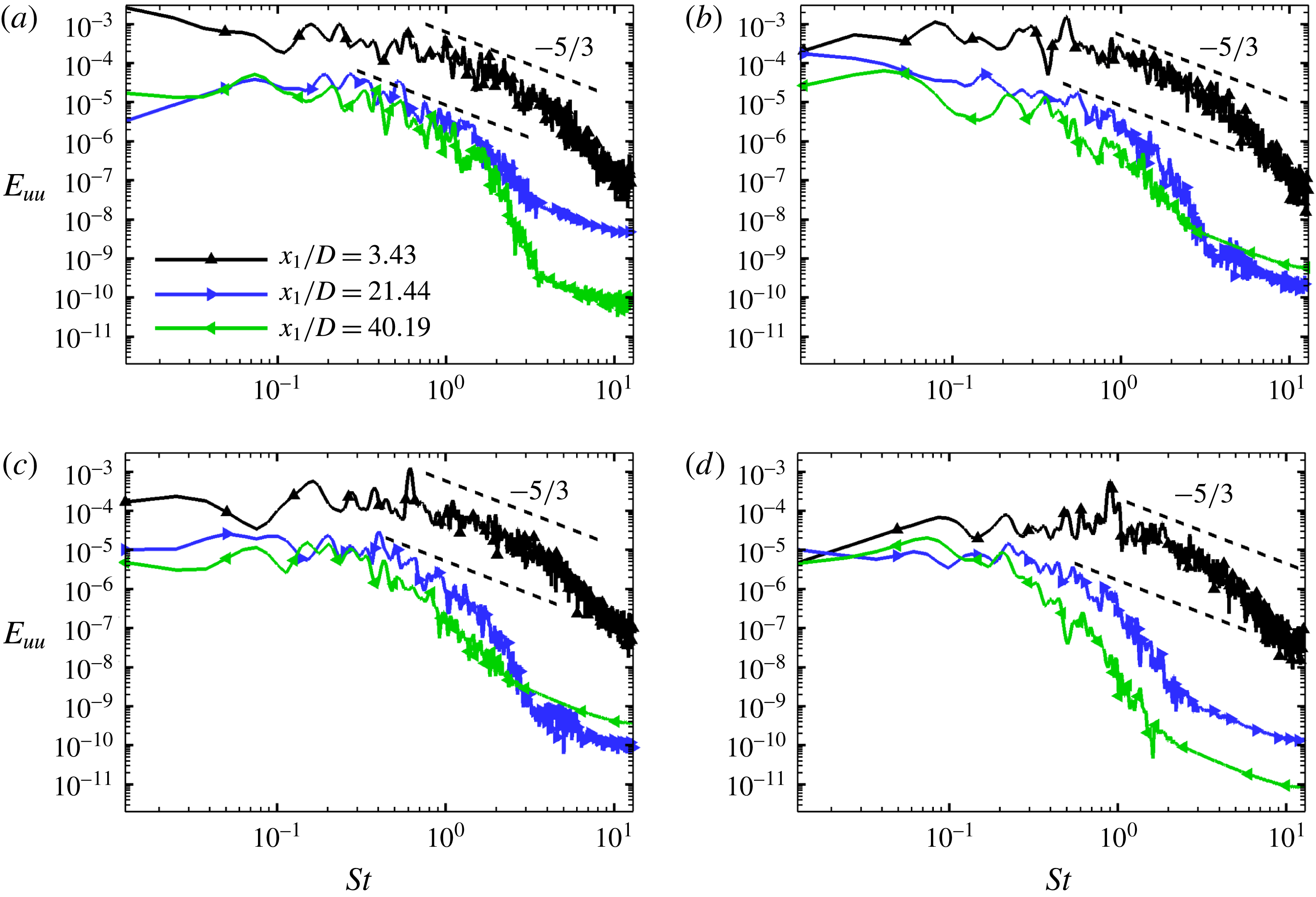
Temporal spectra of the streamwise velocity at different downstream (
 $x_{1}/D$
) locations on the centreline (
 $x_{2}/D=0,x_{3}/D=0$
) as a function of Strouhal number,
 $St=Uf/D$
: (a)
 $Fr=\infty$
, (b)
 $Fr=3$
, (c)
 $Fr=2$
and (d)
 $Fr=1$
.

The spatial variation of streamwise r.m.s. velocity is compared among cases with horizontal (spanwise) and vertical profiles shown in figures 14(a,c,e) and 14(b,d,f), respectively. Close to the body (
 $x_{1}/D=1$
), there is an outer peak corresponding to the horizontal shear layer and the
 $Fr=1$
case has higher fluctuation levels. By
 $x_{1}/D=2$
, turbulence in the
 $Fr=1$
wake exhibits significant anisotropy in its spatial variation (shorter in the vertical relative to the horizontal) that results in lower fluctuations at the centreline and along the vertical (
 $x_{3}$
) coordinate. At
 $x_{1}/D=10$
, even the
 $Fr=3$
wake exhibits spatial anisotropy. Oscillations in the vertical profile are noticeable for the
 $Fr=1$
wake at
 $x_{1}/D=10$
owing to internal waves.
6 Spectra
Figure 15(a–d) presents the
 $u_{1}$
-power spectra at different locations on the centreline for the cases simulated here. The
 $Fr=\infty$
wake has a short range of scales with a slope that is near
 $-5/3$
at
 $x_{1}/D=3.43$
and 21.44. The spectrum in the
 $Fr=3$
case also has a similar range of scales with an approximately inertial scaling at
 $x_{1}/D=3.43$
but, by
 $x_{1}/D=21.44$
, it exhibits a steeper scaling. Presumably, at the moderate
 $Re=3700$
of the present simulation, buoyancy is already able to alter the energy cascade at
 $x_{1}/D=21.44$
(
 $Nt=7.1$
). The strong stratification in the
 $Fr=1$
case eliminates any resemblance to inertial scaling in the spectra even near the body at
 $x_{1}/D=3.43$
.
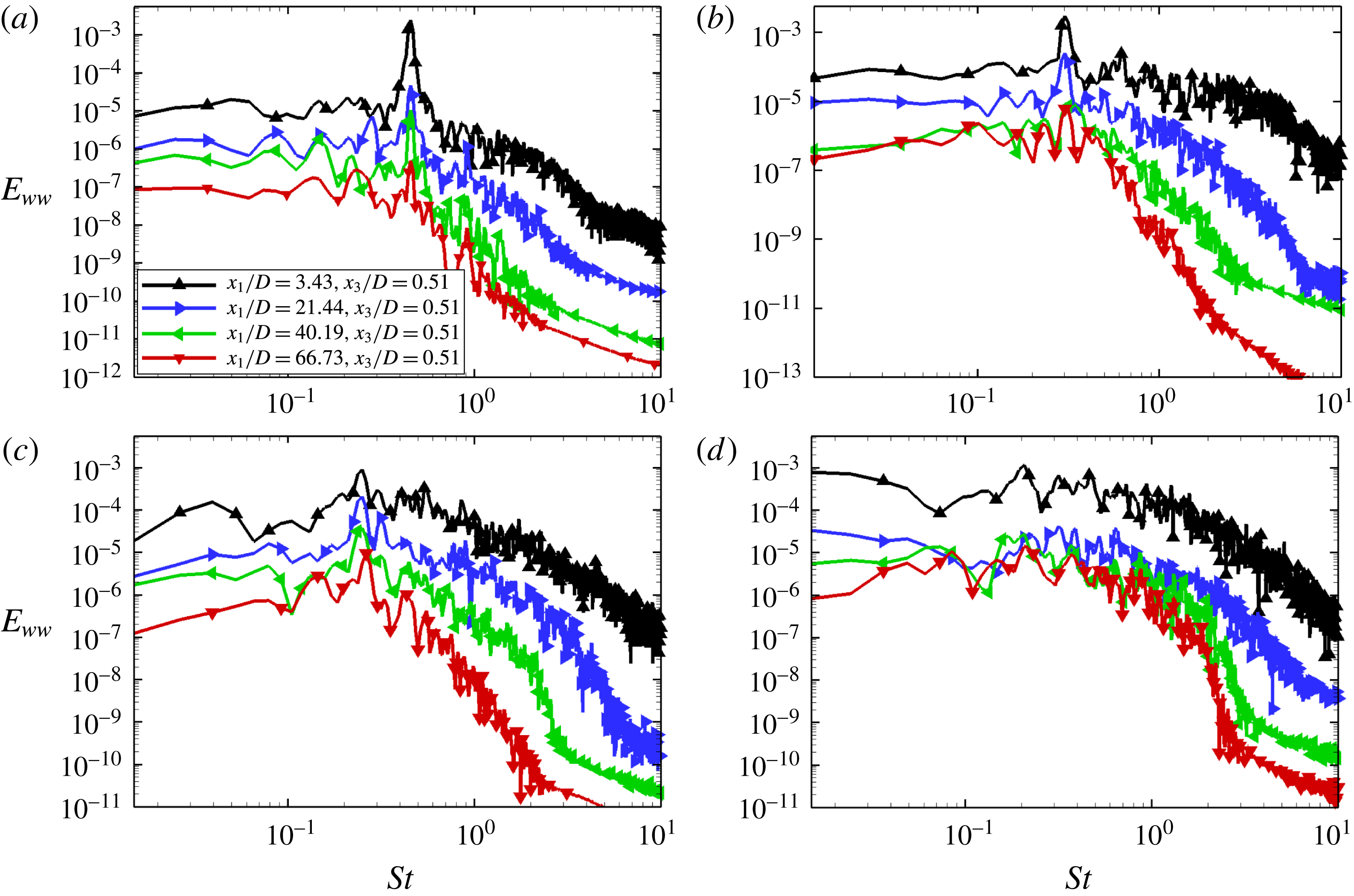
Figure 16 shows spectra of the vertical velocity at different streamwise locations on a horizontal line (
 $x_{2}=0,x_{3}=0.51$
) that is vertically offset by a distance of 0.51 from the centreline. The
 $Fr=1$
wake (figure 16
a) exhibits a discrete spectral peak at
 $St=0.456$
for all the shown downstream locations. The
 $Fr=2$
wake (figure 16
b) also exhibits a discrete spectral peak, whose characteristic frequency is 0.307. The spectra indicate that the
 $Fr=2$
wake is more energetic across scales relative to
 $Fr=1$
at the different
 $x_{1}/D$
locations. The
 $Fr=3$
wake has a characteristic frequency (
 $St=0.24$
) too but the peak is less prominent and the broadband spectrum is more energetic than in the lower-
 $Fr$
wakes. The unstratified case shows a characteristic frequency of
 $St=0.21$
near the body but it is not preserved further downstream.
Spectra of the vertical velocity at a vertical location
 $x_{3}/D=0.51$
and different downstream locations: (a)
 $Fr=1$
, (b)
 $Fr=2$
, (c)
 $Fr=3$
and (d)
 $Fr=\infty$
.

7 Turbulent kinetic energy and its budget
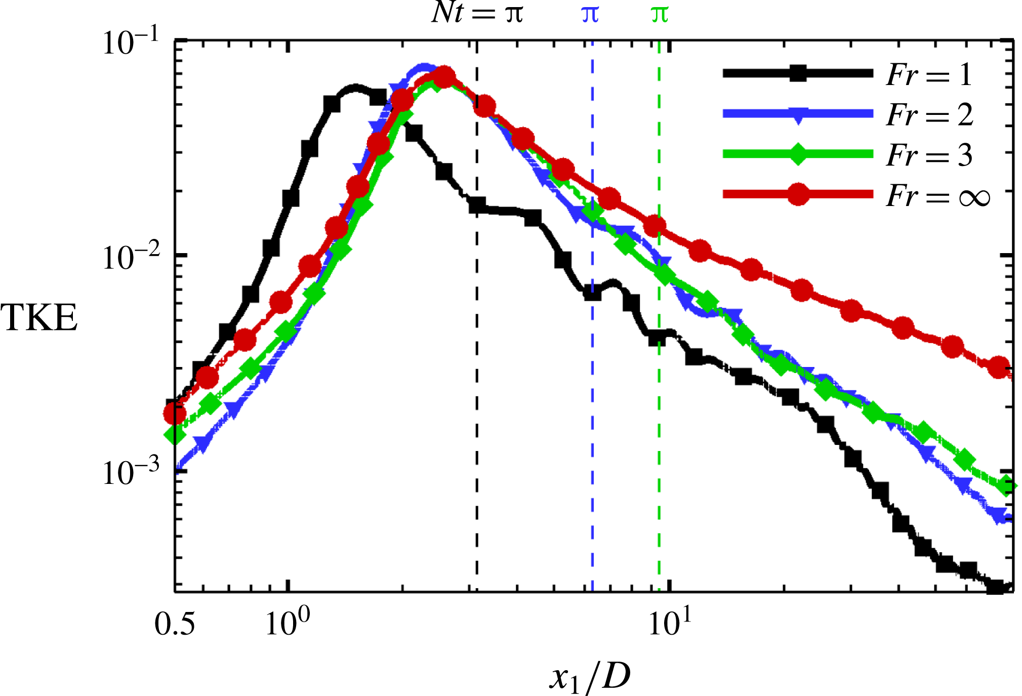
The streamwise evolution of the turbulent kinetic energy
 $\mathit{TKE}=\langle u_{i}^{\prime }u_{i}^{\prime }\rangle /2$
, integrated over the
 $x_{2}$
–
 $x_{3}$
cross-section, is shown in figure 17. The maximum of the integrated TKE has a similar magnitude among all cases, with the peaks approximately located at the end of the recirculation regime for each case. A significant departure of TKE for
 $Fr=3$
from the
 $Fr=\infty$
case can be observed at
 $x_{1}/D\approx 5$
with the point of departure moving closer to the sphere with decreasing
 $Fr$
. The
 $Fr=1$
and 2 wakes exhibit noticeable oscillations with a period of approximately
 $t=\unicode[STIX]{x03C0}/N$
, related to the lee wave imprint on the wake that was discussed earlier. The TKE budget equation at statistical steady state in the Cartesian coordinate system is given by
 $$\begin{eqnarray}0=-A+P+B-\unicode[STIX]{x1D700}-T,\end{eqnarray}$$
where
 $$\begin{eqnarray}A=\langle u_{j}\rangle \frac{\unicode[STIX]{x2202}(\mathit{TKE})}{\unicode[STIX]{x2202}x_{j}},\quad P=-\langle u_{i}^{\prime }u_{j}^{\prime }\rangle \frac{\text{d}U_{i}}{\text{d}x_{j}},\quad B=-\frac{g}{\unicode[STIX]{x1D70C}_{0}}\langle \unicode[STIX]{x1D70C}^{\prime }u_{3}^{\prime }\rangle ,\end{eqnarray}$$
are the advection, production and buoyancy flux, respectively,
 $$\begin{eqnarray}\unicode[STIX]{x1D700}=2\unicode[STIX]{x1D708}\langle s_{ij}^{\prime }s_{ij}^{\prime }\rangle ,\quad \text{with }s_{ij}^{\prime }=\frac{1}{2}\left(\frac{\unicode[STIX]{x2202}u_{i}^{\prime }}{\unicode[STIX]{x2202}x_{j}}+\frac{\unicode[STIX]{x2202}u_{j}^{\prime }}{\unicode[STIX]{x2202}x_{i}}\right),\end{eqnarray}$$
is the turbulent dissipation rate and
 $T=\unicode[STIX]{x2202}T_{i}^{\prime }/\unicode[STIX]{x2202}x_{i}$
is the transport term with
 $$\begin{eqnarray}T_{i}^{\prime }={\textstyle \frac{1}{2}}\langle u_{i}^{\prime }u_{j}^{\prime }u_{j}^{\prime }\rangle +\langle u_{i}^{\prime }p^{\prime }\rangle /\unicode[STIX]{x1D70C}_{0}-2\unicode[STIX]{x1D708}\langle u_{j}^{\prime }s_{ij}^{\prime }\rangle .\end{eqnarray}$$
The governing equations are solved on a cylindrical grid, therefore the velocities and derivatives are transformed into the Cartesian coordinate system using (2.7) and (2.8), and then the terms of the TKE budget equation are computed in Cartesian coordinates.
Streamwise variation of the area-integrated TKE for wakes at different
 $Fr$
.

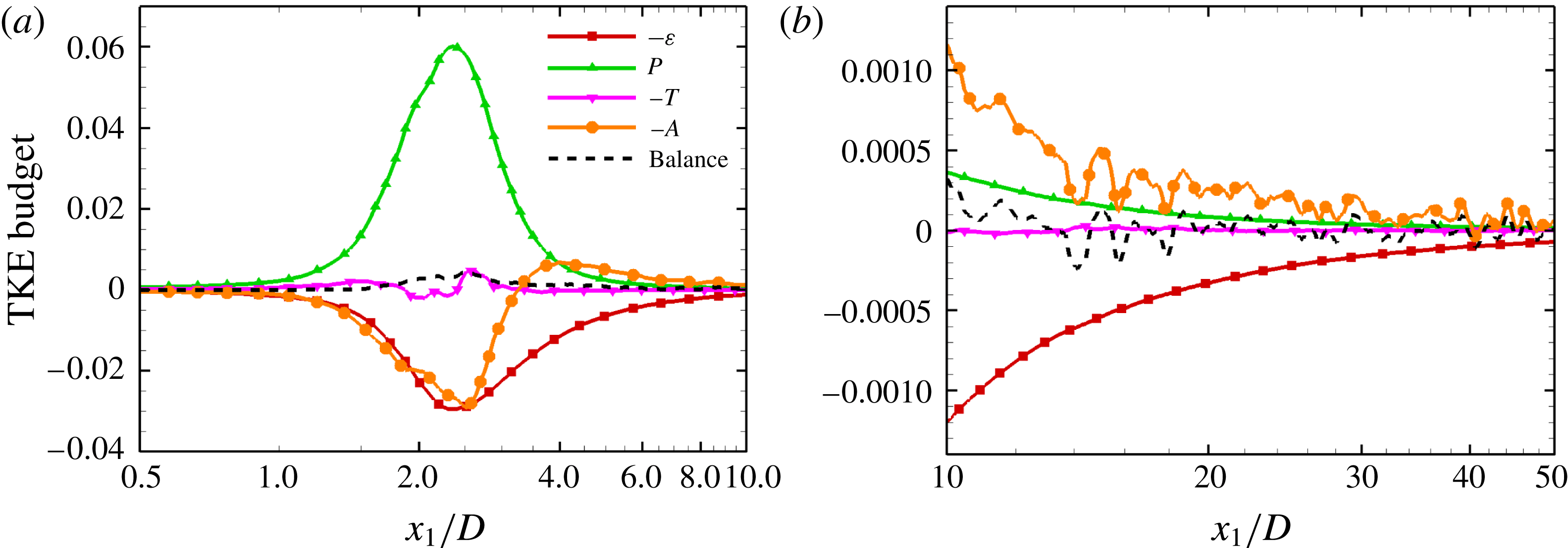
The terms in the turbulent kinetic energy budget equation for
 $Fr=\infty$
: (a)
 $0.5<x_{1}/D<10$
and (b)
 $10<x_{1}/D<50$
.

Figure 18(a,b) presents the TKE budget integrated over a circle with radius
 $3$
that fully contains the wake TKE region for the unstratified case. Near and aft of the sphere, the turbulent shear layer becomes unstable owing to Kelvin–Helmholtz billows which break down into turbulence. The separated shear layer interacts with the body and forms a turbulent recirculation zone. Turbulent production,
 $P$
, dominates in the interval
 $0.5<x_{1}/D<3.5$
, and is balanced by advection and dissipation. Notice that the production, advection and dissipation attain local maxima at
 $x_{1}/D\approx 2.4$
, close to the end of the recirculation region. Beyond
 $x_{1}/D\approx 3.5$
, dissipation becomes larger than production. Further downstream (figure 18
b), shear production becomes small and the balance is between advection and dissipation. The area-integrated transport term remains negligible throughout the evolution.
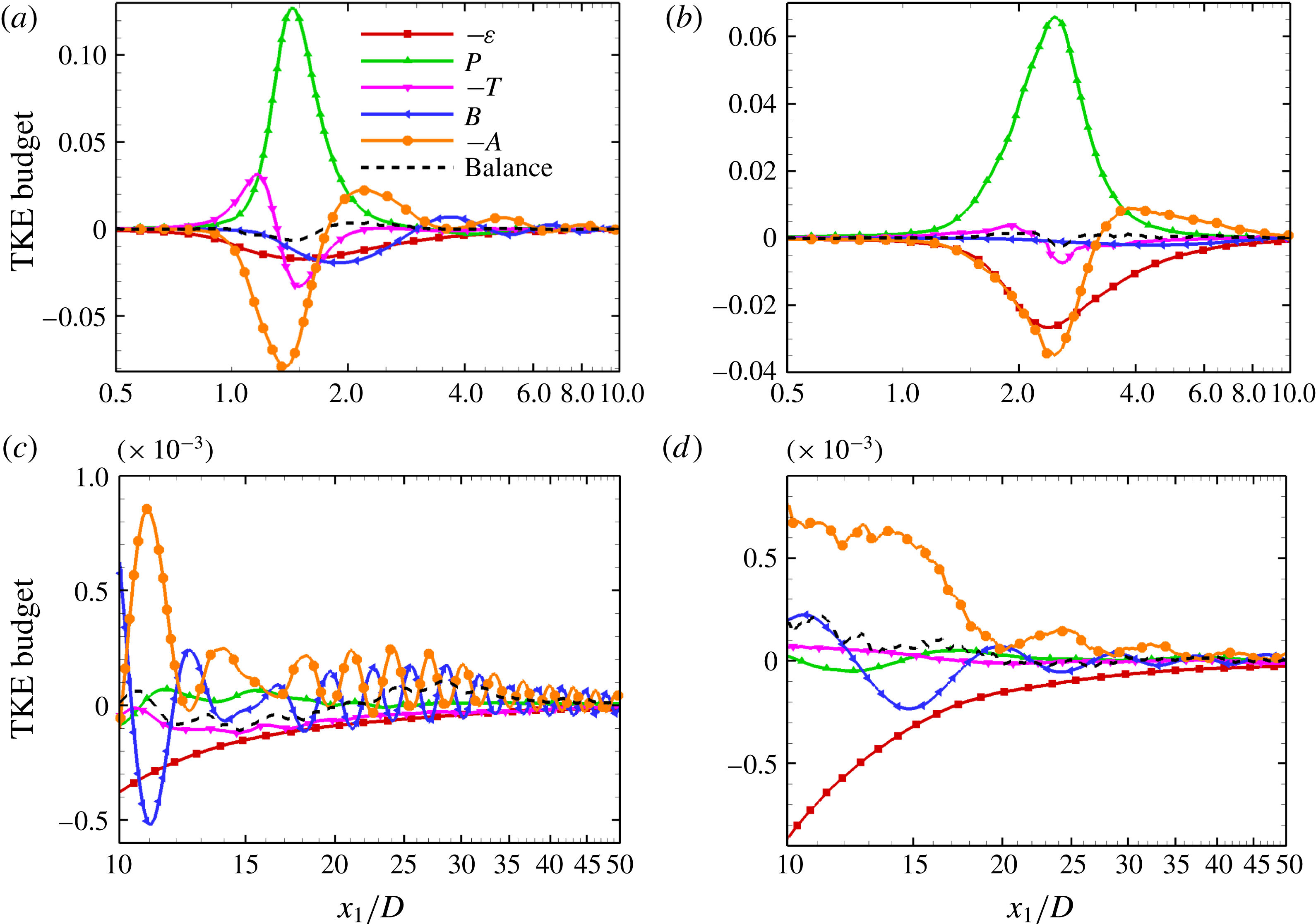
The terms in the TKE budget compared between
 $Fr=1$
(a,c) and
 $Fr=3$
(b,d).

Figure 19 compares the TKE budget between
 $Fr=1$
and 3 over different ranges of
 $x_{1}/D$
. The maximum value of turbulent production,
 $P$
, for the
 $Fr=1$
(figure 19
a) case is almost twice that at
 $Fr=3$
(figure 19
b). The sharp inward curving of the shear layer (figure 4
a) at
 $Fr=1$
brings high momentum fluid into the region behind the sphere spanning
 $0<x_{1}/D<1.5$
resulting in larger
 $P$
in that region. The transport term also acts as a source of TKE for
 $0<x_{1}/D<1.5$
. Although the production is high for
 $Fr=1$
, the dissipation,
 $\unicode[STIX]{x1D700}$
, is less than that for
 $Fr=3$
and
 $\infty$
case (figures 18
a and 19
b). A fraction of the turbulence generated by the high production for
 $Fr=1$
is carried away by internal waves, as evidenced by the negative value of the transport term (dominated by pressure transport) and the rest is dissipated via viscosity. Internal waves play a vital role in the balance as suggested by the importance of the integrated transport term. For
 $Fr=3$
, the waves are weak for the moderate-
 $Re$
wake simulated here, and the transport term is much smaller than at
 $Fr=1$
. Therefore, most of the fluctuation energy is dissipated locally by viscosity in
 $Fr=3$
wake.
The advective term remains positive until
 $x_{1}/D\approx 2$
for
 $Fr=1$
as compared to
 $x_{1}/D\approx 3.5$
for the
 $Fr=3$
and
 $\infty$
cases. We also find reversible transfer between turbulent kinetic and potential energy modes as the buoyancy flux switches signs for
 $Fr=1$
, whereas this transfer for
 $Fr=3$
within
 $0.5<x_{1}/D<10$
is small. After
 $x_{1}/D\approx 2$
, the combination of the dissipation and the buoyancy flux dominates the production term and the advective term acts as a gain. The behaviour of the TKE budget terms for
 $Fr=3$
(figure 19
b) is similar to the unstratified case within
 $0.5<x_{1}/D<10$
. The stronger effect of buoyancy for
 $Fr=1$
is evident from the dominance of local buoyancy flux within the range
 $10<x_{1}/D<50$
(figure 19
c), with advection being of the same order. The production, dissipation and the transport terms have comparable values. The transport of TKE away from the wake, owing to the propagation of internal waves, is also evident by the negative value of the transport. The
 $Fr=3$
case (figure 19
d) has comparable dissipation, advection and buoyancy flux terms with lower values of the production and transport terms.
8 Summary and conclusions
DNS of flow past a sphere at
 $Re=3700$
has been performed in the regime of moderate stratification (
 $Fr=U_{\infty }/ND=O(1)$
) for cases with
 $Fr=1,2,3$
as well as an unstratified case with
 $Fr=\infty$
. The behaviour of highly stratified wakes with
 $Fr<O(1)$
was reported previously by Pal et al. (Reference Pal, Sarkar, Posa and Balaras2016). The Navier–Stokes equations are solved on a cylindrical coordinate system and the sphere is represented using an immersed boundary method. The numerical model has been validated against previous results of unstratified flow (both laboratory and DNS studies) as well as stratified flow (laboratory study) past a sphere. The evolution of the unstratified case is simulated into the far wake up to
 $x_{1}/D=80$
as are the stratified cases. Inclusion of the sphere allows us to investigate the effect of buoyancy on the recirculation region, the near wake and the transition from the near wake to the non-equilibrium (NEQ) region. The presence of the body in our simulations has allowed new computational results that cannot be obtained by a typical temporal model, e.g. the interaction of the body-generated lee wave with the wake to increase the defect velocity relative to the unstratified case, anisotropy of near-wake turbulence levels and profiles and downstream persistence of spectral frequencies associated with vortex shedding. We also recover results obtained by previous temporal simulations of the far wake, e.g. the presence of an NEQ regime with an approximately
 $(x_{1}/D)^{-0.25}$
power law and a reduction of TKE production that diminishes the transfer of MKE to TKE, thus keeping the mean defect velocity high in stratified wakes.
The centreline mean defect velocity,
 $U_{0}$
, of the unstratified wake decays after the recirculation zone as
 $U_{0}\propto x_{1}^{-1}$
, different from the classical, self-similar scaling of
 $x_{1}^{-2/3}$
, and in agreement with the measurements of the sphere wake by Bonnier & Eiff (Reference Bonnier and Eiff2002) and other axisymmetric wakes by Nedić et al. (Reference Nedić, Vassilicos and Ganapathisubramani2013) and Dairay et al. (Reference Dairay, Obligado and Vassilicos2015). The recirculation zone shortens with increasing buoyancy owing to the plunging of the separated flow in the vertical plane brought about by the restoring force of buoyancy which tends to return displaced fluid back towards its neutral position. The recirculation region is followed by a decrease of
 $U_{0}$
with a rate that is similar to that in the unstratified case until
 $Nt=\unicode[STIX]{x03C0}$
after which
 $U_{0}$
increases with increasing
 $x_{1}/D$
. The period of increasing
 $U_{0}$
ends at
 $Nt\approx 2\unicode[STIX]{x03C0}$
, beyond which the wake shows the
 $U_{0}\propto (x_{1}/D)^{-.25}$
power-law characteristic of the NEQ regime. Bonnier & Eiff (Reference Bonnier and Eiff2002) also identified a phase of acceleration of
 $U_{0}$
in their laboratory experiments and speculated that the energy source could be the collapse of three-dimensional turbulent motions or the release of the potential energy stored in density fluctuations of the near wake. We find that the increase of
 $U_{0}$
is actually the half-cycle of an decaying oscillatory modulation of
 $U_{0}$
with period
 $Nt=2\unicode[STIX]{x03C0}$
that is the imprint of a steady lee wave pattern. It is worth noting that a turbulence collapse or release of potential energy in the wake would increase the mean fluid velocity and decrease the defect velocity,
 $U_{0}$
, instead of the observed increase of
 $U_{0}$
. The lee wave leads to a periodic pattern of vertical flow convergence and divergence at the centreline, thus modulating the thickness and streamwise velocity of the central wake region.
Spedding (Reference Spedding1997) reports
 $Nt\approx 2$
as the beginning of the NEQ regime in stratified wakes with
 $Fr>O(1)$
. In the
 $Fr=O(1)$
wakes examined here,
 $Nt\approx \unicode[STIX]{x03C0}$
marks the point where the wake deficit velocity increases and the transition into the
 $NEQ$
regime commences. The decay of
 $U_{0}$
slows down significantly in the NEQ regime with
 $U_{0}\propto (x_{1}/D)^{-0.25}$
for all the simulated stratified cases. Thus, the
 $(x_{1}/D)^{-0.25}$
scaling seen by Spedding (Reference Spedding1997) for
 $Fr>5$
wakes is applicable to lower stratifications down to
 $Fr=1$
.
 $U_{0}$
is larger in stratified wakes at the beginning of the NEQ regime because of the wake contraction/expansion induced by the lee wave. During the NEQ regime, the mean deficit of the stratified wakes becomes progressively larger relative to their unstratified counterpart and, by
 $x/d=80$
, the
 $Fr=3$
wake has an order of magnitude larger
 $U_{0}$
and defect MKE. The longer life time of the mean stratified wake is facilitated in the NEQ regime because buoyancy reduces the loss to turbulence, i.e. turbulent production,
 $P$
, is severely reduced, e.g.
 $P$
crosses zero at
 $Nt=2\unicode[STIX]{x03C0}$
. Furthermore, the flow organizes into coherent horizontal motions.
Buoyancy changes TKE levels and introduces significant anisotropy in the fluctuations, both among vertical and horizontal velocity components and in their spatial organization. Therefore, the choice of initial fluctuation profiles for a temporal model will present a challenge for wakes with stratification levels equal or more than those examined here. Near the body, TKE is larger at
 $Fr=1$
but, by
 $Nt=2$
, becomes significantly smaller than at
 $Fr=\infty$
. The vertical component decays faster than the horizontal components and has a discrete peak in its spectrum near the body that remains prominent at downstream locations. The spatial profiles of the r.m.s. turbulence are substantially different relative to the unstratified case, e.g. at
 $x_{1}/D=10$
, the horizontal width of the streamwise r.m.s. profile in the
 $Fr=3$
wake is larger while the vertical width is smaller than in the
 $Fr=\infty$
wake.
The TKE budget terms, integrated over an area that encloses the wake, show a good balance for all cases owing to the high resolution that is employed. In the unstratified wake, production is the dominant term until
 $x_{1}/D=3$
, and is balanced by dissipation and advection. Further downstream, production becomes increasingly less important (by
 $x_{1}/D\approx 10$
, production is one third of the dissipation) and the balance shifts to one between advection and dissipation. The dominance of advection over production as the source of TKE is an important distinction between wakes and other shear flows which contributes to the long memory of near-body turbulence in the wake. Buoyancy and transport through the pressure–velocity correlation contribute to the balance in the stratified flows, from near the body at
 $Fr=1$
and from
 $x_{1}/D\approx 9$
(
 $Nt\approx 3$
) at
 $Fr=3$
. The
 $Fr=1$
case has a prominent internal wave signature in visualizations and, correspondingly, the pressure transport is also important displaying an oscillatory behaviour near the body and then, further downstream, acting as a consistent sink of TKE.
Internal waves are an important constituent of fluctuating motion in stratified flows past bodies. Quantification of the properties of internal waves and their variation as a function of
 $Fr$
is the subject of ongoing work. The present results have been obtained at a moderate
 $Re$
and moderate
 $Fr$
. The near wake operates in the stratified turbulence regime of
 $Fr\sim O(1)$
and high buoyancy Reynolds number. However, the strongly stratified intermediate wake at a sphere
 $Re=3700$
is not at a buoyancy Reynolds number above unity and, therefore, the strongly stratified turbulence regime (e.g. see review by Riley and Lindborg in Davidson, Kaneda & Sreenivasan Reference Davidson, Kaneda and Sreenivasan2013) is not reached. Simulations at higher
 $Re$
will be necessary to ascertain the
 $Re$
effect on intermediate-wake behaviour and, with higher
 $Fr$
simulations, this work can be extended to low-stratification wakes.
Acknowledgements
We gratefully acknowledge the support of ONR grant no. N00014-15-1-2718, program manager Dr T. Fu. Computational resources were provided by the Department of Defense High Performance Computing Modernization Program.