1. Introduction

An important recent development in the naturalistic study of communication is the systematic investigation of simple, computationally tractable models. Such models are severely idealized in many respects, but there are invaluable gains in the explicitness and rigor of the results obtained by working on them, alongside the familiar approach of engaging in informal discussion of more realistic examples. Some areas of concern to philosophers that this research program has already shed light on are the difference between assertions (indicatives) and directives (imperatives) (Huttegger Reference Huttegger2007; Zollman Reference Zollman2011), signaling in social dilemmas (Wagner Reference Wagner2015), deception (Zollman, Bergstrom, and Huttegger Reference Zollman, Bergstrom and Huttegger2013; Martínez Reference Martínez2015), and vagueness (O’Connor Reference O’Connor2014).

Formulating the problem of communication in a way that makes it amenable to a rigorous treatment of this kind is in itself a major philosophical contribution. Most of the work cited above is based on Lewis’s (Reference Lewis1969/2002) model of signaling. In this model a sender (or, for Lewis, ‘communicator’) sends messages to a receiver (or, for Lewis, an ‘audience’), and both parties receive a payoff that depends on the state the world is in when the message is sent and the act performed by the receiver in response. (In this article we focus on so-called cheap talk games, in which payoffs do not depend on the type of message sent.) The message sent by the sender on a given occasion is decided by a sender’s strategy: a function that takes states (i.e., members of a set S of mutually exclusive and jointly exhaustive ways the world can be) to a probability distribution over the set M of possible messages. The act performed by the receiver is decided by a receiver’s strategy: a function that takes each member of M to a probability distribution over the set A of possible acts. A signaling game is individuated by two payoff matrices that give the payoffs to sender and receiver for each combination of state and act, together with a distribution that gives the unconditional probabilities of states. A sender-receiver configuration is individuated by a signaling game, a sender’s strategy and a receiver’s strategy.

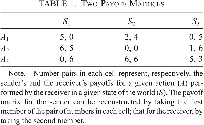
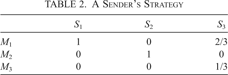
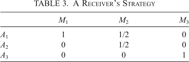
So, for example, a certain signaling game, SG, is univocally described by giving, first, the payoff matrices in table 1 and, second, the distribution for S (1/3, 1/3, 1/3)—that is, by stating that the three states the world can be in are equiprobable. And, for example, a sender-receiver configuration is individuated by SG together with the sender’s and receiver’s strategies in tables 2 and 3, respectively.

Table 1.

Two Payoff Matrices

	S 1	S 2	S 3
A 1	5, 0	2, 4	0, 5
A 2	6, 5	0, 0	1, 6
A 3	0, 6	6, 6	5, 3

Note. Number pairs in each cell represent, respectively, the sender’s and the receiver’s payoffs for a given action (A) performed by the receiver in a given state of the world (S). The payoff matrix for the sender can be reconstructed by taking the first member of the pair of numbers in each cell; that for the receiver, by taking the second member.

Table 2.

A Sender’s Strategy

	S 1	S 2	S 3
M 1	1	0	2/3
M 2	0	1	0
M 3	0	0	1/3

Table 3.

A Receiver’s Strategy

	M 1	M 2	M 3
A 1	1	1/2	0
A 2	0	1/2	0
A 3	0	0	1

That is, the sender will always send M ₁ in S ₁, and M ₂ in S ₂, and will throw a biased coin in S ₃, so as to send M ₁ with a probability of two-thirds and M ₃ with a probability of one-third. The receiver’s strategy can be read analogously.

In Lewis’s original discussion, the sender and receiver are rational agents with complex intentional profiles, and emphasis is put on sender-receiver configurations that achieve various kinds of equilibrium states. In Skyrms’s (Reference Skyrms1996, Reference Skyrms2010) groundbreaking reinterpretation of the Lewisian framework, in contrast, what counts is not the players’s rational appreciation of the payoff situation but the way in which various selection processes (evolution, reinforcement learning, and imitation) can shape the strategy of agents, who may be individually very unintelligent, as a result of those strategies being more or less successful in securing payoffs.

In the present article, we apply these methods to some long-standing questions about the relationship between communication and common interest. Many theorists, both in philosophy and other fields, have seen communication as a fundamentally cooperative affair, an interaction between agents whose interests are at least fairly well aligned. This has been a common theme across a range of literatures, including speech act theory (Grice Reference Grice1957), Millikan’s naturalistic theory of intentionality (Reference Millikan1984), and a range of recent work on the evolution of human behavior (Tomasello Reference Tomasello2008; Sterelny Reference Sterelny2012). Lewis himself assumed that common interest “predominates” in his original model (Reference Lewis1969/2002, 10). In the context of the Lewis model, there is common interest if sender and receiver tend to want the same acts performed in a given state of the world. Interests are divergent when the two agents want different pairings of actions and states. An intuition that many have shared is that if the interests of sender and receiver are too divergent, then a receiver will be unwise to trust anything a sender says. If receivers stop listening, there is no point in talking. So divergence of interests should eventually make communication collapse. This intuition is fundamentally a dynamic one; it predicts that when sender and receiver diverge enough in interests, a particular outcome should occur. How, then, do these ideas fare when cast in a formal model of behavioral change, using a dynamic version of the Lewis model? What role does common interest have in producing and maintaining communicative interactions? Those are the themes of this article.

Earlier work has already shed some light on this question. Skyrms (Reference Skyrms2010) considered a few cases of imperfect alignment of interests in a Lewis signaling model and showed that communication could be an equilibrium state in these cases. Skyrms discussed just a handful of cases, though. In their classic model from economics, Crawford and Sobel (Reference Crawford and Sobel1982) give a more general and rigorous treatment of the consequences of divergent interests for a static model that has both similarities and differences from the Lewis setup. They imagined a situation in which the sender wants to exaggerate her quality (or another relevantly similar state of the world), to some degree, and the receiver wants not to be taken in by the exaggeration. Crawford and Sobel found that as interests diverge more and more, fewer distinct signals can be used at equilibrium, until signaling collapses into a “pooling” outcome in which the sender makes no distinction between different states of the world. This result is in accordance with the intuition, outlined above, that when interests diverge too far, senders will say nothing worth listening to.

In both economics and biology, a rich set of models has been developed that explore the consequences of differential signal cost in enforcing honesty when interests diverge. When signaling itself is a costly action, there are situations in which it is plausible that only honest senders can afford to send a signal of a given kind. The first model to explore this idea was offered in economics by Spence (Reference Spence1973) and applied to the case of job markets. Zahavi, independently, soon after applied the same principle to biology (Reference Zahavi1975), where the choice of mates by females replaced the choice of employees (see also Grafen Reference Grafen1990a, Reference Grafen1990b; Maynard-Smith and Harper Reference Maynard-Smith and Harper2003; Zollman et al. Reference Zollman, Bergstrom and Huttegger2013). Since then, a wide range of models of this kind have been developed. In some models, the costs need only be operative when the population is not at equilibrium (Lachmann, Szamado, and Bergstrom Reference Lachmann, Szamado and Bergstrom2001).

The detailed development of costly signaling models may have fostered the impression that communication is very difficult to maintain in situations in which signal costs are entirely absent and interests do not align. Some well-known games do give this impression. However, this impression is somewhat misleading. In earlier work of our own (Godfrey-Smith and Martínez Reference Godfrey-Smith and Martínez2013), we used computerized search methods to assess the value of some exact measures of common interest as predictors of the viability of communication in a cheap talk Lewis model. By looking far outside the set of familiar games, we found that communication could persist in some situations characterized by extremely low levels of common interest. We also found a general predictive relationship between our measures of common interest and the viability of communication. This earlier work, however, focused entirely on the existence of Nash equilibria and contained no dynamical models.Footnote ¹ It did not investigate how accessible to evolution equilibria were.Footnote ² The current article considers the relationship between communication and common interest using dynamic methods. We ask how different degrees of common interest affect the evolutionary trajectories of populations of senders and receivers interacting in accordance with a Lewis model.

Section 2 describes the model used: a family of Lewis sender-receiver games, embedded in an evolutionary model on which quantitative measures of communication and common interest are defined. Section 3 discusses the main results regarding the relation between the degree of common interest present in a game and the maintenance of communication, while section 4 takes a closer look at the case of very low common interest. Section 5 assesses the significance of our results and offers conclusions.

2. The Model

Our model uses a Lewis sender-receiver game of the kind characterized in the introduction and then embeds this game in an evolutionary model in which change is described with the replicator dynamics (Hofbauer and Sigmund Reference Hofbauer and Sigmund1998, chap. 7; Sandholm Reference Sandholm2010, 126). Specifically, consider a signaling game, a set of possible sender’s pure strategies $S=\left\{{\sigma }_1,\dots ,{\sigma }_q\right\}$, and a set of possible receiver’s pure strategies $\Re =\left\{{\rho }_1,\dots ,{\rho }_r\right\}$. Instead of a single sender and a single receiver, we have a population of senders and another of receivers. The sender population can be characterized in terms of q behavioral types, each one of them implementing a different strategy in $S$, and their associated frequencies. The receiver population is, similarly, characterized by r types and their associated frequencies. The frequencies of the different sender and receiver types are $X=\left\{x_1,\dots ,x_q\right\}$ and $Y=\left\{y_1,\dots ,y_r\right\}$.

Members of the sender population are assumed to interact with members of the receiver population. The average payoff for the sender type that follows strategy ${\sigma }_i$ when dealing with a receiver following strategy ${\rho }_j$ is ${\pi }_{ij}^{\sigma }$. The receiver in that encounter gains ${\pi }_{ji}^{\rho }$. These payoffs are easily calculated from the payoff matrices, the players’ strategies, and the unconditional probabilities of states.

The average payoff for a sender type is the weighted average of the payoffs this type gets with each type present in the receiver population: ${\overline{\pi }}_i^{\sigma }=\sum _j{\pi }_{ij}^{\sigma }{y}_j$. Mutatis mutandis for the receiver: ${\overline{\pi }}_i^{\rho }=\sum _j{\pi }_{ij}^{\rho }{x}_j$.

Finally, the average payoff for the entire sender population is the weighted average of the averages per type: ${\overline{\pi }}^{\sigma }=\sum _i{x}_i{\overline{\pi }}_i^{\sigma }$. Mutatis mutandis for the receiver: ${\overline{\pi }}^{\rho }=\sum _i{y}_i{\overline{\pi }}_i^{\rho }$.

If sender and receiver populations follow the two-population replicator dynamics, the rate of change over time of the frequency of each type is given by the following differential equations:

(1)$\begin{array}{}{\dot{x}}_i=x_i\times \left({\overline{\pi }}_i^{\sigma }-{\overline{\pi }}^{\sigma }\right).\end{array}$

(2)$\begin{array}{}{\dot{y}}_i=y_i\times \left({\overline{\pi }}_i^{\rho }-{\overline{\pi }}^{\rho }\right).\end{array}$

We have now embedded a Lewis model within an evolutionary framework. Our next topic is the characterization of common interest between sender and receiver.

As in Godfrey-Smith and Martínez (Reference Godfrey-Smith and Martínez2013), we use C as a measure of common interest between sender and receiver. Parameter C formalizes the following idea: sender and receiver see perfectly eye to eye insofar as the outcome they most prefer coincides in every state, their second preference coincides too, and so on down to the least preferred outcome. Their interests diverge gradually as these preference rankings diverge.

Parameter C is calculated as follows. For each state (i.e., each column in the sender and receiver payoff matrices), we calculate the Kendall tau distance (the number of pairwise disagreements in the ranking of acts) between sender and receiver payoffs. For example, in the payoff matrix in table 1, the Kendall tau distance for state S ₁, ${\tau }_{S_1}$, is 2: sender and receiver disagree about which member is preferable in the pairs of acts (A ₁, A ₃) and (A ₂, A ₃) but agree that A ₂ is preferable to A ₁. Distance ${\tau }_{S_2}$ is 0: they agree completely on the preference ranking for acts in that state. Distance ${\tau }_{S_3}$ is also 2. An average distance is then calculated, using the unconditional probabilities of states as weights:

$\tau =\sum _i\text{Pr}\left(S_i\right){\tau }_{S_i}.$

Finally, τ is rescaled so as to have 0 as no common interest and 1 as perfect common interest. For n states this yields

$C=1-\frac{2\tau }{n(n-1)}.$

Parameter C is a very coarse-grained measure of common interest.Footnote ³ In games with three equiprobable states and three acts, there are only 10 possible values of C. However, as we will see, it is strongly predictive of the possibility of communication.

Next we consider how to describe communication itself in such a setup. We say that a sender-receiver configuration contains informative signaling when the signals sent carry some information about the state of the world, and the acts performed carry information about the signal sent. These relationships are measured as mutual information. This is a widely used concept, originally due to Shannon (see Shannon and Weaver Reference Shannon and Weaver1949), that measures the amount of association between two variables, the extent to which the value of one predicts the value of the other. Mutual information is symmetrical, and its value ranges between a minimum of 0 (no association) and a maximum dependent on the amount of entropy (uncertainty) in the two variables. It is calculated as follows.

The (unconditional) entropy of states is given by

$H\left(S\right)=-{\sum }_i\text{Pr}\left(S_i\right){\text{log}}_2\left(\text{Pr}\right(S_i\left)\right).$

And the entropy of states conditional on acts is given by

$H\left(S\right|A)={\sum }_i\text{Pr}(A_i\left)H\right(S|A=A_i),$

where $\text{Pr}\left(S_i\right)$ is the unconditional probability of state S_i. Finally, the mutual information between states and acts is given by

$I(S;A)=H\left(S\right)-H\left(S\right|A).$

In games with three states, three messages, and three acts, if $I(S;A)={\text{log}}_{2}3$, the sender’s strategy is a bijection between S and M, and the receiver’s strategy a bijection between M and A. We will refer to configurations in which both sender’s and receiver’s strategies have this property as signaling systems—we take this notion from Lewis (Reference Lewis1969/2002), but our use differs from his in that we are placing no constraints on the payoffs received by sender and receiver, while for Lewis players engaging in a signaling system always obtain maximum payoffs. If I(S; A) = 0, nothing whatsoever can be said about the state of the world from the act the receiver performs—this corresponds to the absence of communication.

Next we describe the relationships between the states of populations of senders and receivers, on one hand, and the measure of communication outlined above. As we have set up our model, at any given time a range of different types may exist in each of the two populations—the sender population and receiver population. Thus, a great range of different communicative interactions is assumed to be taking place—there is not a single sender-receiver configuration present, in the sense we introduced earlier. However, we aim to give a general characterization of the sender-receiver relationships that exist at each time. We do this in a way that has become common in models of this kind; we “translate” the pair of population structures that are present at a time into a single sender-receiver configuration by averaging over the different individual-to-individual interactions that are possible given the state of the two populations.Footnote ⁴ For each state of the world, there is a probability distribution over messages that is determined by the state of the sender population. Thus, there is a population-wide “sender’s strategy” instantiated for that state. Similarly, for each available message, there is a probability distribution over acts that is determined by the state of the receiver population, and hence a population-wide “receiver’s strategy” instantiated for that message. The combination of these population-wide strategies plus the unconditional probability of states determines the mutual information between states and acts.

3. Results

Our main research question was how the presence of communication relates to common interest. We look into this question by generating a large number of random signaling games at each level of common interest and then recording how likely it is in these games that random starting points evolve to a situation in which communication happens, depending on the level of common interest. Specifically, we focus on cheap talk signaling games with three equiprobable states, three messages, and three acts. There are 10 possible values of C, our measure of common interest, for games of this sort. These games are individuated by 18 numbers: the 18 values in a payoff matrix of the form seen in table 1.

For each value of C, we generated 1,500 collections of 18 random integers between 0 and 99. Each one of these collections individuates a signaling game. A population of senders (the same applies to receivers) is characterized in terms of the frequencies of the 27 types of pure strategists who may be present. These pure strategies can be represented as follows, using the convention introduced in tables 2 and 3 in the introduction:

$\left(\begin{array}{ccc}1& 1& 1\\ 0& 0& 0\\ 0& 0& 0\end{array}\right),\left(\begin{array}{ccc}1& 1& 0\\ 0& 0& 1\\ 0& 0& 0\end{array}\right),\dots ,\left(\begin{array}{ccc}0& 0& 0\\ 0& 0& 0\\ 1& 1& 1\end{array}\right).$

For each of the 1,500 random games per value of C, we ran simulations starting from 1,000 different randomly chosen states of the two populations (the sender and receiver populations). This is equivalent to choosing 1,000 random ordered pairs of points in the 26-dimensional simplex. At t = 1,000, the pair of resulting population states was “translated” into a sender-receiver configuration, in the way described above, and the mutual information between states and acts was recorded. When the sender-receiver configuration at t = 1,000 showed nonzero mutual information between states and acts, we scored that simulation as one in which communication evolves. In total, then, 10 (values of C) times 1,500 (random games) times 1,000 (pairs of random starting frequencies) simulations were run (1.5 × 10⁷ simulations).

We next note some implementation details. First, no effort was made to check whether by t = 1,000 populations had settled into any specific kind of equilibrium or cyclic behavior, although casual inspection shows this to be often the case. Similarly, we have not checked for the stability, in any formal sense, of t = 1,000 states; we have not assessed the consequences of small hypothetical deviations from these states.

Finally, to prevent rounding errors from affecting the results, we only count as nonzero amounts of information above 10⁻³ bits. It is possible, if unlikely, that rounding errors still play a role in the final results: calculations are carried out using 64-bit floating-point numbers. In the computer we used, this means that the minimum frequency for a population is around 2 × 10⁻³⁰⁸, types that go below this frequency simply becoming extinct. In the replicator dynamics it is impossible for a frequency to decline to exactly zero, so it is in principle possible that this computational limitation introduces a distortion: that is, it is in principle possible that types below the 2 × 10⁻³⁰⁸ mark would have bounced back to nonnegligible frequencies. But this number is so low that the empirical relevance of results that depended on types bouncing back from such a frequency would be doubtful.

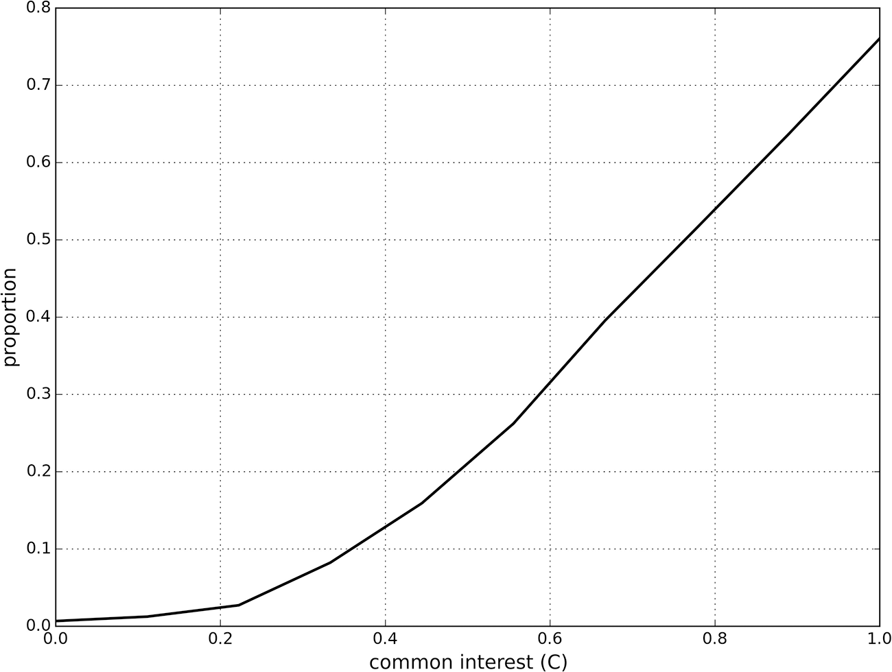
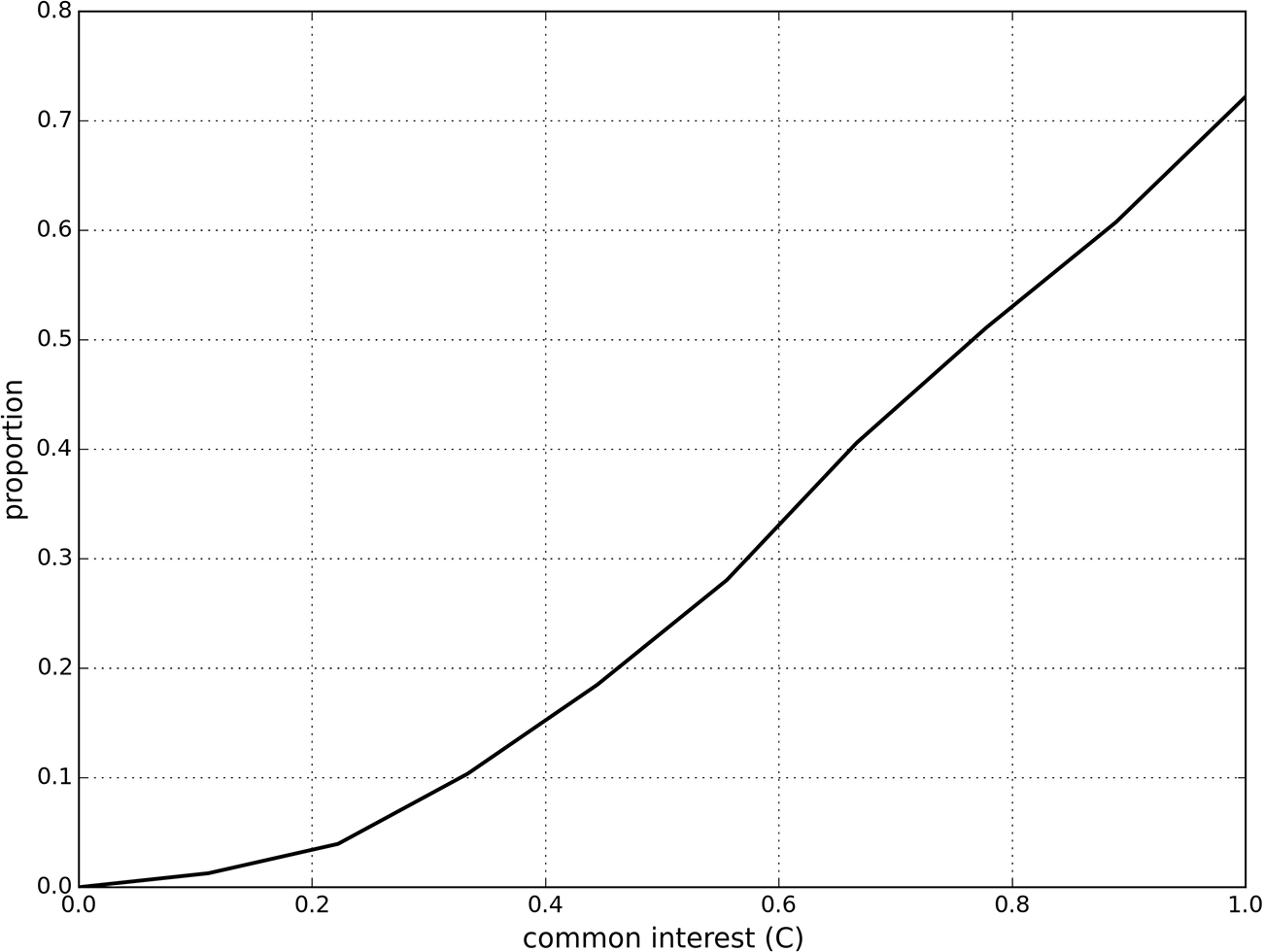
A coarse-grained summary of the results of these simulations is given in figure 1. This figure shows, for each value of C, the overall proportion of simulations in which communication evolved. So we here group together, within each value of C, all the games with that value of C and all the initial states for each game. We then find, as shown in figure 1, that C is very predictive of this proportion: there are very few cases of the evolution of communication when C = 0 (although there are some; see sec. 4 for discussion), while this is by far the most likely outcome when C = 1.Footnote ⁵ The dependence of communication evolution on C is monotonic and appears to be smooth across the chart (although bear in mind that there are only 10 values of C, and curve fitting is therefore not entirely meaningful).

Figure 1.

Proportion of simulations in which communication evolves, expressed as a function of common interest.

In previous work, as noted in the introduction, we carried out an analysis of the prevalence of communicative Nash equilibria in samples of games with different values of C. This work used the same criterion for an “information-using” outcome that we employ here, although in the earlier article this criterion only characterized equilibrium states. Our dynamic analysis in this article confirms the conclusions drawn about the predictive value of C in the earlier work. In particular, the proportion of outcomes in which communication evolves, for each value of C, in the dynamic analysis is strongly correlated with the proportion of games, for each value of C, that contain an information-using Nash equilibrium as found in the earlier study. The Pearson correlation coefficient between the two series of values is .9990 (with p < .001). Thus, the results of the dynamic model of this article do appear to validate the findings of the earlier static analysis of the role of C in maintaining communication.

4. Communication at Very Low Values of C

As figure 1 shows, in some games with C = 0 we find a few starting points that evolve to situations in which communication is sustained by t = 1,000. A value of C = 0 only obtains when the preferences of sender and receiver are reversed everywhere. That is, the most preferred act for the sender is the act least preferred by the receiver, and conversely, in every state. Remarkably, even in such a situation some simulations (10,000 out of half a million runs, in our sample) can accommodate communication. But this feature of our results does show some sensitivity to the dynamics chosen: when we ran the same simulations using the replicator-mutator dynamics, there were no runs in which a C = 0 game evolved to maintain communication at t = 1,000. (Details of this analysis are given in the appendix.)

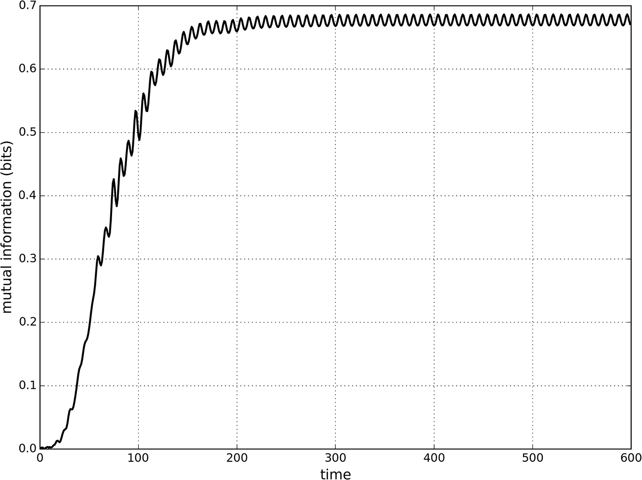
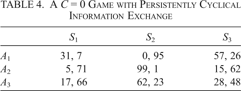
A further notable feature of the dynamic results is that no simulation in our C = 0 sample evolved toward a Nash equilibrium in which information was being exchanged (although in some C = 0 games an information-using Nash equilibrium does exist.) This is evident from the fact that no such simulation was approaching an information-exchanging state (Nash or not) in which frequencies of behaviors had ceased to change by t = 1,000. Instead, most of the C = 0 configurations at t = 1,000 in which informative signaling is taking place belong to persisting cycles.Footnote ⁶ As an example, figure 2 shows the evolution of mutual information corresponding to a simulation based on the game in table 4: very quickly, in a couple hundred generations, the mutual information between states and acts enters a persisting cycle between 0.67 and 0.69 bits.

Figure 2.

A C = 0 game evolving to cyclic communicative behavior.

Table 4.

A C = 0 Game with Persistently Cyclical Information Exchange

	S 1	S 2	S 3
A 1	31, 7	0, 95	57, 26
A 2	5, 71	99, 1	15, 62
A 3	17, 66	62, 23	28, 48

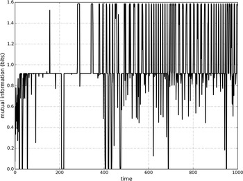
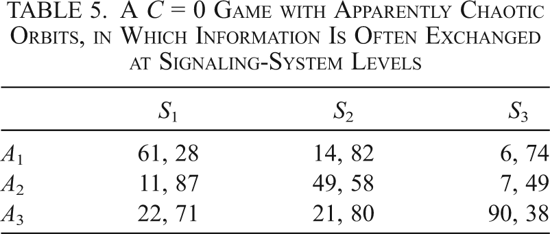
Some other C = 0 games did not give rise to cycles by t = 1,000 but instead appeared to generate a chaotic dynamical regime. Results of this kind have also been found in a dynamic model of a Lewis signaling game by Wagner (Reference Wagner2012). Wagner used a stronger criterion for complete conflict of interest than C = 0 (he understood complete conflict of interest to exist only in constant sum games). Some of our simulations (such as the one corresponding to fig. 3 and table 5) often show communication at signaling-system levels. That is, the very incompatible preference rankings of sender and receiver can still sustain simulations in which the sender is, roughly half of the time, perfectly informative about the state of the world, and the receiver perfectly mindful of this information.Footnote ⁷

Figure 3.

One evolution of mutual information between states and acts for the game presented in table 5.

Table 5.

A C = 0 Game with Apparently Chaotic Orbits, in Which Information Is Often Exchanged at Signaling-System Levels

	S 1	S 2	S 3
A 1	61, 28	14, 82	6, 74
A 2	11, 87	49, 58	7, 49
A 3	22, 71	21, 80	90, 38

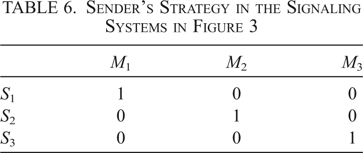
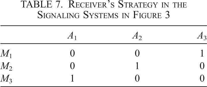
The signaling system that keeps recurring in the simulation corresponding to figure 3 is described in tables 6 and 7: the sender is perfectly informative, and the receiver exploits this to her benefit and the sender’s detriment—although the receiver does not carry the exploitation to the fullest extent; see below.

Table 6.

Sender’s Strategy in the Signaling Systems in Figure 3

	M 1	M 2	M 3
S 1	1	0	0
S 2	0	1	0
S 3	0	0	1

Table 7.

Receiver’s Strategy in the Signaling Systems in Figure 3

	A 1	A 2	A 3
M 1	0	0	1
M 2	0	1	0
M 3	1	0	0

What is sustaining informative signaling at C = 0 in these two kinds of cases (periodic orbits on the one hand, apparently chaotic orbits on the other)? There appears to be a main pattern in all of them: given that sender’s and receiver’s preferences are exactly reversed, the receiver would generally like to exploit any information in the messages sent by the sender—that is, use it to act in a way beneficial to her but detrimental to the sender. But any exploitation by the receiver will have to involve letting her behavior be guided by the messages sent by the sender. This means the sender can exploit her attempted exploitation, by remapping states to signals in a way beneficial to her but detrimental to the receiver.

Godfrey-Smith (Reference Godfrey-Smith and Stegmann2013) describes one very simple kind of evolution that obeys this pattern: in a C = 0 game, if a sequential best-response regime is in place (the sender’s strategy at t is the best response to the receiver’s strategy at t − 1, which, in turn, is the best response to the sender’s strategy at t − 2, etc.) and the sender kicks off the process by sending fully informative signaling (i.e., by using a strategy that is a bijection between S and M), then at any given time, the sender is mapping states to messages one-to-one, and the receiver mapping messages to acts one-to-one. Every configuration is a signaling system, but not as a result of good will: they are taking turns to exploit each other.

The persisting cycles in our C = 0 sample also appear to conform to this sequential exploitation pattern. Consider again the game in table 4. Figure 4 is a fine-grained representation of the evolution of sender and receiver frequencies for the particular simulation that generated the results shown in figure 2; figure 2 shows change in mutual information while figure 4 shows change in the frequencies of the underlying behaviors.

Figure 4.

Evolution of frequencies in a persisting cycle for the game in table 4.

In what follows, we use S[M N O] as an abbreviation of the pure sender strategy consisting in sending (only) message M in S ₁, message N in S ₂, and message O in S ₃. And R[P Q T] stands for the pure receiver strategy that consists of doing (only) act P in response to M ₁, act Q in response to M ₂, and act T in response to M ₃.

In the cycle, represented in figure 4, the only two types with nonzero frequencies in the receiver population are R[1 3 3] and R[2 3 3]. That is, the receiver always responds to M ₂ and M ₃ with A ₃ and mixes A ₁ and A ₂ in response to M ₁. The sender strategies with highest frequency are S[2 1 1] and S[2 2 1]. That is, the population mostly contains strategies that always send M ₂ in S ₁ and M ₁ in S ₃, but the strategies differ in how they respond to S ₂, with the result that there is a population-wide mixing of M ₁ and M ₂ in response to that state. There is a small proportion of senders (below 10%) doing S[2 3 1] and S[3 1 1].

The frequencies of types R[1 3 3] and R[2 3 3] in the receiver’s population change at the same rate as the proportions of S[2 1 1] and S[2 2 1] in the sender’s population, only with a lag of approximately 3 time units. Here is what is going on: when the proportion of M ₁ sent by the sender in S ₂ falls, M ₁ becomes more informative about S ₃. In that case, the receiver wants to respond to M ₁ with A ₂, which secures the highest payoff for the receiver in S ₃ (and is exploitative, insofar as the sender is then stuck with the lowest payoff in S ₃). Consequently, the frequency of the R[2 3 3] type increases in the receiver population. As this frequency increases, the strategy consisting of sending M ₁ in S ₂ becomes more attractive for the sender (the pair S ₂/A ₂ has a very high payoff for her), and thus S[2 1 1] increases its frequency. Which again brings the frequency of R[1 3 3] up, and so on.

Sender and receiver populations are thus launched in a cycle of sequential exploitation, but this is not all that is going on. For example, M ₁ is, throughout, never sent in S ₁. This gives a substrate of more cooperative and stable communication to the regime of attempted mutual exploitation: throughout the process, the receiver, when confronted with M ₁, can rest assured that S ₁ is not the case. Apparently, then, these cases should be understood in terms of a pair of phenomena, one cooperative and one noncooperative. We outlined the role of exploitation above; here we will briefly attempt to characterize the second phenomenon, which involves a subtle form of cooperation. Sender and receiver can be seen as transforming, by means of mixed strategies, one game into another. Suppose that a sender sends M ₁ always in S ₁, mixes M ₁ and M ₂ in S ₂, and never sends M ₁ in S ₃. Then when the sender sends M ₁, she confronts the receiver with an “uncertainty bundle” that is partly composed of S ₁ and partly composed of S ₂.Footnote ⁸ The sender can be seen as giving the receiver perfect information about a bundle, rather than imperfect information about the “raw” state. A receiver, too, can create a bundle. When the receiver mixes A ₁ and A ₂, for example, in response to a given message, the sender is presented with a bundle of acts that the sender must treat as a unit when determining when to send that message.

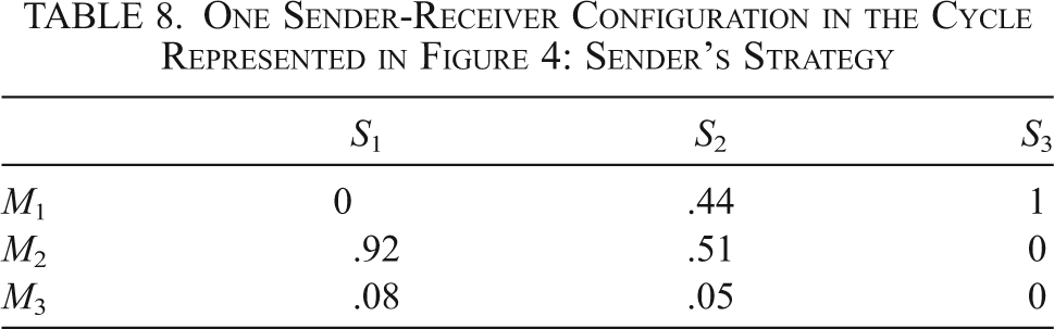
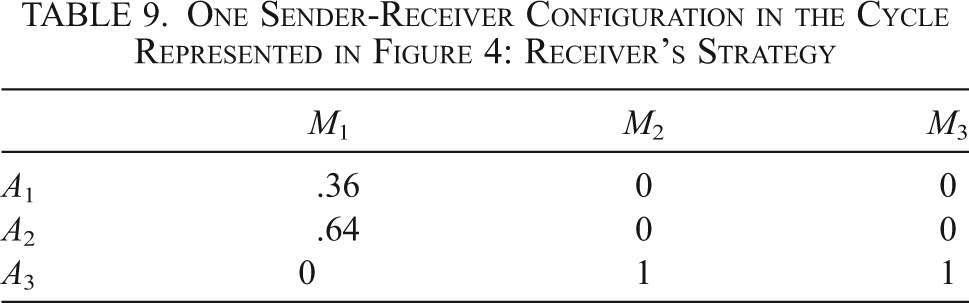
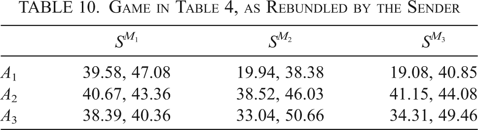
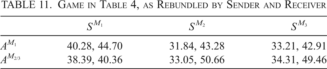
Suppose, then, we revisit the game in table 4 and consider the situation that obtains when the sender and receiver are following, for example, the strategies given in tables 8 and 9, which happen halfway through figure 4. We can redescribe this situation as one in which the senders are being perfectly informative about three “uncertainty bundles” they have constructed. The new “game” is shown in table 10, where S^M_i stands for the bundle of states that the sender is presenting with message M_i. Here, sender and receiver agree on the worst act (the worst “raw” act, not the worst bundle of acts) possible in each state, and the new value of C is 0.66. Further, though, we can treat the receivers as creating bundles of acts: they are offering a new “act,” A^M₁, which roughly consists of one-third of A ₁ and two-thirds of A ₂, and withdrawing access to the pure A ₁ or A ₂. If we reinterpret the game as transformed by both the sender’s and receiver’s bundling, we reach the payoff matrices shown in table 11. This is now a “game” with complete common interest: both sender and receiver prefer A^M₁ in S^M₁, and A ^{M _2/3} (the old A ₃) in the other two state bundles. Because this “game” can be transformed again by either player changing his or her behaviors, and hence their bundling, the existence of common interest here does not have the same role that it has in an underlying game that acts as a fixed constraint. But we think that this description in terms of bundling may yield some understanding of how communication can arise in these apparently unlikely contexts.

Table 8.

One Sender-Receiver Configuration in the Cycle Represented in Figure 4: Sender’s Strategy

	S 1	S 2	S 3
M 1	0	.44	1
M 2	.92	.51	0
M 3	.08	.05	0

Table 9.

One Sender-Receiver Configuration in the Cycle Represented in Figure 4: Receiver’s Strategy

	M 1	M 2	M 3
A 1	.36	0	0
A 2	.64	0	0
A 3	0	1	1

Table 10.

Game in Table 4, as Rebundled by the Sender

	S M 1	S M 2	S M 3
A 1	39.58, 47.08	19.94, 38.38	19.08, 40.85
A 2	40.67, 43.36	38.52, 46.03	41.15, 44.08
A 3	38.39, 40.36	33.04, 50.66	34.31, 49.46

Table 11.

Game in Table 4, as Rebundled by Sender and Receiver

	S M 1	S M 2	S M 3
A M 1	40.28, 44.70	31.84, 43.28	33.21, 42.91
A M 2/3	38.39, 40.36	33.05, 50.66	34.31, 49.46

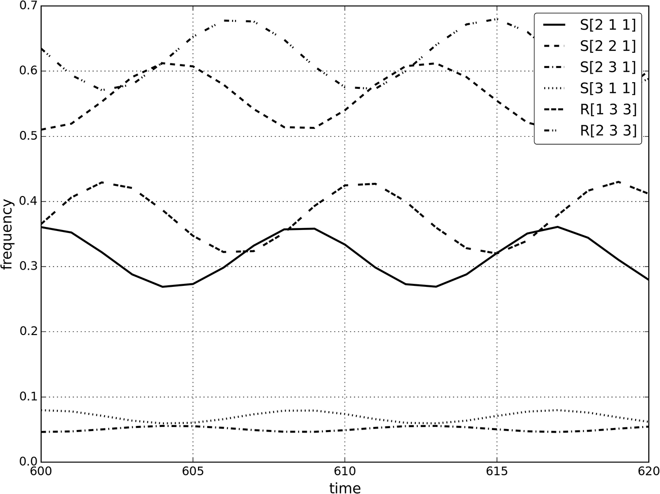
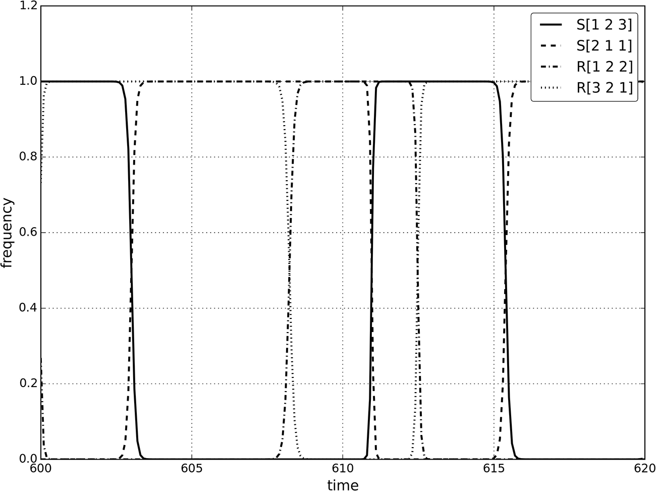
It is more difficult to provide an intuitive description of what it is that forces senders and receivers into their behavior in the chaotic regimes that sometimes emerge in the game presented in table 5. A common pattern in the emergence of signaling systems in these regimes is quasi-periodic behavior in both sender and receiver, with two similar, but off-sync, “periods.” For example, from t = 600 to t = 620 in the simulation corresponding to figure 3, the sender alternates S[2 1 1] with S[1 2 3]. Meanwhile, the receiver alternates R[3 2 1] with R[1 2 2]. As the sender’s “cycle” is out of sync with the receiver’s, all four combinations occur: S[2 1 1] and R[3 2 1], S[1 2 3] and R[3 2 1], S[2 1 1] and R[1 2 2], S[3 2 1] and R[1 2 2]. The second among these combinations is a signaling system. The other three are partially informative, thus the 1.58 bits/0.91 bits alternation in figure 3 between t = 600 and t = 620.

In fact, by the time senders and receivers engage in this behavior, the frequencies of most sender and receiver types is zero; in particular, the reason why the receiver does not respond to S[1 2 3] with R[2 1 1] is that this type is extinct by t = 600. The best the receiver can do is engage in signaling-system behavior, with R[3 2 1]. What we see is sequential exploitation to the full extent of their current capabilities. In the case we have been discussing, the difference between frequencies that are very close to zero and those that are effectively zero (below 2 × 10⁻³⁰⁸; see above) turns out to be very important: as figure 5 shows, frequencies jump from extremely close to zero to extremely close to one, and, if we round population frequencies so that every type with frequency below 10⁻¹⁰ is declared extinct, signaling systems fail to appear.

Figure 5.

Detail of the evolution of populations corresponding to figure 3, between t = 600 and t = 620.

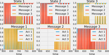
The above analysis, in any case, only focuses on one particularly legible fragment of the simulation. Most of what happens in the full run depends on haphazard details of the population structure, as is bound to happen in apparently chaotic behavior of this sort, and could not be convincingly labeled as sequential exploitation. The unpredictable alternation of quasi-periodic patterns that can be noticed in a longer run is shown in figure 6, which presents the evolution of the sender-receiver configurations to which the population structure translates between t = 600 and t = 800.

Figure 6.

Evolution of sender-receiver configurations corresponding to figure 3, between t = 600 and t = 800.

As we have said, none of the C = 0 runs in our sample in which communication is maintained evolve toward a Nash equilibrium. In fact, in our sample, the first case in which there is evolution toward a Nash equilibrium happens at C = 0.22. Somewhat surprisingly, the situation appears to be at follows. On one side, we have anecdotal evidence to the effect that when a C = 0 game does have a Nash equilibrium in which communication is maintained, then it is very likely that some initial population frequencies will lead to persisting communication: in all of the 24 such games we have found in the random sampling prepared for this and our previous article, the replicator dynamics will take some initial conditions to a state at t = 1,000 in which communication does then persist. On the other side, in no case that we have found is there evolution toward the Nash equilibrium itself.

5. Conclusion

This article describes the results of a dynamic analysis of the role of common interest in the evolution of communication in a three-state Lewis signaling game. We find a strong predictive role for common interest, as measured by C: in a large random sample of games, the proportion of evolutionary simulations in which communication was maintained at t = 1,000 was monotonically associated with C. The results presented here complement those in an earlier article (Godfrey-Smith and Martínez Reference Godfrey-Smith and Martínez2013) that gave a purely static analysis of games of this kind, also using C as a measure of common interest. The two sets of results are broadly consistent and complementary; each approach provides a different perspective on these systems.

First, an analysis using Nash equilibria can be used to give a coarse-grained description of a range of systems that operate under different dynamical regimes and also cases involving human choice in which no well-defined “dynamic” may exist at all. The replicator-dynamic model, however, gives a much finer-grained representation of systems to which it applies and has been shown to be informative about systems that follow a somewhat different dynamic, as well (Bendor and Swistak Reference Bendor and Swistak1998).

Our work here also uncovers phenomena that involve cycling and apparently chaotic behaviors. We offered an initial analysis of these outcomes in terms of a combination of sequential exploitation and the transformation of games through “uncertainty bundling,” but this last analysis was offered briefly, as a first foray; clearly much more work remains to be done on the interaction between common interest and evolutionary dynamics in signaling games.