


1. INTRODUCTION
When you find yourself disagreeing with an epistemic peer, how (if at all) should you revise your credence in the disputed proposition? This question has generated an extensive literature over the past decade. Following custom, we can broadly divide different views of disagreement into a “steadfast” camp and a “conciliatory” camp. Roughly, according to steadfast views, one is typically permitted to stick to one's guns and maintain one's credence in the face of peer disagreement. By contrast, conciliatory views maintain that one is typically required to revise one's credence in the direction of one's peer.Footnote 1
For all their differences, there is a broad consensus among contenders in the disagreement debate that evidence of disagreement is a kind of higher-order evidence – roughly, evidence about the existence or bearing of ordinary first-order evidence.Footnote 2 There is, however, little consensus about how to understand the normative impact of higher-order evidence. On the one hand, David Christensen has argued that higher-order evidence can require an agent to “put aside” or “bracket” her ordinary first-order evidence, thereby preventing the agent from giving the original first-order evidence its due (Christensen Reference Christensen2010: 195). In particular, on Christensen's view, the higher-order evidence in cases of peer disagreement serves to cancel or undermine the normative impact of the first-order evidence. This, in turn, naturally aligns with the conciliatory dictum that parties to a peer disagreement should revise their opinions in a uniform way, regardless of who judged the first-order evidence correctly to begin with. On the other hand, Thomas Kelly has argued that the higher-order evidence in cases of peer disagreement does not generally “swamp” or undermine the normative impact of the first-order evidence (Kelly Reference Kelly, Goldman and Whitcomb2010: 192). This view, in turn, aligns with the steadfast dictum that disagreeing peers should revise their opinions in a way that properly reflects who judged the original first-order evidence correctly to begin with. As such, the divide between steadfast and conciliatory views of disagreement seems to stem, at least partly, from a more general divide over how to understand the epistemic significance of higher-order evidence. It is therefore natural to expect that general considerations about higher-order evidence may help us to better understand and adjudicate between different views of the epistemic significance of disagreement.
In this paper, we outline (§2) a simple formal framework for determining the epistemic significance of a body of higher-order evidence, and use this framework (§3) to motivate a novel interpretation of the popular “equal weight view” of disagreement – we call it the Variably Equal Weight View (VEW). According to VEW, disagreeing peers should always be given equal weight, but the amount of weight they should be accorded varies depending on how reliable they are: roughly, reliable peers should be given equal high weight, and unreliable peers should be given equal low weight. We show (§4) that VEW differs from the standard Split the Difference (SD) interpretation of the equal weight view in almost all cases of disagreement, and use our formal framework to explain why SD has seemed attractive but is in fact misguided. A desirable feature of VEW, we argue (§5), is that it gives rise to plausible instances of what Easwaran et al. (Reference Easwaran, Fenton-Glynn, Hitchcock and Velasco2016) call synergy – an effect whereby the parties to a disagreement should become more (or less) confident in the disputed proposition than any of them were prior to the disagreement. Lastly, we generalize VEW to cases of non-peer disagreement (§6).
2. HIGHER-ORDER EVIDENCE
Let us begin by characterizing higher-order evidence more precisely. As of yet, there is no single, generally agreed upon definition of higher-order evidence in the literature, but higher-order evidence has been variously characterized as “evidence of my own rational failure” (Christensen Reference Christensen2010: 185), “[e]vidence about the existence, merits, or significance of a body of evidence” (Feldman Reference Feldman2009: 304), or “evidence that suggests that the bearing of the original, first order evidence is something other than what one initially took it to be” (Kelly Reference Kelly, Goldman and Whitcomb2010: 200).Footnote 3 To illustrate, consider a paradigmatic higher-order case adapted from Christensen (Reference Christensen2010: 187):
Performance-diminishing drug: Suppose I carefully prove a logical theorem T. Since I know myself to be a competent logician, I become confident that T is in fact a theorem. However, my doctor now calls to tell me that she has given me a performance-diminishing drug that subtly but significantly impairs my reasoning abilities. In light of this new information, I become less confident that my proof is sound and that T is in fact a theorem.
Here, the doctor's testimony seems to rationalize a change of belief in T, not by speaking directly for or against T, but by indicating that my reasons for being confident in T are weaker than I initially took them to be. So the doctor's testimony is higher-order evidence against T. Conversely, if we had replaced the performance-diminishing drug by a performance-enhancing drug, the doctor's testimony would have been higher-order evidence for T.
More generally, we will say that a body of evidence is first-order iff it bears on what we will call a first-order hypothesis: an ordinary proposition such as “the sun is shining” or “2 + 3 = 5.” Similarly, we will say that a body of evidence is higher-order iff it bears on what we will call a higher-order hypothesis: a proposition about an evidential relation between a first-order hypothesis and a body of first-order evidence. We can think of higher-order hypotheses as propositions of the form “this-or-that evidence bears on this-or-that hypothesis in this-or-that way.” For example, the hypothesis that “my calculations do not support that T is a theorem” is higher-order in virtue of being about an evidential relation between a body of first-order evidence (my calculations) and a first-order hypothesis (“T is a theorem”). Formally, we will represent higher-order hypotheses using a standard probability function P which, given a hypothesis and a body of evidence, yields a sharp probability of the hypothesis given the evidence. For example, we will write P(H|E) = .57 to say that the probability of hypothesis H given evidence E is .57.Footnote 4 We will assume that rational credences conform uniquely to P – that is, a rational agent with total evidence E bearing on H has a credence in H that is identical to P(H|E).Footnote 5 This assumption, together with the assumption that evidential probabilities are sharp, implies what Feldman (Reference Feldman and Antony2007) has labelled “the uniqueness thesis”: for any body of evidence bearing on some hypothesis, there is a unique credence that is rational to have in that hypothesis given that evidence. The equal weight view is often thought to be tightly connected to the uniqueness thesis. For instance, Feldman (Reference Feldman and Antony2007) argues that the uniqueness thesis commits one to the equal weight view, and Kelly (Reference Kelly, Goldman and Whitcomb2010) argues, conversely, that the equal weight view is implausible (partly) because it presupposes the uniqueness thesis. Yet, it remains contentious how (if at all) the equal weight view is connected to the uniqueness thesis, and we will not pursue this question here.Footnote 6
Another central distinction will be that between first-order and higher-order probabilities. If H is a first-order hypothesis and H H is a higher-order hypothesis, then P(H|ċ) is a first-order probability, and P(H H |ċ) is a higher-order probability. For example, we write P(P(H|ċ) = .57|ċ) = .3 to say that there is a higher-order probability of .3 that the first-order probability of H is .57. For ease of notation, we will henceforth use a higher-order probability function defined as
 $$Q(\,p) = _{df} P(P(H \vert \cdot ) = p \vert \cdot ),$$
where H is a given first-order hypothesis, and p is a probability variable. Given this, we can simply write Q(.57) = .3 to say that there is a higher-order probability of .3 that the first-order probability of H is .57. As usual, first-order and higher-order probabilities may or may not be conditional on evidence.
If we know the higher-order probability distribution Q(p) for a first-order hypothesis H, the Law of Total Probability (LoTP) offers a simple way of determining the first-order probability of H:
 $$P(H \vert \cdot ) = \sum\limits_{i = 1}^n p_i Q(\,p_i )\,\,\,\,{\rm (LoTP)}$$
This formulation of LoTP presupposes that p is a discrete probability variable that can take on n different values p 1, …, p n . If p is continuous, the finite sum above will instead be an integral over the unit interval [0,1], and Q(p) will be a density function. Here is a simple example of how to use LoTP:
Two kinds of dice: You are about to roll a random die from a bowl of dice, and you have conclusive evidence (E
H
) that half of the dice are three-sided, while the other half are six-sided. Before picking a die, you consider the likelihood that (H) you will roll a six. In light of your evidence, you are rationally certain that there is a .5 chance that the die is three-sided, and similarly a .5 chance that it is six-sided. And while there is no chance of rolling a six if the die is three-sided, there is a one-sixth chance of doing so if the die is six-sided. So
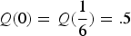 $Q(0) = Q(\displaystyle{1 \over 6}) =. 5$
. By plugging these higher-order probabilities into LoTP, we can calculate the first-order probability of H given E
H
as follows:
 $P(H\vert E_H ) = 0 \cdot. 5 + \displaystyle{1 \over 6} \cdot. 5 \approx 8\% $
.
The central benefit of this formal setup is that it allows us to capture how a body of higher-order evidence can make a difference to the evidential probability of a first-order hypothesis H, not by speaking directly for or against H, but by influencing the shape of the higher-order probability distribution for H. Obviously, the question remains what the higher-order probability distribution Q(p) will look like given different bodies of evidence, and, in particular, how we should determine Q(p) in cases where an agent possesses a mixed body of first-order and higher-order evidence. But if we can answer this question, LoTP can help us calculate the resulting first-order probability.
In the next section, we will use the core intuition behind the equal weight view to specify the higher-order probability distribution Q(p) in cases of peer disagreement. We choose to focus our attention on the equal weight view partly because of its prominence in the literature, and partly because it remains the best game in town to our mind. Yet, we are optimistic that our higher-order approach may be used to interpret other positions in the disagreement debate as well.
3. THE VARIABLY EQUAL WEIGHT VIEW
Consider a paradigmatic case of peer disagreement adapted from Levinstein (Reference Levinstein2015: 1):
Weather forecasters: Each morning, two equally experienced weather forecasters assess the same body of meteorological data and make private predictions of whether it will rain later that day. This morning, they learn that their predictions conflict: one has predicted that it is going to rain, while the other has predicted that it is not going to rain. How (if at all) should they revise their weather forecasts?
According to the equal weight view, in revising their weather forecasts, the disagreeing weather forecasters should place equal weight on each other's predictions. The driving intuition is that, absent reasons to think that I'm in a better epistemic position than you with respect to some proposition, it seems arbitrary and question-begging of me to place more weight on my own opinion just because it's mine.Footnote 7
Compelling as it is, the equal weight dictum, in its bare form, underdetermines how disagreeing peers should revise their opinions. For the mere requirement that disagreeing peers should place equal weight on each other's opinions leaves open just how much weight they should so place. For example, the weather forecasters from above can strictly speaking satisfy the equal weight dictum by placing no weight at each other's predictions whatsoever. Yet, this would seem to go against the spirit of the equal weight dictum. On a more plausible interpretation, the weather forecasters should place an amount of weight on each other's predictions that properly reflects how competent or reliable they are at judging the meteorological data: if they are reliable at judging the data, they should place equal high weight on each other's predictions, and if they are unreliable at judging the data, they should place equal low weight on each other's predictions.
In light of these considerations, we propose the following qualification of the equal weight dictum:
The variably equal weight dictum: Disagreeing peers should always place equal weight on each other's opinions, but the amount of weight they should accord each other depends on how reliable they are at judging the shared first-order evidence.
In the remainder of this section, we will use the formal tools introduced in
 ${\rm \S}$
2 to make the variably equal weight dictum precise. As a first step, we need a general characterization of peer disagreement cases that specifies how reliable the disagreeing peers are at judging the available evidence. To this end, we will use the following template:
Peer disagreement: Two agents a and b share their total body of first-order evidence E bearing on a first-order hypothesis H. The agents are rationally certain that they both have a reliability of r – that is, they are both certain that there is a probability of r that a will judge E correctly, and similarly for b. The agents form independent opinions about the bearing of E on H: a judges that P(H|E) = p a , and b judges that P(H|E) = p b . Which credence should the agents adopt in H upon disagreement?
Let us clarify a few points about the notion of reliability used here. We represent an agent's reliability by a real number r ∈ [0, 1] that denotes the probability, prior to judging a body of evidence, that the agent will judge the evidence correctly (i.e. make a judgment identical to the true evidential probability). For example, if an agent with a reliability of .3 judges that P(H|E) = .9, then there is a probability of .3 that, in fact, P(H|E) = .9, and, accordingly, a probability of .7 that P(H|E) ≠ .9.Footnote 8 This notion of reliability is intentionally idealized. Presumably, agents like you and I rarely (if ever) judge evidence in this highly precise way. Later, in §6, we introduce a more sophisticated model of reliability which is roughly designed to represent the probability that an agent's judgment is at least “in the right ballpark.” But for now, we stick to the idealized representation to keep the formalism simple.
Our notion of reliability is “evidence-based” in the sense that it captures an agent's ability to judge the evidence at hand. As such, it differs importantly from “truth-based” notions of reliability that capture how well an agent's credences track the truth. Truth-based notions of reliability are useful for a number of theoretical purposes. For example, Easwaran et al. (Reference Easwaran, Fenton-Glynn, Hitchcock and Velasco2016) combine a truth-based notion of reliability with Bayes' theorem to derive a simple heuristic for how to adjust one's credence in response to learning the credences of others (we return to Easwaran et al. in §5 below). Yet, given the usual assumption in the peer disagreement literature that peers are equally good at judging the available evidence, we take it that our evidence-based notion of reliability sits well with the standard usage in the disagreement debate.Footnote 9 This also seems like the more relevant notion of reliability given the usual stipulation that epistemic peers share a body of evidence which they judge independently of each other.
To reach a verdict in the peer disagreement case, the task is then to determine the probability of the first-order hypothesis H given the peers' total evidence E
T
consisting of the first-order evidence E in combination with the higher-order evidence given by the peers' judgments. We know from
 ${\rm \S}$
2 that if we can specify the higher-order probability distribution Q(p) for H in Peer disagreement, then we can use LoTP to determine P(H|E
T
).Footnote
10
To specify Q(p), note first that two peers a and b may have come to disagree in either of three ways: either (i) a judged the evidence correctly and b didn't, or (ii) b judged the evidence correctly and a didn't, or (iii) both a and b misjudged the evidence. The only scenario that is ruled out by the disagreement between a and b is the one where both peers judge the evidence correctly. We can think of the likelihood of scenario (i) as representing the higher-order probability Q(p
a
) that the first-order probability P(H|E) is identical to a’s judgment p
a
. Similarly, the likelihood of scenario (ii) represents the higher-order probability Q(p
b
) that the first-order probability P(H|E) is identical to p
b
. Finally, the likelihood of scenario (iii) represents the sum of the higher-order probabilities Q(p
i
), for p
a
≠ p
i
≠ p
b
. So to specify the higher-order probability distribution Q(p), we need to determine the likelihood of each of the scenarios (i)–(iii) from the point of view of the peers upon disagreement.
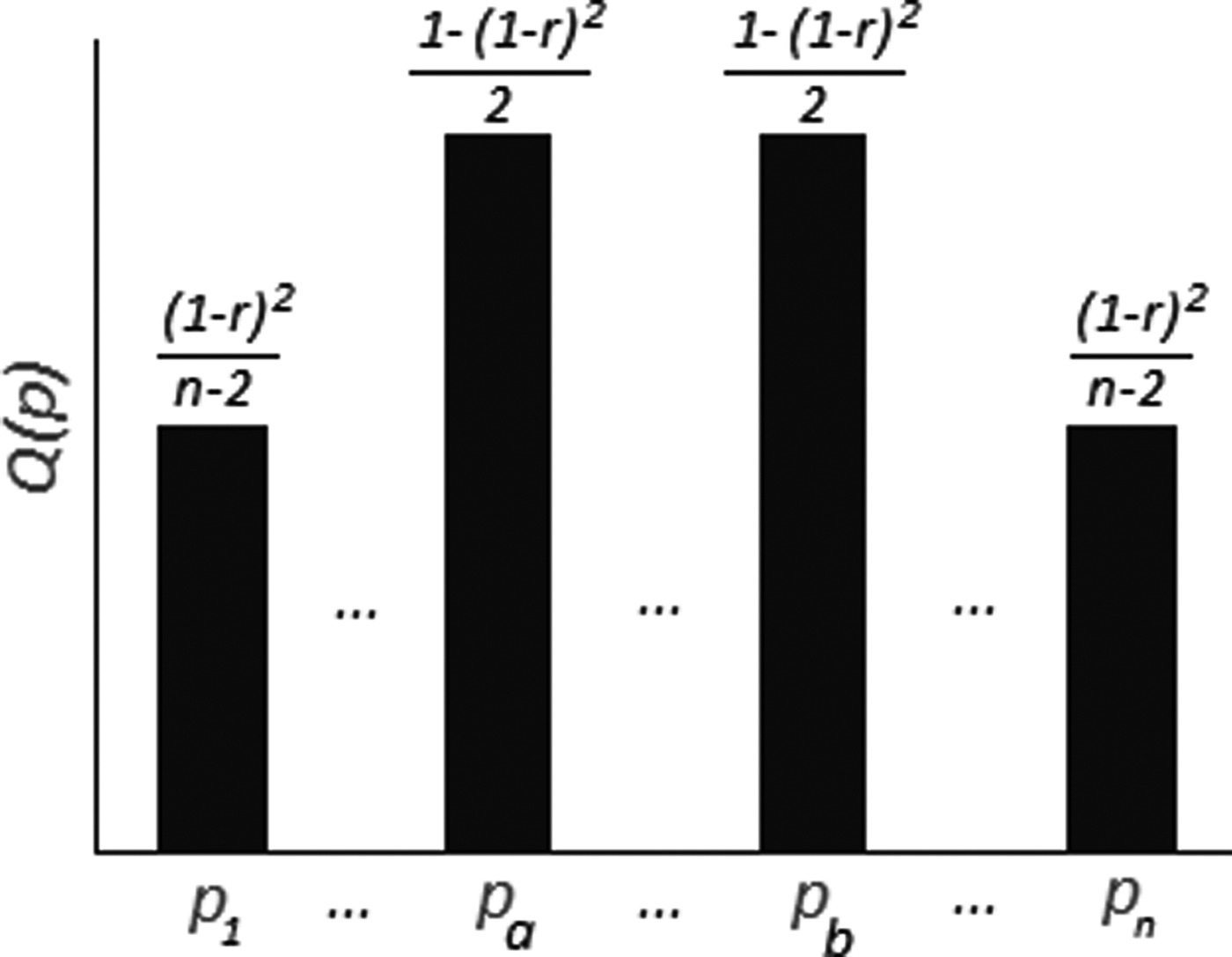
Given the supposition that a and b have a shared reliability of r, there is a probability of 1 − r that a misjudges the evidence, and similarly for b. So there is a probability of (1 − r)2 that both a and b have misjudged the evidence, and, accordingly, a probability of 1 − (1 − r)2 that one of the peers has judged the evidence correctly. That is, the likelihood that scenario (iii) obtains is (1 − r)2, and the likelihood that either scenario (i) or (ii) obtains is 1 − (1 − r)2. Moreover, given the dictum that disagreeing peers should be given equal weight regardless of whom (if any) of them actually judged the evidence correctly, we should divide the probability 1 − (1 − r)2 evenly on scenarios (i) and (ii). As such, we get the following higher-order probabilities:
 $$Q(\,p_a ) = Q(\,p_b ) = \displaystyle{{1 - (1 - r)^2} \over 2}.$$
This equation tells us that the higher-order probability of the higher-order hypothesis P(H|E) = p a is .5(1 − (1 − r)2), and similarly for P(H|E) = p b . As we should expect, the value of Q(p a ) and Q(p b ) increases when r increases – that is, the more reliable an agent is, the more likely the agent is to judge the first-order evidence correctly.
Consider, next, the remaining higher-order probabilities Q(p), for p a ≠ p ≠ p b . Given that the probability variable p is discrete and can take on n different values, there are a total of n − 2 such remaining higher-order probabilities. Thus, the likelihood of scenario (iii) – namely (1 − r)2 – should be distributed on n − 2 different higher-order probabilities. What should this distribution look like? Given our idealized model of reliability, the peers' judgments provide us with information about the value of Q(p a ) and Q(p b ), but not about the value of Q(p), for p a ≠ p ≠ p b .Footnote 11 So we need to assign prior values to Q(p), for p a ≠ p ≠ p b . One simple and intuitive way of doing this is by using the well-known Principle of Indifference (PoI) which says that, absent reasons to the contrary, one should assign equal probability to competing hypotheses.Footnote 12 By invoking PoI, we can distribute the probability (1 − r)2 evenly on each Q(p), for p a ≠ p ≠ p b :
 $$Q(\,p) = \displaystyle{{(1 - r)^2} \over {n - 2}}\;\;{\rm for} \ p_a \ne p \ne p_b. $$
As we should expect, the value of Q(p), for p a ≠ p ≠ p b , decreases when r increases: the more reliable an agent is, the less likely the agent is to misjudge the first-order evidence.
Taken together, (1) and (2) constitute the higher-order probability distribution in Peer disagreement (see Figure 1 for an illustration). If we plug this distribution into LoTP, we get the following first-order probability of H given the total evidence E T :
 $$P(H \vert E_T ) = \displaystyle{{1 - (1 - r)^2} \over 2} \cdot (\,p_a + p_b ) + (1 - r)^2 \cdot \sum\limits_{i = 1,a \ne i \ne b}^n \displaystyle{{\,p_i} \over {n - 2}}.$$
The higher-order probability distribution in Peer disagreement.

This formula dictates which credence a and b should adopt upon disagreement given that p is discrete. But since credences are typically allowed to take on any value between 0 and 1, we are really interested in the case where p is continuous in the interval [0,1]. To this end, we let n approach infinity to arrive at our formal interpretation of the variably equal weight dictum:
The Variably Equal Weight View (VEW): The parties to a peer disagreement should adopt a credence identical to the following evidential probability:
 $$P(H \vert E_T ) = \displaystyle{{1 - (1 - r)^2} \over 2} \cdot (\,p_a + p_b ) + \displaystyle{{(1 - r)^2} \over 2},$$
where H is the disputed first-order hypothesis, r is the peers' shared reliability, and E T is the peers' total evidence consisting of the first-order evidence E and the higher-order evidence given by the peers' judgments p a and p b of the evidential probability of H given E.
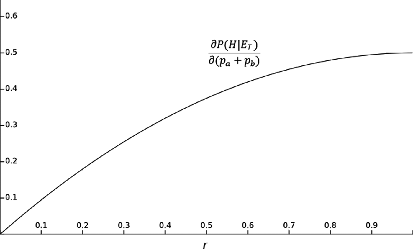
We can think of the different components of the VEW equation in terms of the scenarios (i)–(iii): the first summand (the one that features p a and p b ) corresponds to the scenarios (i) and (ii) where one of the peers has judged the evidence correctly, and the second summand (the one that doesn't feature p a and p b ) corresponds to scenario (iii) where both peers have misjudged the evidence. The relative impact or weight of these two summands on the value of P(H|E T ) depends on the relative likelihood of the scenarios (i)–(iii). These likelihoods, in turn, depend on the peers' shared reliability: high values of r leads to a high likelihood of (i) and (ii) and a low likelihood of (iii), and vice versa. Accordingly, the impact that the peers' judgments p a and p b have on the value of P(H|E T ) depends on the value of r. We may naturally depict this dependency in terms of the derivative of P(H|E T ) with respect to the sum of p a and p b (see Figure 2):
 $$\displaystyle{{\partial P(H \vert E_T )} \over {\partial (\,p_a + p_b )}} = \displaystyle{{1 - (1 - r)^2} \over 2}.$$
Intuitively, ∂P(H|E T )/∂(p a + p b ) represents the “impact factor” of p a and p b on P(H|E T ). This impact factor is solely a function of the peers' shared reliability: high values of r result in a high impact factor of p a and p b on P(H|E T ), and low values of r result in a low such impact factor. This reflects the spirit behind the variably equal weight dictum: reliable disagreeing peers should give each other equal high weight, while unreliable disagreeing peers should give each other equal low weight.
The derivative of P(H|E T ) with respect to p a + p b shows how r determines the impact of p a and p b on P(H|E T ): high values of r result in a high such impact, and vice versa.

In the extreme case where r = 0, the peers should place no weight on each other's judgments: a change in the value of p a and p b is not going to make any difference to the value of P(H|E T ). By contrast, when r = 1, the peers should place maximum weight on each other's judgments: if the average value of p a and p b changes by a given amount, the value of P(H|E T ) is going to change by the same amount. For example, if the average value of p a and p b increases by .3, the value of P(H|E T ) also increases by .3, and if the average value of p a and p b decreases by .9, the value of P(H|E T ) also decreases by .9. In between these limit cases, when 0 < r < 1, the peers should place “intermediate” weight on each other's judgments: if the value of p a and p b changes by a given amount, the value of P(H|E T ) is going to change by a somewhat smaller amount, depending on the exact value of r. For example, if r = .6 and we increase the average value of p a and p b by .3, the value of P(H|E T ) will increase by .3·.5(1 − (1 − .6)2) ≈ .13.
To illustrate VEW at work, consider a case along the lines of Weather forecasters with which we began this section:
Weather forecasters*: Two weather forecasters a and b assess the same body of meteorological data E and make private predictions of whether (H) it will rain later that day: a judges that P(H|E) = .9, and b judges that P(H|E) = .3. The weather forecasters are rationally certain that they both have a reliability of r = .7 at judging the evidence. Which credence should they adopt in H upon disagreement?
If we plug these numbers into VEW, we get the following verdict:
 $$P(H \vert E_T ) = \displaystyle{{1 - (1 -. 7)^2} \over 2}(.9 +. 3) + \displaystyle{{(1 -. 7)^2} \over 2} \approx. 59$$
So according to VEW, the weather forecasters should adopt a credence of .59 in H upon disagreement.
We now go on to explore some important consequences of VEW (§§4–5), and generalize the view to cases of non-peer disagreement (§6).
4. AGAINST SPLITTING THE DIFFERENCE
A view that has often been associated with the equal weight view is the linear averaging or “split the difference” view:Footnote 13
Split the Difference (SD): the parties to a peer disagreement should adopt a credence identical to the average, .5(p a + p b ), of their initial credences p a and p b .
An important difference between VEW and SD is that VEW takes the peers' reliability into account, whereas SD does not. Consequently, SD yields the same verdict regardless of how reliable the disagreeing peers are, whereas VEW yields different verdicts for different values of r. For example, suppose that r = .3, p a = .8, and p b = .9. According to SD, the peers should adopt a credence of .85 upon disagreement. By contrast, VEW recommends the peers to adopt a significantly lower credence of .68 because of the peers' low reliability. Since low values of r result in a low impact factor of p a and p b on P(H|E T ) the peers should only adopt a credence that is slightly higher than .5 although their judgments are quite high. This is how VEW reflects the spirit behind the variably equal weight dictum.
Although VEW generally differs from SD, there are two special cases where VEW recommends splitting the difference:
 $$P(H \vert E_T ) =. 5(\,p_a + p_b ) =. 5\ {\rm for} \ p_a + p_b = 1.$$
 $$\hskip-7.3pc \mathop {\lim} \limits_{r \to 1} P(H \vert E_T ) =. 5(p_a + p_b )$$
The former condition represents a case where the average of the peers' judgments is .5. Here, we should expect linear averaging to be the correct response: intuitively, if two peers “pull equally hard in opposite directions,” their resulting credence should not deviate from .5. The latter condition represents a limit case where the disagreeing peers are close to being perfectly reliable. Here, we should also expect linear averaging to be the correct response: when r is very high, there is a very low probability that both peers have misjudged the evidence, which means that the higher-order probability distribution Q(p) will be almost fully concentrated on the peers' judgments p a and p b . Given this – as we show in detail in a moment – linear averaging falls out as the right response. Needless to say, two perfectly reliable peers cannot really disagree (at least given The Uniqueness Thesis), so VEW will never strictly speaking recommend splitting the difference unless p a + p b = 1. But it remains true that VEW approaches SD, when r approaches 1 – that is, highly reliable disagreeing peers should approximately split the difference.
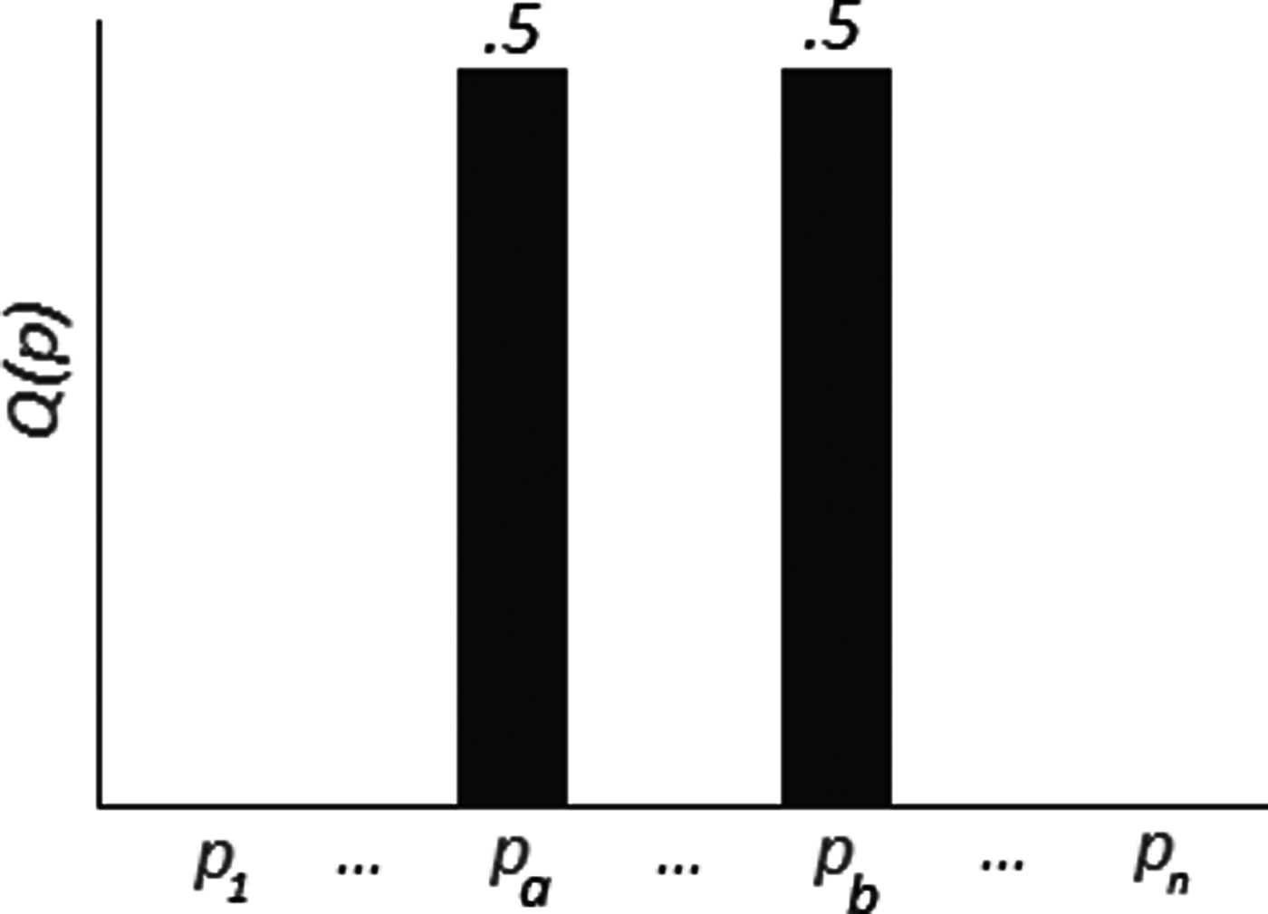
Why might one be tempted to interpret the equal weight dictum as linear averaging? We suspect that proponents of SD implicitly assume that whenever two peers a and b disagree, either (i) a has judged the evidence correctly and b hasn't, or (ii) b has judged the evidence correctly and a hasn't, but not (iii) both a and b have misjudged the evidence. Given this assumption, the equal weight dictum requires that we assign a probability of .5 to both (i) and (ii):
 $$Q(\,p_a ) = Q(\,p_b ) =. 5$$
This means that the higher-order probability distribution is fully concentrated on the peers' judgments p a and p b (see Figure 3). If we plug this distribution into LoTP, we immediately arrive at SD:
 $$P(H \vert E_T ) = p_a Q(\,p_a ) + p_b Q(\,p_b ) =. 5(\,p_a + p_b ).$$
So SD follows straightforwardly from the assumption that whenever to peers disagree, one of them must have judged the evidence correctly. The reason why SD fails is that this assumption is false: two disagreeing peers may well both have misjudged the evidence, and the likelihood of this possibility depends on how reliable the peers are.Footnote 14 , Footnote 15
The higher-order probability distribution in Peer disagreement given the assumption that, whenever two peers disagree, one of them must have judged the evidence correctly.

While we have focused our discussion on the equal weight view in this paper, note that all views of disagreement, whether conciliatory or steadfast, should take into account the possibility that two disagreeing peers may both have misjudged the evidence. To our knowledge, SD is the only quantitatively precise view of disagreement that can be shown to fail in this regard, but the mistake is one that should be avoided by all contenders in the disagreement debate.
5. SYNERGY
A desirable feature of VEW is that it gives rise to plausible instances of what Easwaran et al. (Reference Easwaran, Fenton-Glynn, Hitchcock and Velasco2016) call synergy – an effect whereby the parties to a disagreement should become more (or less) confident in the disputed proposition than any of them were prior to the disagreement. To illustrate, consider a case adapted from Christensen (Reference Christensen2009: 759) where synergy seems warranted:
Second opinion: Two doctors independently analyze the same CT scan, and they both judge that radiation will be a more effective treatment than chemotherapy. Yet, well aware that it's easy to overlook important details on CT scans, both doctors remain open to the possibility that chemotherapy is preferable to radiation: one doctor adopts a credence of .76 that radiation is preferable to chemotherapy, and the other adopts a credence of .77. To minimize the risk of conducting the wrong treatment, the doctors decide to consult each other for a second opinion. Once they learn about each other's opinions, they both increase their confidence that radiation is preferable to chemotherapy.
Here, it seems rational for the doctors to become more confident than any of them were initially. So an adequate account of peer disagreement should, it seems, give rise to synergy in some circumstances. At the same time, it is clear that synergy is not always a rational response to disagreement. For example, if the doctors in the case above had made complete opposite judgments of the CT scan, it would be irrational of them to respond synergistically to their disagreement. Thus, an adequate account of peer disagreement should give rise to synergy in some, but not all, circumstances. In the remainder of this section, we show that VEW gives rise to synergy in a restricted set of circumstances, and argue that those are circumstances in which synergy is warranted.
As a first step, we need a precise definition of synergy. Here, we take our clue from Second opinion in which synergy arises in three steps. First, the doctors independently judge the CT scan. Second, each doctor adopts what we will call her considered credence – that is, her credence upon having judged the CT scan and revised her credence in light of the possibility of having misjudged the evidence. Third, the doctors learn about each other's opinions and adopt a credence that is higher than both of their considered credences prior to disagreement.
To make this characterization precise, we need a way of determining an agent's considered credence c given that the agent has a reliability of r and has judged that P(H|E) = j. By reapplying, mutatis mutandis, the procedure used in
 ${\rm \S}$
3 to derive VEW, we arrive at the following simple relationship between c, j, and r:
 $$c = r \cdot j + \displaystyle{{1 - r} \over 2}.$$
This formula says how a single agent should take her own fallibility into account, much like VEW says how two disagreeing peers should take their fallibility jointly into account. As we should expect, c gets closer and closer to j as r approaches 1. This reflects that a reliable agent is likely to judge the evidence correctly, whereas an unreliable agents is unlikely to do so. Given this way of determining an agent's considered credence prior to disagreement, we can go on to define synergy as follows:
Synergy: a case of peer disagreement gives rise to synergy iff
 $P(H\midE_T) \notin [c_{min},c_{max}]$
, where c
min
is the considered credence of the least confident peer, and c
max
is the considered credence of the most confident peer.
If we use VEW and (5) to substitute expressions for P(H|E T ), c min , and c max in this definition, we get the following expression:
 $$\displaystyle{{1 - (1 - r)^2} \over 2}(\,j_{min} + j_{max} ) + \displaystyle{{(1 - r)^2} \over 2}\ {\notin} \ \left[ {r \cdot j_{min} + \displaystyle{{1 - r} \over 2},r \cdot j_{max} + \displaystyle{{1 - r} \over 2}} \right].$$
This double inequality has two solutions which correspond to the conditions under which VEW gives rise to synergy (we omit the formal details):
Synergy conditions: VEW gives rise to synergy iff either
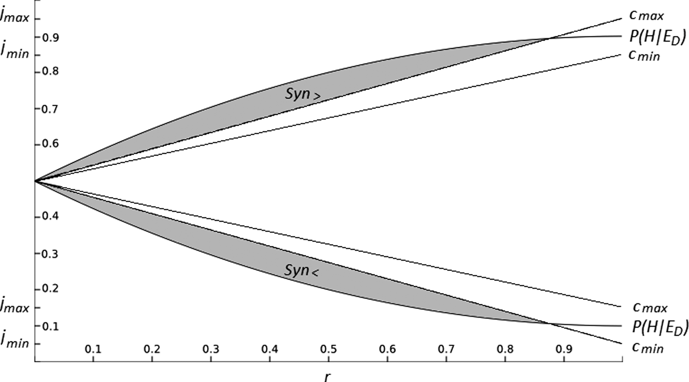
 $$\quad {\rm Syn}_ \lt : j_{max} \lt. 5 \ {\rm and} \ r \lt \displaystyle{{2j_{max} - 1} \over {\,j_{max} + j_{min} - 1}};{\rm or}$$
 $${\rm Syn}_ \gt : j_{min} \gt. 5 \ {\rm and}\ r \lt \displaystyle{{2j_{min} - 1} \over {j_{max} + j_{min} - 1}}.$$
Here, Syn < represents the conditions under which the peers should both revise their considered credences downwards (i.e. P(H|E T ) < c min ). Conversely, Syn > represents the conditions under which the peers should boost each other's considered credences upwards (i.e. P(H|E T ) > c max ).
It is easily verified that the values of (2j max − 1)/(j min + j max − 1) and (2j max − 1)/(j min + j max − 1) both increase when the value of j max − j min decreases. The value of j max − j min intuitively represents the extent to which the peers disagree: when j max − j min is high, the peers disagree to a high extent, and vice versa. We can thus think of VEW as giving rise to synergy under two broad sets of circumstances: either when both peers make judgments lower than .5 and their shared reliability is sufficiently low compared with the extent to which they disagree, or when both peers make judgments higher than .5 and their shared reliability is sufficiently low compared with the extent to which they disagree. Equivalently, VEW does not give rise to synergy when .5 ∈ [j min , j max ], or when the peers have a high reliability compared with the extent to which they disagree (Figure 4).
The shaded areas mark the conditions under which VEW gives rise to synergy. The upper part of the graph illustrates a case where j min = .85 and j max = .95, while the lower part of the graph illustrates a case where j min = .05 and j max = .15.

To motivate that Synergy conditions successfully tracks the circumstances under which synergy is intuitively warranted, consider the following four variations of Weather forecasters:
Weather forecasters**: Two weather forecasters with a shared reliability of r = .8 independently analyze the same body of meteorological data, and form judgments of the evidential probability that it will rain later today.
(a) Let j
min
= .7 and j
max
= .71. Then c
min
= .66 and c
max
= .67. Here, VEW gives rise to synergy: the weather forecasters should adopt credence .7 upon disagreement, and
 $.7{\ \notin}\ [.66,\!.67]$
.
(b) Let j
min
= .29 and j
max
= .3. Then c
min
= .33 and c
max
= .34. Here, VEW gives rise to synergy: the weather forecasters should adopt credence .3 upon disagreement, and
 $.3\ {\notin}\ [.33,\!.34]$
.
(c) Let j min = .3 and j max = .8. Then c min = .34 and c max = .74. Here, VEW doesn't give rise to synergy: the weather forecasters should adopt credence .55 upon disagreement, and .55 ∈ [.34,.74].
(d) Let j min = .51 and j max = .99. Then c min = .59 and c max = .86. Here, VEW doesn't give rise to synergy: the weather forecasters should adopt credence .74 upon disagreement, and .74 ∈ [.59,.86].
The first two cases (a) and (b) represent situations like Second opinion where two reliable peers only disagree to a small extent. In such cases, synergy seems warranted as two peers are less likely to be mistaken than is either one of them. The third case (c) represents situations where two peers make judgments on opposite sides of .5. In such cases, synergy does not seem warranted: if two peers pull in opposite directions, they should end up with a credence somewhere in the interval between their initial credences. Finally, case (d) represents situations where two peers have a high shared reliability compared with the extent to which they disagree. In such cases, synergy also does not seem warranted: if I have a high considered credence of .99 in H and learn that my peer has a much lower considered credence of .51 in H, it seems that I should lower my confidence in H (and my peer should increase his). In sum, then, VEW seems to give rise to synergy under the right set of circumstances. It is also worth noting that VEW gives rise to synergy in cases of peer agreement. If j min = j max = j, VEW reduces to the following view:
 $$P(H \vert E_T ) = (1 - (1 - r)^2 ) \cdot j + \displaystyle{{(1 - r)^2} \over 2}.$$
It is easy to see that P(H|E T ) < c when c < .5, and P(H|E T ) > c when c > .5, where c = r ċ j + .5(1 − r) is the peers' shared considered credence prior to disagreement. As such, VEW always gives rise to synergy in cases of peer agreement (except when c = .5): if the peers start out with a considered credence higher than .5, they should boost each other's considered credences upwards, and if they start out with a considered credence lower than .5, they should boost each other's considered credences downwards. For example, if r = .6 and c = .7, then P(H|E T ) = .78, and if r = .6 and c = .2, then P(H|E T ) = .08.
Let us close our discussion of synergy with a brief comparison to Easwaran et al. (Reference Easwaran, Fenton-Glynn, Hitchcock and Velasco2016) who have proposed a heuristic, called Upco, for how to update one's credence upon learning the credence of another agent. If c a and c b represent the initial credences of two agents a and b, Upco recommends the agents to adopt the following posterior credence:
 $$\quad c_a^ + = c_b^ + = \displaystyle{{c_a c_b} \over {c_a c_b + (1 - c_a )(1 - c_b )}}$$
Upco is designed to mimic Bayesian conditionalization in cases where it is reasonable to suppose that agents have truth-tracking credences – that is, when agents are likely to have high credences in truths and low credences in falsehoods. By combining a formally precise version of this assumption with Bayes' theorem, Easwaran et al. show that Upco falls out as the resulting update rule.
There are two important differences between VEW and Upco. First, VEW is derived from an evidence-based notion of reliability, whereas Upco is derived from a truth-based notion of reliability. Second, VEW is supposed to apply in all cases of peer disagreement, regardless of how reliable the peers are, whereas Upco is only supposed to apply in cases where agents are expected to be reliable (in the truth-based sense). Despite these differences, however, we can draw a few lines of comparison between VEW and Upco in relation to synergy. First, Upco agrees with VEW that synergy should not arise when two agents initially “pull in opposite directions”: it is easily shown that
 $c_a^ + = c_b^ + \in [c_a, c_b ]$
when c
a
≤ .5 ≤ c
b
. Second, Upco agrees with VEW that synergy should arise when two reliable agents only disagree to a small extent. For example, if c
a
= .7 and c
b
= .71, Upco recommends that the agents adopt a credence
 $c_a^ + = c_b^ + \approx. 85$
upon disagreement. But third, Upco seems to disagree with VEW when it comes to cases where two reliable agents with initial credences on the same side of .5 disagree to a high extent. For while we have seen that VEW does not give rise to synergy in such cases, it is easily verified that Upco gives rise to synergy whenever
 $.5\ \notin \ [c_a, c_b ]$
. For example, if c
a
= .99 and c
b
= .51, Upco yields a posterior credence slightly higher than .99. This result makes sense given the assumption that agents have truth-tracking credences. For given this assumption, even credences that are only slightly higher than .5 should be taken as a slight indication that the relevant proposition is true rather than false. At the same time, however, it seems clear that two disagreeing peers with initial considered credences .99 and .51 respectively should not respond synergistically to their disagreement. Rather, when the most confident peer learns that her peer is much less confident than herself, this should be taken as an indication that her own judgment of the evidence was too optimistic to begin with. So for the purposes of capturing the conditions under which synergy should arise in paradigmatic cases peer disagreement, VEW seems to be superior to Upco.
6. NON-PEER DISAGREEMENT
So far we have restricted our attention to idealized cases of disagreement between epistemic peers who, by stipulation, share all of their relevant evidence and are equally reliable at judging that evidence. The benefit of such idealizations is that they make a precise analysis considerably more tractable. Yet, the interest of idealized cases of disagreement largely derives from the light they may shed on disagreement more generally. As such, it is worthwhile exploring how VEW may be generalized to cases of non-peer disagreement. Here, we will focus on three central weakenings of idealizations that are often assumed in discussions of peer disagreement:
Reliability non-peerhood: Two agents are reliability non-peers (on a given occasion) with respect to a batch of evidence E bearing on a hypothesis H iff (on that occasion) they are not equally likely to judge E correctly.
n-party disagreement: A disagreement is an n-party disagreement iff there are n parties to the disagreement.
Evidential non-peerhood: Two agents are evidential non-peers (on a given occasion) with respect to a hypothesis H iff (on that occasion) they do not possess the same total body of evidence bearing on H.
We begin by implementing the first two generalizations. Let a 1, …, a n be n different evidential peers with (possibly different) reliabilities r 1, …, r n . On a given occasion, the agents make (possibly different) judgments p 1, …, p n of the evidential probability of H given E. Given this, we can reapply, mutatis mutandis, the procedure from §3 to arrive at the following generalization of VEW (we omit the formal details):
 $$P(H \vert E_T ) = \left( {1 - \prod\limits_{i = 1}^n 1 - r_i} \right)\displaystyle{{\sum\nolimits_{i = 1}^n {\,p_i r_i}} \over {\sum\nolimits_{i = 1}^n {r_i}}} +. 5\left( {\prod\limits_{i = 1}^n 1 - r_i} \right).$$
As we should expect, (6) reduces to VEW when n = 2 and r 1 = r 2. Moreover, it is easily verified that (6) recommends the agents to adopt a credence identical to the average of their judgments under two special circumstances: when the average of their judgments is .5, or when r 1 =ċċċ= r n → 1. Under these conditions, (6) in effect reduces to a generalized version of SD.
Like VEW, (6) is based on our idealized notion of reliability according to which an agent has a reliability of r just in case there is a probability of r that the agent makes a perfect judgment of the evidence. But as previously mentioned, agents like you and I presumably rarely (if ever) judge evidence so precisely. It seems more reasonable to think of an agent's reliability as the likelihood that the agent's judgment will at least be “in the right ballpark.” A natural way to make this idea precise is to model an agent's reliability in terms of a more or less spread-out higher-order probability distribution. Suppose that agent a judges that P(H|E) = p
a
on a given occasion. We can then let σ
a
(p) be a higher-order probability function representing what we will call a’s reliability distribution on the given occasion. On this model, a has a high reliability just in case the value of σ
a
(p) is high for values of p close to p
a
, and low for values of p far from p
a
. Given that the probability variable p is continuous, σ
a
is a density function which should be normalized as usual (
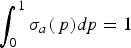 $\int_0^1 \sigma _a (\,p)dp = 1$
).
Given this setup, we can then use LoTP to calculate the first-order probability of H given the conjunction of the first-order evidence E and the higher-order evidence E a given by a’s judgment:
 $$P(H \vert E_a ) = \int_0^1 p \cdot \sigma _a (\,p) dp.$$
This equation yields an agent's considered credence given our new model of reliability, just as (5) yields an agent's considered credence given the old model of reliability.
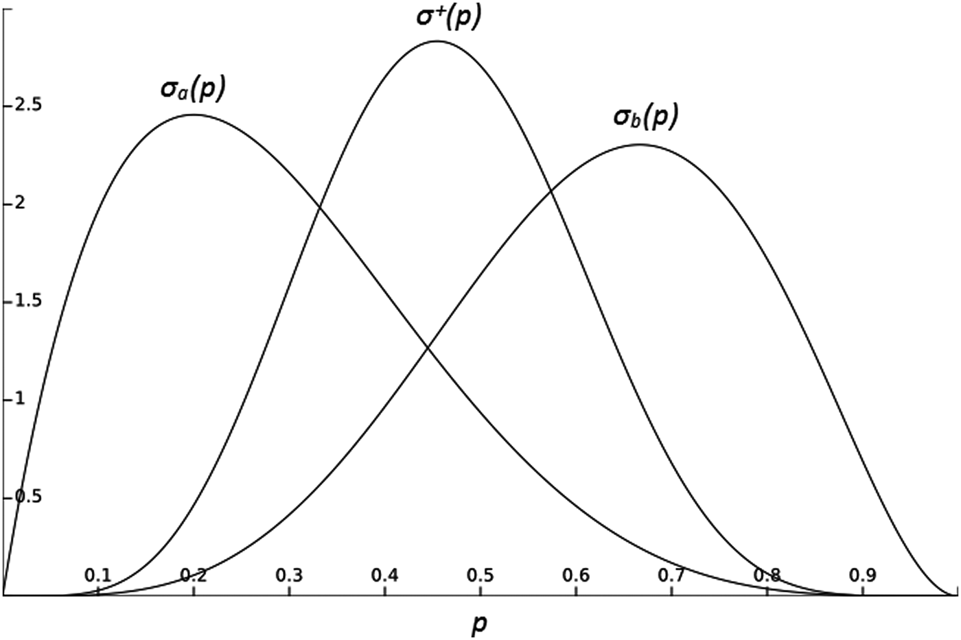
Suppose, next, that n different evidential peers a 1, …, a n have (possibly different) reliability distributions σ 1, …, σ n on a given occasion. To determine which credence the agents should adopt upon disagreement, we need to combine σ 1, …, σ n to arrive at a final higher-order probability distribution which we can call σ +. Given σ +, we can use LoTP to determine P(H|E T ), where, as usual, E T is the total body of evidence consisting of the conjunction of E and all of the agents' judgments:
 $$P(H \vert E_T ) = \int_0^1 p \cdot \sigma ^ + (\,p) dp.$$
The combined higher-order probability distribution σ + is obtained by normalizing the product of σ 1, …, σ n :
 $$\sigma ^ + (\,p) = \displaystyle{{\prod\nolimits_{i = 1}^n {\sigma _i (\,p)}} \over {\int_0^1 \prod\nolimits_{i = 1}^n {\sigma _i (\,p)} dp}}.$$
By substitution in (8), we arrive at the following generalization of VEW:
 $$P(H \vert E_T ) = \int_0^1 p \cdot \displaystyle{{\prod\nolimits_{i = 1}^n {\sigma _i (\,p)}} \over {\int_0^1 \prod\nolimits_{i = 1}^n {\sigma _i (\,p)} dp}} dp.$$
To illustrate this view, suppose that n = 2, and suppose that the two agents' reliability distributions are given by the following normalized beta distributions (see Figure 5):
 $$\sigma _a (\,p) = 30 \cdot p \cdot (1 - p)^4 $$
 $$\sigma _b (p) = 105 \cdot p^4 \cdot (1 - p)^2. $$
If we plug these reliability distributions into (7), we get a and b’s considered credences prior to disagreement:
 $$P(H \vert E_a ) = \int_0^1 p \cdot 30 \cdot p \cdot (1 - p)^4 dp \approx. 29$$
 $$P(H \vert E_b ) = \int_0^1 p \cdot 105 \cdot p^4 \cdot (1 - p)^2 dp \approx. 63.$$
If, instead, we plug the reliability distributions into (9), we get the credence that a and b should adopt upon disagreement:
 $$P(H \vert E_T ) = \int_0^1 p \cdot \displaystyle{{30 \cdot p \cdot (1 - p)^4 \cdot 105 \cdot p^4 \cdot (1 - p)^2} \over {\int_0^1 30 \cdot p \cdot (1 - p)^4 \cdot 105 \cdot p^4 \cdot (1 - p)^2 dp}} dp \approx. 46$$
Note that a and b should not respond synergistically to their disagreement (.46 ∈ [.29,.63]) which was to be expected since a and b initially pull in opposite directions. While VEW generalizes quite straightforwardly to cases of disagreement between n agents with (possibly) different reliabilities, it is less clear how to generalize VEW to disagreements between evidential non-peers. As Christensen (Reference Christensen2007: 211–12) notes, we may reasonably suppose that evidential parity produces the same results as evidential peerhood: it doesn't seem to make a difference whether the disagreeing parties have the same evidence, or whether they have different, but equally good, evidence. But what happens when the disagreeing parties do not possess equally good evidence? To answer this question, we need a quantitative measure of the relative quality of different bodies of evidence. This measure should influence the weight that should be placed on the opinions of different agents: the better an agent's evidence, the more weight should (other things being equal) be placed on the agent's opinion. We are optimistic that our framework can eventually be generalized to capture this idea. But we leave a detailed investigation for future work.
The reliability distributions of two agents a and b on a given occasion of disagreement.

7. CONCLUSION
We have outlined a simple formal framework for reasoning about the evidential impact of a body of higher-order evidence, and have used this framework to motivate a novel interpretation of the equal weight view of disagreement – we have called it the Variably Equal Weight View (VEW). According to VEW, disagreeing peers should always place equal weight on each other's opinions, but the amount of weight they should give each other depends on how reliable they are: roughly, reliable peers should give each other equal high weight, while unreliable peers should give each other equal low weight. We showed that VEW differs considerably from the standard Split the Difference (SD) interpretation of the equal weight view, and showed that VEW gives rise to plausible instances of synergy. Lastly, we explored how VEW may be generalized to cases of non-peer disagreement.Footnote 16