2.1 Space–time integral method

We consider a PIV velocity field $\tilde{\boldsymbol{v}}$ , which is a measurement of an actual velocity field $\boldsymbol{v}$ , at evenly distributed time instances $t_{i}=i\unicode[STIX]{x0394}t$ , where $i=1,2,3,\ldots ,$ and $\unicode[STIX]{x0394}t$ is the sampling time. We construct an improved velocity field $\boldsymbol{u}$ , by minimising the difference between $\boldsymbol{u}$ and $\tilde{\boldsymbol{v}}$ under the constraint that $\boldsymbol{u}$ satisfies the Navier–Stokes equations,

(2.1) $$\begin{eqnarray}\displaystyle \boldsymbol{R}(\boldsymbol{w})=\left(\begin{array}{@{}c@{}}\unicode[STIX]{x2202}_{t}\boldsymbol{u}+\boldsymbol{u}\boldsymbol{\cdot }\unicode[STIX]{x1D735}\boldsymbol{u}+\unicode[STIX]{x1D735}p-\unicode[STIX]{x1D708}\unicode[STIX]{x1D6FB}^{2}\boldsymbol{u}\\ \unicode[STIX]{x1D735}\boldsymbol{\cdot }\boldsymbol{u}\end{array}\right)=\mathbf{0}, & & \displaystyle\end{eqnarray}$$

where $\boldsymbol{w}=(\boldsymbol{u},p)$ is referred to as the ‘state variable’, $p$ is the fluid pressure and $\unicode[STIX]{x1D708}$ is the fluid kinematic viscosity. We therefore minimise a constrained cost functional, referred to as the Lagrangian $\mathscr{L}$ ,

(2.2) $$\begin{eqnarray}\displaystyle \mathscr{L}=\int _{t_{1}}^{t_{P}}\left(\frac{1}{2}\Vert \boldsymbol{u}-\tilde{\boldsymbol{v}}\Vert ^{2}\mathop{\sum }_{i=1}^{P}\unicode[STIX]{x1D6FF}(t-t_{i})+\langle \hat{\boldsymbol{w}},\boldsymbol{R}(\boldsymbol{w})\rangle \right)\text{d}t, & & \displaystyle\end{eqnarray}$$

which involves a set of $P$ measurements, taken from an assimilation window $t_{1}<t<t_{P}$ , where $\unicode[STIX]{x1D70F}=t_{P}-t_{1}$ is the assimilation time. The Lagrange multiplier $\hat{\boldsymbol{w}}=(\hat{\boldsymbol{u}},\hat{p})$ is introduced to enforce the constraint (2.1). Note, that a hat $\hat{~}$ above a field variable denotes, that the field variable is a Lagrange multiplier. In (2.2) time integration is performed from the first to the last ( $P$ th) measurement, $\unicode[STIX]{x1D6FF}(\cdot )$ denotes the Dirac delta function and $\Vert \cdot \Vert$ is the norm based on the standard inner product $\langle \cdot ,\cdot \rangle$ , which, when applied to two complex vector fields $\boldsymbol{a}$ and $\boldsymbol{b}$ , reads

(2.3) $$\begin{eqnarray}\displaystyle \langle \boldsymbol{a},\boldsymbol{b}\rangle =\int \text{d}V\boldsymbol{a}^{\ast }\boldsymbol{\cdot }\boldsymbol{b}. & & \displaystyle\end{eqnarray}$$

Here $V$ is the spatial domain, on which $\boldsymbol{a}$ and $\boldsymbol{b}$ are defined, and the superscript $^{\ast }$ denotes complex conjugation.

The goal is to find $\boldsymbol{u}$ , that minimises $\mathscr{L}$ (2.2). Since $\boldsymbol{u}$ is determined by its initial conditions $\boldsymbol{u}_{1}$ , we determine $\boldsymbol{u}$ by minimising $\mathscr{L}$ with respect to $\boldsymbol{u}_{1}$ . It is noted, that subscript indices refer to time instances, e.g. $\boldsymbol{u}_{1}=\boldsymbol{u}(t_{1})$ . To minimise $\mathscr{L}$ with respect to $\boldsymbol{u}_{1}$ , we need the gradient of $\mathscr{L}$ with respect to $\boldsymbol{u}_{1}$ , i.e. $\unicode[STIX]{x1D6FF}\mathscr{L}/\unicode[STIX]{x1D6FF}\boldsymbol{u}_{1}$ . To derive an expression for $\unicode[STIX]{x1D6FF}\mathscr{L}/\unicode[STIX]{x1D6FF}\boldsymbol{u}_{1}$ we start by writing the variation of the cost functional $\unicode[STIX]{x1D6FF}\mathscr{L}$ due to an infinitesimal variation of the state variable $\unicode[STIX]{x1D6FF}\boldsymbol{w}=(\unicode[STIX]{x1D6FF}\boldsymbol{u},\unicode[STIX]{x1D6FF}p)$ ,

(2.4) $$\begin{eqnarray}\displaystyle \unicode[STIX]{x1D6FF}\mathscr{L}=\int _{t_{1}}^{t_{P}}\left(\langle \boldsymbol{u}-\tilde{\boldsymbol{v}},\unicode[STIX]{x1D6FF}\boldsymbol{u}\rangle \mathop{\sum }_{i=1}^{P}\unicode[STIX]{x1D6FF}(t-t_{i})+\langle \hat{\boldsymbol{w}},\unicode[STIX]{x1D6FF}\boldsymbol{R}(\boldsymbol{w})\rangle \right)\text{d}t. & & \displaystyle\end{eqnarray}$$

We rewrite the Lagrange multiplier term in (2.4) using integration by parts (e.g. Gunzburger Reference Gunzburger2003),

(2.5) $$\begin{eqnarray}\displaystyle \unicode[STIX]{x1D6FF}\mathscr{L}=\int _{t_{1}}^{t_{P}}\left(\langle \boldsymbol{u}-\tilde{\boldsymbol{v}},\unicode[STIX]{x1D6FF}\boldsymbol{u}\rangle \mathop{\sum }_{i=1}^{P}\unicode[STIX]{x1D6FF}(t-t_{i})+\langle \hat{\boldsymbol{R}}(\boldsymbol{w},\hat{\boldsymbol{w}}),\unicode[STIX]{x1D6FF}\boldsymbol{w}\rangle \right)\text{d}t+\langle \hat{\boldsymbol{u}}_{P},\unicode[STIX]{x1D6FF}\boldsymbol{u}_{P}\rangle -\langle \hat{\boldsymbol{u}}_{1},\unicode[STIX]{x1D6FF}\boldsymbol{u}_{1}\rangle , & & \displaystyle \nonumber\\ \displaystyle & & \displaystyle\end{eqnarray}$$

where $\hat{\boldsymbol{R}}$ is the adjoint of the linearised Navier–Stokes equations $\boldsymbol{R}$ (2.1),

(2.6) $$\begin{eqnarray}\displaystyle \hat{\boldsymbol{R}}(\boldsymbol{w},\hat{\boldsymbol{w}})=\left(\begin{array}{@{}c@{}}-\unicode[STIX]{x2202}_{t}\hat{\boldsymbol{u}}-\boldsymbol{u}\boldsymbol{\cdot }(\unicode[STIX]{x1D735}\hat{\boldsymbol{u}}+\unicode[STIX]{x1D735}\hat{\boldsymbol{u}}^{\text{T}})-\unicode[STIX]{x1D735}\hat{p}-\unicode[STIX]{x1D708}\unicode[STIX]{x1D6FB}^{2}\hat{\boldsymbol{u}}\\ -\unicode[STIX]{x1D735}\boldsymbol{\cdot }\hat{\boldsymbol{u}}\end{array}\right), & & \displaystyle\end{eqnarray}$$

where a hat $\hat{~}$ above an operator denotes the adjoint of the linearised version of that operator, and $\unicode[STIX]{x1D735}\hat{\boldsymbol{u}}^{\text{T}}$ is the transpose of $\unicode[STIX]{x1D735}\hat{\boldsymbol{u}}$ . In (2.5) the terms involving $\hat{\boldsymbol{u}}_{P}$ and $\hat{\boldsymbol{u}}_{1}$ are time-boundary terms, that are obtained by integrating by parts the time derivative term in $\langle \hat{\boldsymbol{w}},\unicode[STIX]{x1D6FF}\boldsymbol{R}(\boldsymbol{w})\rangle$ in (2.4). These terms determine the initial and final conditions for $\hat{\boldsymbol{u}}$ at $t=t_{P}$ and at $t=t_{1}$ , respectively. We do not consider similar spatial boundary terms, as we assume spatial periodicity, for simplicity.

We find the initial value $\boldsymbol{u}_{1}$ that minimises the cost functional $\mathscr{L}$ (2.2), using a conjugate gradient method, by iteratively updating $\boldsymbol{u}_{1}$ in a search direction, that is related to the functional derivative of $\mathscr{L}$ with respect to $\boldsymbol{u}_{1}$ . From (2.5) we find that

(2.7) $$\begin{eqnarray}\displaystyle \frac{\unicode[STIX]{x1D6FF}\mathscr{L}}{\unicode[STIX]{x1D6FF}\boldsymbol{u}_{1}}=-\hat{\boldsymbol{u}}_{1}. & & \displaystyle\end{eqnarray}$$

To find the Lagrange multiplier $\hat{\boldsymbol{u}}_{1}$ at instant $t_{1}$ , we use the equation of motion for $\hat{\boldsymbol{u}}$ . This equation is derived from (2.5), by demanding that the Lagrangian $\mathscr{L}$ is at an extremum with respect to the state variable $\boldsymbol{w}$ , i.e. $\unicode[STIX]{x1D6FF}\mathscr{L}$ is zero under infinitesimal variation $\unicode[STIX]{x1D6FF}\boldsymbol{w}$ ,

(2.8a ) $$\begin{eqnarray}\displaystyle \left.\begin{array}{@{}c@{}}-\unicode[STIX]{x2202}_{t}\hat{\boldsymbol{u}}-\boldsymbol{u}\boldsymbol{\cdot }(\unicode[STIX]{x1D735}\hat{\boldsymbol{u}}+\unicode[STIX]{x1D735}\hat{\boldsymbol{u}}^{\text{T}})-\unicode[STIX]{x1D735}\hat{p}-\unicode[STIX]{x1D708}\unicode[STIX]{x1D6FB}^{2}\hat{\boldsymbol{u}}+(\boldsymbol{u}-\tilde{\boldsymbol{v}})\displaystyle \mathop{\sum }_{i=1}^{P}\unicode[STIX]{x1D6FF}(t-t_{i})=\mathbf{0},\\ -\unicode[STIX]{x1D735}\boldsymbol{\cdot }\hat{\boldsymbol{u}}=\mathbf{0}.\end{array}\right\} & & \displaystyle\end{eqnarray}$$

According to (2.8a ), the Lagrange multiplier $\hat{\boldsymbol{u}}$ is incompressible and is advected by $\boldsymbol{u}$ and is subjected to a (negative) viscosity $-\unicode[STIX]{x1D708}$ and is driven by a source term, which is the difference between the measurement $\tilde{\boldsymbol{v}}$ and the reconstruction $\boldsymbol{u}$ , at discrete sampling times $t_{i}$ . Due to the negative viscosity, the equation is integrated backward in time. The corresponding ‘initial’ conditions at time $t_{P}$ and ‘final’ conditions at time $t_{1}$ are found from (2.5), by demanding that $\unicode[STIX]{x1D6FF}\mathscr{L}$ is zero under infinitesimal variations $\unicode[STIX]{x1D6FF}\boldsymbol{u}_{P}$ and $\unicode[STIX]{x1D6FF}\boldsymbol{u}_{1}$ , giving

(2.8b ) $$\begin{eqnarray}\displaystyle \hat{\boldsymbol{u}}_{P}=\mathbf{0}, & & \displaystyle\end{eqnarray}$$

and

(2.8c ) $$\begin{eqnarray}\displaystyle \hat{\boldsymbol{u}}_{1}=\mathbf{0}. & & \displaystyle\end{eqnarray}$$

The conjugate gradient update direction $\hat{\boldsymbol{u}}_{1}$ (2.7) is found by integrating (2.8a ) backward in time, using ‘initial’ conditions given by (2.8b ). After updating the initial conditions for the forward problem $\boldsymbol{u}_{1}$ , equation (2.1) is integrated (forward in time), which gives a new source term for the Lagrange multiplier equation (2.8a ). This procedure is repeated until $\mathscr{L}$ is at an extremum, with respect to $\boldsymbol{u}_{1}$ , which, according to (2.7), corresponds to (2.8c ) being satisfied, to a certain degree of accuracy.

2.2 Space integral method

In this work we compare the performance of the STIM (2.2) to a SIM, which is similar to previously used methods, to improve PIV data (e.g. Ruhnau et al. Reference Ruhnau, Kohlberger, Schnörr and Nobach2005). The SIM minimises, at each instant $t=t_{i}$ , the following cost functional, which penalises the difference between the reconstruction $\boldsymbol{u}$ and the measurement $\tilde{\boldsymbol{v}}$ , under the constraint that $\boldsymbol{u}$ is divergence free

(2.9) $$\begin{eqnarray}\displaystyle \mathscr{L}={\textstyle \frac{1}{2}}\Vert \boldsymbol{u}-\tilde{\boldsymbol{v}}\Vert ^{2}+\langle \hat{p},\unicode[STIX]{x1D735}\boldsymbol{\cdot }\boldsymbol{u}\rangle +{\textstyle \frac{1}{2}}\unicode[STIX]{x1D705}\Vert \unicode[STIX]{x1D6FB}^{2}\boldsymbol{u}\Vert ^{2}, & & \displaystyle\end{eqnarray}$$

and where a regularisation term $\unicode[STIX]{x1D705}\Vert \unicode[STIX]{x1D6FB}^{2}\boldsymbol{u}\Vert ^{2}$ is added to suppress the noise at large wavenumbers (e.g. Tikhonov & Arsenin Reference Tikhonov and Arsenin1977). Here $\unicode[STIX]{x1D705}$ is referred to as the regularisation strength. Minimising $\mathscr{L}$ with respect to $\boldsymbol{u}$ involves computing the variation of $\mathscr{L}$ due to a variation in $\boldsymbol{u}$

(2.10) $$\begin{eqnarray}\displaystyle \unicode[STIX]{x1D6FF}\mathscr{L}=\langle \boldsymbol{u}-\tilde{\boldsymbol{v}},\unicode[STIX]{x1D6FF}\boldsymbol{u}\rangle -\langle \unicode[STIX]{x1D735}\hat{p},\unicode[STIX]{x1D6FF}\boldsymbol{u}\rangle +\langle \unicode[STIX]{x1D705}\unicode[STIX]{x1D6FB}^{4}\boldsymbol{u},\unicode[STIX]{x1D6FF}\boldsymbol{u}\rangle , & & \displaystyle\end{eqnarray}$$

where we have applied integration by parts. To find the reconstructed velocity field $\boldsymbol{u}$ , we demand that $\unicode[STIX]{x1D6FF}\mathscr{L}$ is zero under infinitesimal variation $\unicode[STIX]{x1D6FF}\boldsymbol{u}$

(2.11) $$\begin{eqnarray}\displaystyle (1+\unicode[STIX]{x1D705}\unicode[STIX]{x1D6FB}^{4})\boldsymbol{u}=\tilde{\boldsymbol{v}}+\unicode[STIX]{x1D735}\hat{p}. & & \displaystyle\end{eqnarray}$$

Here the term $\unicode[STIX]{x1D735}\hat{p}$ ensures that $\boldsymbol{u}$ is divergence free

(2.12) $$\begin{eqnarray}\displaystyle \unicode[STIX]{x1D735}\boldsymbol{\cdot }\boldsymbol{u}=\mathbf{0}. & & \displaystyle\end{eqnarray}$$

The solution to (2.11), (2.12) in Fourier space reads

(2.13) $$\begin{eqnarray}\displaystyle \boldsymbol{u}^{\boldsymbol{k}}=\frac{\tilde{\boldsymbol{v}}^{\boldsymbol{k}}}{1+\unicode[STIX]{x1D705}k^{4}}\boldsymbol{\cdot }\left(\unicode[STIX]{x1D739}-\frac{\boldsymbol{k}\boldsymbol{k}}{k^{2}}\right), & & \displaystyle\end{eqnarray}$$

where the superscript indices refer to the wavevectors of the spatial Fourier modes. Equation (2.13) shows, that the regularisation term in the cost functional (2.9) effectively applies hyper diffusion to the measurement field $\tilde{\boldsymbol{v}}$ . The order of the hyper diffusion, which in this case equals four, depends on the exponent on the velocity gradient in the $\unicode[STIX]{x1D705}$ -term in (2.9), which in this case equals two. For a unit exponent we would have recovered normal, second-order diffusion (see e.g. Ruhnau et al. Reference Ruhnau, Kohlberger, Schnörr and Nobach2005). Fourth-order diffusion is chosen above second-order diffusion however, since the former affects more selectively the large wavenumbers, while leaving the small wavenumbers intact.

3.1 General considerations

In this work we study the performance of the STIM (2.2) to improve the accuracy of synthetic PIV data. Before considering 2-D turbulent flow cases in § 4, we start in this section by considering one-dimensional (1-D) linear problems, for which analytical expressions can be derived for the method performance. In general, the linear equation of motion reads

(3.1) $$\begin{eqnarray}\displaystyle \unicode[STIX]{x2202}_{t}u-S(u)=0, & & \displaystyle\end{eqnarray}$$

where $S$ is a linear spatial operator. We decompose the spatial part of $u$ into the Fourier modes $\exp (\unicode[STIX]{x1D55A}kx)$ , where $k$ is the wavenumber and where $\unicode[STIX]{x1D55A}=\sqrt{-1}$ ,

(3.2) $$\begin{eqnarray}\displaystyle u=u^{k}(t)\exp (\unicode[STIX]{x1D55A}kx). & & \displaystyle\end{eqnarray}$$

Here $u^{k}(t)$ are the time-dependent Fourier coefficients, and summation of repeated indices is assumed. It is noted, that superscript indices refer to Fourier coefficients. Inserting (3.2) into (3.1) and taking the inner product (2.3) of the result with $\exp (\unicode[STIX]{x1D55A}lx)$ and using the orthogonality property of $\exp (\unicode[STIX]{x1D55A}kx)$ , gives the equation of motion of $u^{l}$

(3.3) $$\begin{eqnarray}\displaystyle \unicode[STIX]{x2202}_{t}u^{l}-M^{lk}u^{k}=0, & & \displaystyle\end{eqnarray}$$

where $M^{lk}=\langle \exp (\unicode[STIX]{x1D55A}lx),S\exp (\unicode[STIX]{x1D55A}kx)\rangle$ is the Fourier representation of $S$ . Similarly we decompose the Lagrange multiplier into $\hat{u} =\hat{u} ^{k}(t)\exp (\unicode[STIX]{x1D55A}kx)$ , where it is recalled, that a hat $\hat{~}$ above a field variable denotes that the field variable is a Lagrange multiplier. The evolution equation for the Fourier coefficients $\hat{u} ^{l}$ is derived, following similar lines as for (2.8), and is given by

(3.4a ) $$\begin{eqnarray}\displaystyle -\unicode[STIX]{x2202}_{t}\hat{u} ^{l}-{M^{\ast }}^{lk}\hat{u} ^{k}+(u^{l}-\tilde{v}^{l})\mathop{\sum }_{i=1}^{P}\unicode[STIX]{x1D6FF}(t-t_{i})=0, & & \displaystyle\end{eqnarray}$$

where ${M^{\ast }}^{lk}$ is the complex conjugate of $M^{lk}$ . The initial and final conditions for (3.4a ) read

(3.4b ) $$\begin{eqnarray}\displaystyle \hat{u} _{1}^{l}=0, & & \displaystyle\end{eqnarray}$$

and

(3.4c ) $$\begin{eqnarray}\displaystyle \hat{u} _{P}^{l}=0. & & \displaystyle\end{eqnarray}$$

To allow for an analytical treatment of the problem, we assume, in this section, that the PIV measured velocity field $\tilde{v}$ is related to the actual velocity field $v$ as follows:

(3.5a ) $$\begin{eqnarray}\displaystyle \tilde{v}=\overline{v+v^{\prime }}, & & \displaystyle\end{eqnarray}$$

where $v^{\prime }$ is white noise with standard deviation $\unicode[STIX]{x1D70E}_{v}$ , and $\overline{(\cdot )}$ is the following spatial filter:

(3.5b ) $$\begin{eqnarray}\displaystyle \overline{v}(x)=\int f_{\ell }(|x-y|)v(y)\,\text{d}y. & & \displaystyle\end{eqnarray}$$

Here $f_{\ell }(x)$ is a mask function of width $\ell$ . In Fourier space, the PIV measurement operation (3.5) reads

(3.6) $$\begin{eqnarray}\displaystyle \tilde{v}^{l}=F^{lk}(v^{k}+v^{\prime k}), & & \displaystyle\end{eqnarray}$$

where $F^{lk}$ is the Fourier representation of the filter operator (3.5b ), which is assumed to be a sharp cutoff filter, with a width of $k_{filter}=2\unicode[STIX]{x03C0}/\ell$

(3.7) $$\begin{eqnarray}\displaystyle F^{kl}=\unicode[STIX]{x1D6FF}^{kl}\left\{\begin{array}{@{}ll@{}}1, & \text{if }k\leqslant k_{filter},\\ 0, & \text{if }k>k_{filter}.\end{array}\right. & & \displaystyle\end{eqnarray}$$

It is noted, that actual PIV noise is more complex than white noise. Assuming white noise is necessary however to make analytical progress. In § 4.3 we consider more realistic noise when applying the method to 2-D turbulent flow cases.

Without loss of generality, we assume that $t_{1}=0$ and we introduce the following notation for the forward integration, from $t=t_{1}$ to $t=t_{i}$ , of the linear equation (3.3)

(3.8a ) $$\begin{eqnarray}\displaystyle u_{i}^{l}=G_{i}^{lk}u_{1}^{k}, & & \displaystyle\end{eqnarray}$$

where $G_{i}^{lk}$ is given by

(3.8b ) $$\begin{eqnarray}\displaystyle G_{i}^{lk}=\exp (M^{lk}t_{i}). & & \displaystyle\end{eqnarray}$$

It is recalled, that subscript indices refer to time instances. With this notation, the backward in time integration of (3.4a ), from $t=t_{P}$ to $t=t_{1}$ , starting at $t=t_{P}$ with $\hat{u} _{P}^{k}=0$ , is written as

(3.9) $$\begin{eqnarray}\displaystyle \hat{u} _{1}^{l}=\mathop{\sum }_{i=1}^{P}{G^{\ast }}_{i}^{lk}(u_{i}^{k}-\tilde{v}_{i}^{k}), & & \displaystyle\end{eqnarray}$$

Using (3.6) and (3.8a )

(3.10) $$\begin{eqnarray}\displaystyle \tilde{v}_{i}^{l}=F^{lk}(G_{i}^{km}v_{1}^{m}+v_{i}^{\prime k}), & & \displaystyle\end{eqnarray}$$

we rewrite (3.9) into

(3.11) $$\begin{eqnarray}\displaystyle \hat{u} _{1}^{l}=\mathop{\sum }_{i=1}^{P}{G^{\ast }}_{i}^{lm}[G_{i}^{mk}u_{1}^{k}-F^{mn}(G_{i}^{nk}v_{1}^{k}+v_{i}^{\prime n})]. & & \displaystyle\end{eqnarray}$$

It is recalled that superscript indices refer to spatial Fourier modes. For the ease of notation, we replace these superscript indices with vector notation, such that (3.11) reads

(3.12) $$\begin{eqnarray}\displaystyle \hat{\boldsymbol{u}}_{1}=\mathop{\sum }_{i=1}^{P}{\boldsymbol{G}^{\ast }}_{i}\boldsymbol{\cdot }[\boldsymbol{G}_{i}\boldsymbol{\cdot }\boldsymbol{u}_{1}-\boldsymbol{F}\boldsymbol{\cdot }(\boldsymbol{G}_{i}\boldsymbol{\cdot }\boldsymbol{v}_{1}+\boldsymbol{v}_{i}^{\prime })]. & & \displaystyle\end{eqnarray}$$

Minimisation of the cost functional corresponds to $\hat{\boldsymbol{u}}_{1}=\mathbf{0}$ , which results in the following reconstruction error:

(3.13) $$\begin{eqnarray}\displaystyle \boldsymbol{u}_{1}-\boldsymbol{v}_{1} & = & \displaystyle \left[\left(\mathop{\sum }_{i=1}^{P}{\boldsymbol{G}^{\ast }}_{i}\boldsymbol{\cdot }\boldsymbol{G}_{i}\right)^{-1}\boldsymbol{\cdot }\mathop{\sum }_{i=1}^{P}{\boldsymbol{G}^{\ast }}_{i}\boldsymbol{\cdot }\boldsymbol{F}\boldsymbol{\cdot }\boldsymbol{G}_{i}-\unicode[STIX]{x1D739}\right]\boldsymbol{\cdot }\boldsymbol{v}_{1}\nonumber\\ \displaystyle & & \displaystyle +\,\left(\mathop{\sum }_{i=1}^{P}{\boldsymbol{G}^{\ast }}_{i}\boldsymbol{\cdot }\boldsymbol{G}_{i}\right)^{-1}\boldsymbol{\cdot }\mathop{\sum }_{i=1}^{P}{\boldsymbol{G}^{\ast }}_{i}\boldsymbol{\cdot }\boldsymbol{F}\boldsymbol{\cdot }\boldsymbol{v}_{i}^{\prime }.\end{eqnarray}$$

The error (3.13) consists of two terms. The first term is referred to as the filter error, and the second term is referred to as the noise error. In the next subsections, we analyse the behaviour of these two terms, as a function of the assimilation time $\unicode[STIX]{x1D70F}$ , for the cases of diffusion and advection.

3.2 Diffusion

We consider scalar diffusion with diffusivity $\unicode[STIX]{x1D708}$ on a domain of size $2\unicode[STIX]{x03C0}$ . The Fourier representation of the corresponding operator $S(u)=\unicode[STIX]{x1D708}\unicode[STIX]{x2202}_{x}^{2}u$ reads

(3.14) $$\begin{eqnarray}\displaystyle M^{kl}=-\unicode[STIX]{x1D708}k^{2}\unicode[STIX]{x1D6FF}^{kl}, & & \displaystyle\end{eqnarray}$$

which is diagonal, meaning that the Fourier modes evolve independently. Inserting $G_{i}^{kl}=\exp (-k^{2}\unicode[STIX]{x1D708}t_{i})\unicode[STIX]{x1D6FF}^{kl}$ and (3.7) into (3.13), gives that for a single mode with wavenumber $k\leqslant k_{filter}$ , the filter error is zero (first term on right-hand side of (3.13)), while the noise error is non-zero (second term on right-hand side of (3.13)), and is given by

(3.15) $$\begin{eqnarray}\displaystyle u_{1}^{k}-v_{1}^{k}=\frac{\displaystyle \mathop{\sum }_{i=1}^{P}\exp (-k^{2}\unicode[STIX]{x1D708}t_{i})}{\displaystyle \mathop{\sum }_{j=1}^{P}\exp (-2k^{2}\unicode[STIX]{x1D708}t_{j})}v_{i}^{\prime k}. & & \displaystyle\end{eqnarray}$$

Assuming that $v_{i}^{\prime k}$ has a zero mean and a non-zero standard deviation $\unicode[STIX]{x1D70E}_{v}$ , the mean of the error $\unicode[STIX]{x1D716}=u_{1}^{k}-v_{1}^{k}$ is zero, and its standard deviation $\unicode[STIX]{x1D70E}_{\unicode[STIX]{x1D716}}$ equals

(3.16)

By recalling that $t_{i}=\unicode[STIX]{x0394}t(i-1)$ , where $\unicode[STIX]{x0394}t=\unicode[STIX]{x1D70F}/(P-1)$ is the sampling time, and $\unicode[STIX]{x1D70F}=t_{P}-t_{1}$ is the assimilation time, and by using that $\sum _{i=0}^{P-1}x^{i}=(x^{P}-1)/(x-1)$ , we find

(3.17) $$\begin{eqnarray}\displaystyle \unicode[STIX]{x1D70E}_{\unicode[STIX]{x1D716}}=\unicode[STIX]{x1D70E}_{v}\sqrt{\frac{\exp (-\unicode[STIX]{x0394}t^{\prime })-1}{\exp (-\unicode[STIX]{x1D70F}^{\prime }-\unicode[STIX]{x0394}t^{\prime })-1}}, & & \displaystyle\end{eqnarray}$$

where $\unicode[STIX]{x1D70F}^{\prime }=2\unicode[STIX]{x1D70F}\unicode[STIX]{x1D708}k^{2}$ and $\unicode[STIX]{x0394}t^{\prime }=2\unicode[STIX]{x1D708}k^{2}\unicode[STIX]{x0394}t$ are the assimilation time and the sampling time, non-dimensionalised with the correlation time $\mathscr{T}=(2k^{2}\unicode[STIX]{x1D708})^{-1}$ . For $\unicode[STIX]{x0394}t^{\prime }\ll \unicode[STIX]{x1D70F}^{\prime }\ll 1$ , equation (3.17) predicts the expected behaviour, that the standard deviation of the noise error $\unicode[STIX]{x1D70E}_{\unicode[STIX]{x1D716}}$ scales inversely with the square root of the number of samples $P$ , i.e. $\unicode[STIX]{x1D70E}_{\unicode[STIX]{x1D716}}=\unicode[STIX]{x1D70E}_{v}\sqrt{\unicode[STIX]{x0394}t^{\prime }/\unicode[STIX]{x1D70F}^{\prime }}=\unicode[STIX]{x1D70E}_{v}/\sqrt{P}$ . For $\unicode[STIX]{x1D70F}^{\prime }\gg 1\gg \unicode[STIX]{x0394}t^{\prime }$ on the other hand, the reconstruction is affected only by a fraction of the total number of samples $P$ , whose time distances are smaller than the correlation time. The number of contributing samples is then equal to the correlation time divided by the sampling time, which in non-dimensional units reads: $1/\unicode[STIX]{x0394}t^{\prime }\ll P$ . In this case $\unicode[STIX]{x1D70E}_{\unicode[STIX]{x1D716}}$ scales inversely with the square root of this number, i.e. it grows with the square root of the sampling time $\unicode[STIX]{x1D70E}_{\unicode[STIX]{x1D716}}=\unicode[STIX]{x1D70E}_{v}\sqrt{\unicode[STIX]{x0394}t^{\prime }}$ .

Figure 1.

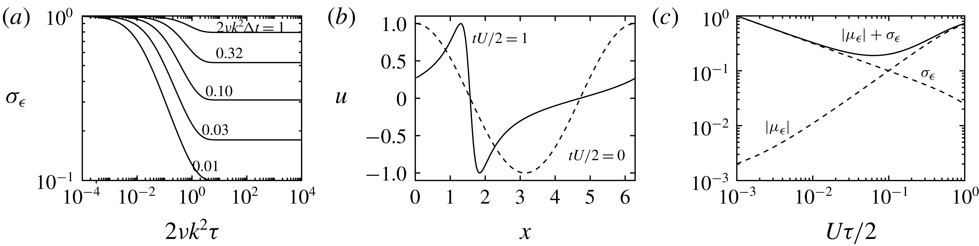
(a) Theoretical standard deviation of the reconstruction error $\unicode[STIX]{x1D70E}_{\unicode[STIX]{x1D716}}$  (3.17) for a diffusing Fourier mode, relative to the standard deviation of the measurement error of that mode $\unicode[STIX]{x1D70E}_{v}$ as a function of the dimensionless assimilation time $2\unicode[STIX]{x1D708}k^{2}\unicode[STIX]{x1D70F}$ for various dimensionless sampling times $2\unicode[STIX]{x1D708}k^{2}\unicode[STIX]{x0394}t$ . (b) The evolution of a scalar profile, with $u(t=0)=\cos (x)$ , that is advected by an inhomogeneous velocity field $U\cos (x)$ . (c) Theoretical standard deviation $\unicode[STIX]{x1D70E}_{\unicode[STIX]{x1D716}}$ and absolute value of mean $|\unicode[STIX]{x1D707}_{\unicode[STIX]{x1D716}}|$ of the reconstruction error (3.13) for the $k=1$ mode in non-uniform advection (3.18) based on a measurement filter, that only passes the $k=1$ mode (3.7).

Equation (3.17) is plotted in figure 1(a) as a function of $\unicode[STIX]{x1D70F}^{\prime }$ for various $\unicode[STIX]{x0394}t^{\prime }$ showing the transition from inverse square root to constant. The graph illustrates that the reconstruction does not improve when information is added beyond the correlation time of the system $\mathscr{T}=(2k^{2}\unicode[STIX]{x1D708})^{-1}$ , i.e. measurements at time $t_{i}\gg \mathscr{T}$ do not influence the reconstruction at time $t=0$ .

3.3 Advection

Next we consider the advection of a scalar $u$ in an inhomogeneous velocity field $U\cos (x)$ , with an amplitude $U$ and a unit wavenumber on a domain of size $2\unicode[STIX]{x03C0}$ . The evolution of a scalar profile $u(x,t)$ with $u(x,t=0)=\cos (x)$ is sketched in figure 1(b). The Fourier representation of the corresponding operator $S(u)=-U\cos (x)\unicode[STIX]{x2202}_{x}u$ is given by

(3.18) $$\begin{eqnarray}\displaystyle M^{kl}=-\frac{\unicode[STIX]{x1D55A}lU}{2}(\unicode[STIX]{x1D6FF}^{l,k-1}+\unicode[STIX]{x1D6FF}^{l,k+1}). & & \displaystyle\end{eqnarray}$$

We compute the error (3.13) in the small time limit $\unicode[STIX]{x1D70F}\Vert \boldsymbol{M}\Vert \ll 1$ , such that $\boldsymbol{G}_{i}$  (3.8b ) is approximated by

(3.19) $$\begin{eqnarray}\displaystyle \boldsymbol{G}_{i}\approx \unicode[STIX]{x1D739}+i\unicode[STIX]{x0394}t\boldsymbol{M}, & & \displaystyle\end{eqnarray}$$

which to leading order in $\unicode[STIX]{x1D70F}\Vert \boldsymbol{M}\Vert$ gives

(3.20) $$\begin{eqnarray}\displaystyle \boldsymbol{u}_{1}-\boldsymbol{v}_{1}=\left[\boldsymbol{F}-\unicode[STIX]{x1D739}+\frac{\unicode[STIX]{x1D70F}}{2}(\boldsymbol{F}\boldsymbol{\cdot }\boldsymbol{M}-\boldsymbol{M}\boldsymbol{\cdot }\boldsymbol{F})\right]\boldsymbol{\cdot }\boldsymbol{v}_{1}+P^{-1}\mathop{\sum }_{i=1}^{P}\boldsymbol{F}\boldsymbol{\cdot }\boldsymbol{v}_{i}^{\prime }, & & \displaystyle\end{eqnarray}$$

where we have used that $\unicode[STIX]{x1D70F}=\unicode[STIX]{x0394}tP$ . Using (3.7), (3.18), we see that the noise error (second term on the right-hand side of (3.20)) equals

(3.21) $$\begin{eqnarray}\displaystyle P^{-1}\mathop{\sum }_{i=1}^{P}F^{kl}v_{i}^{\prime l}=\left\{\begin{array}{@{}ll@{}}P^{-1}\displaystyle \mathop{\sum }_{i=1}^{P}v_{i}^{\prime k}, & \text{if }k\leqslant k_{filter},\\ 0, & \text{if }k>k_{filter},\end{array}\right. & & \displaystyle\end{eqnarray}$$

and the leading order of the filter error (first term on the right-hand side of (3.20)) equals

(3.22) $$\begin{eqnarray}\displaystyle \left[F^{kl}-\unicode[STIX]{x1D6FF}^{kl}+\frac{\unicode[STIX]{x1D70F}}{2}(F^{km}M^{ml}-M^{km}F^{ml})\right]v_{1}^{l}=\left\{\begin{array}{@{}ll@{}}0, & \text{if }k<k_{filter},\\ -\displaystyle \frac{1}{4}\unicode[STIX]{x1D55A}U\unicode[STIX]{x1D70F}(k+1)v^{k+1}, & \text{if }k=k_{filter},\\ v_{1}^{k}, & \text{if }k>k_{filter}.\end{array}\right. & & \displaystyle\end{eqnarray}$$

Equation (3.22) shows a 0 % and a 100 % error for $k<k_{filter}$ and $k>k_{filter}$ , and an intermediate error for $k=k_{filter}$ , which is explained as follows. When acting on the $k_{filter}$ mode at $t=0$ , the advection operator (3.18) creates $k_{filter}+1$ and $k_{filter}-1$ modes at $t=\unicode[STIX]{x1D70F}$ . Since the $k_{filter}+1$ mode is cut off by the filter (3.7), the resulting filtered signal at $t=\unicode[STIX]{x1D70F}$ contains insufficient information, to fully reconstruct the $k_{filter}$ mode at $t=0$ , which explains the intermediate filter error for $k=k_{filter}$ in (3.22). Combining (3.21), (3.22), we write for the total reconstruction error $\unicode[STIX]{x1D716}=u_{1}^{k_{filter}}-v_{1}^{k_{filter}}$ for the $k=k_{filter}$ mode

(3.23) $$\begin{eqnarray}\displaystyle u_{1}^{k_{filter}}-v_{1}^{k_{filter}}=-\frac{\unicode[STIX]{x1D55A}U\unicode[STIX]{x1D70F}(k_{filter}+1)}{4}v_{1}^{k_{filter}+1}+P^{-1}\mathop{\sum }_{i=1}^{P}v_{i}^{\prime k_{filter}}. & & \displaystyle\end{eqnarray}$$

The mean of the error $\unicode[STIX]{x1D707}_{\unicode[STIX]{x1D716}}$ is due to the filtering

(3.24a ) $$\begin{eqnarray}\displaystyle \unicode[STIX]{x1D707}_{\unicode[STIX]{x1D716}}=-\frac{\unicode[STIX]{x1D55A}U\unicode[STIX]{x1D70F}(k_{filter}+1)}{4}v_{1}^{k_{filter}+1}, & & \displaystyle\end{eqnarray}$$

and the standard deviation of the error $\unicode[STIX]{x1D70E}_{\unicode[STIX]{x1D716}}$ is due to the noise

(3.24b ) $$\begin{eqnarray}\displaystyle \unicode[STIX]{x1D70E}_{\unicode[STIX]{x1D716}}=\unicode[STIX]{x1D70E}_{v}\sqrt{\frac{\unicode[STIX]{x0394}t}{\unicode[STIX]{x1D70F}}}, & & \displaystyle\end{eqnarray}$$

where we have used that $P=\unicode[STIX]{x1D70F}/\unicode[STIX]{x0394}t$ , and that $v_{i}^{\prime k_{filter}}$ are uncorrelated random variables with a standard deviation $\unicode[STIX]{x1D70E}_{v}$ . The (absolute value of the) filter error (3.24a ) increases with the assimilation time $\unicode[STIX]{x1D70F}$ , since the advection operator (3.18) re-distributes the Fourier modes from the resolved part of the spectrum $k\leqslant k_{filter}$ to the unresolved part $k>k_{filter}$ . The noise error (3.24b ), on the other hand, decreases with $\unicode[STIX]{x1D70F}$ , i.e. it decreases as the inverse square root of the number of samples $P\sim \unicode[STIX]{x1D70F}$ , similar as in the diffusion problem (3.17).

It is recalled, that $\unicode[STIX]{x1D707}_{\unicode[STIX]{x1D716}}$ and $\unicode[STIX]{x1D70E}_{\unicode[STIX]{x1D716}}$ in (3.24) are obtained by linearly expanding $\boldsymbol{G}_{i}$ in $i\unicode[STIX]{x0394}t$  (3.19). In figure 1(c) we plot $\unicode[STIX]{x1D707}_{\unicode[STIX]{x1D716}}$ and $\unicode[STIX]{x1D70E}_{\unicode[STIX]{x1D716}}$ , based on the full nonlinear operator (3.8b ), and by numerically evaluating (3.7), (3.13), (3.18), where we have used $k_{filter}=1$ . In agreement with (3.24), the figure shows that the (absolute value of the) filter error $|\unicode[STIX]{x1D707}_{\unicode[STIX]{x1D716}}|$ increases, and the noise error $\unicode[STIX]{x1D70E}_{\unicode[STIX]{x1D716}}$ decreases, both as functions of  $\unicode[STIX]{x1D70F}$ .

4.1 Set-up

In this section we study the performance of the STIM (2.2), to improve the accuracy of synthetic PIV data for a 2-D incompressible, decaying turbulent velocity field $\boldsymbol{v}$ , on a square bi-periodic domain of size $L=2\unicode[STIX]{x03C0}$ . The flow starts at $t=0$ from a random velocity field, with a velocity norm of $\mathscr{U}=\Vert \boldsymbol{v}\Vert =1$ .

It is emphasised, that the present test case is a purely 2-D flow, which may be realised in the laboratory using large aspect ratio flow cells (e.g. Shats et al. Reference Shats, Xia, Punzmann and Falkovich2007) or soap films (e.g. Gillissen et al. Reference Gillissen, Vilquin, Kellay, Bouffanais and Yue2018). Since the reconstruction principles are equivalent in two and three dimensions, these principles are studied most effectively in two dimensions. Purely 2-D flow is not to be confused with planar PIV measurements of a 3-D flow. In this context, it is noted, that measuring turbulence in a single plane is insufficient to reconstruct volumetric turbulence, which instead requires three-dimensional PIV, involving for instance the use of four cameras, and tomographic reconstruction algorithms (e.g. Scarano Reference Scarano2012). It is further noted that the characteristics of the measurement errors in tomographic PIV are different than in standard PIV, and the ability of STIM to reduce these errors deserves further study.

We non-dimensionalise our variables using the velocity scale $\mathscr{U}$ , and the length scale $L/(2\unicode[STIX]{x03C0})$ , which corresponds to a time scale $L/(2\unicode[STIX]{x03C0}\mathscr{U})$ . Starting from random conditions at $t=0$ , the flow takes a few time units to develop physical structures. We apply the reconstruction thereafter, i.e. within the period $2<t<2+T$ , where the reconstruction interval is chosen to be $T=10$ . We define the following PIV errors for the kinetic energy $\tilde{\unicode[STIX]{x1D716}}_{K}$ :

(4.1) $$\begin{eqnarray}\displaystyle \tilde{\unicode[STIX]{x1D716}}_{K}=T^{-1}\int _{2}^{2+T}\frac{\displaystyle \int (\tilde{\boldsymbol{v}}-\boldsymbol{v})^{2}\,\text{d}V}{\displaystyle \int \boldsymbol{v}^{2}\,\text{d}V}\,\text{d}t, & & \displaystyle\end{eqnarray}$$

for the pressure $\tilde{\unicode[STIX]{x1D716}}_{p}$

(4.2) $$\begin{eqnarray}\displaystyle \tilde{\unicode[STIX]{x1D716}}_{p}=T^{-1}\int _{2}^{2+T}\frac{\displaystyle \int p^{2}(\tilde{\boldsymbol{v}}-\boldsymbol{v})\,\text{d}V}{\displaystyle \int p^{2}(\boldsymbol{v})\,\text{d}V}\,\text{d}t, & & \displaystyle\end{eqnarray}$$

and for the energy dissipation $\tilde{\unicode[STIX]{x1D716}}_{\mathscr{D}}$

(4.3) $$\begin{eqnarray}\displaystyle \tilde{\unicode[STIX]{x1D716}}_{\mathscr{D}}=T^{-1}\int _{2}^{2+T}\frac{\displaystyle \int \mathscr{D}(\tilde{\boldsymbol{v}}-\boldsymbol{v})\,\text{d}V}{\displaystyle \int \mathscr{D}(\boldsymbol{v})\,\text{d}V}\,\text{d}t, & & \displaystyle\end{eqnarray}$$

where it is recalled that $\boldsymbol{v}$ is the true velocity field and $\tilde{\boldsymbol{v}}$ is the synthetic PIV velocity field. The dissipation field is given by

(4.4) $$\begin{eqnarray}\displaystyle \mathscr{D}(\boldsymbol{u})=\unicode[STIX]{x1D708}\unicode[STIX]{x1D735}\boldsymbol{u}\boldsymbol{ : }\unicode[STIX]{x1D735}\boldsymbol{u}, & & \displaystyle\end{eqnarray}$$

and the pressure field is computed from the equation of state

(4.5) $$\begin{eqnarray}\displaystyle \unicode[STIX]{x1D6FB}^{2}p(\boldsymbol{u})=-\unicode[STIX]{x1D735}\unicode[STIX]{x1D735}\boldsymbol{ : }\boldsymbol{u}\boldsymbol{u}, & & \displaystyle\end{eqnarray}$$

and reads in Fourier space

(4.6) $$\begin{eqnarray}\displaystyle p^{\boldsymbol{k}}(\boldsymbol{u})=-\frac{\boldsymbol{k}\boldsymbol{k}\mathbf{:}\boldsymbol{u}^{\boldsymbol{k}}\boldsymbol{u}^{\boldsymbol{k}}}{k^{2}}, & & \displaystyle\end{eqnarray}$$

where the superscript indices refer to the Fourier wavevectors. Similarly we define the following reconstruction errors for the kinetic energy $\unicode[STIX]{x1D716}_{K}$

(4.7) $$\begin{eqnarray}\displaystyle \unicode[STIX]{x1D716}_{K}=T^{-1}\int _{2}^{2+T}\frac{\displaystyle \int (\boldsymbol{u}-\boldsymbol{v})^{2}\,\text{d}V}{\displaystyle \int \boldsymbol{v}^{2}\,\text{d}V}\,\text{d}t, & & \displaystyle\end{eqnarray}$$

for the pressure $\unicode[STIX]{x1D716}_{p}$

(4.8) $$\begin{eqnarray}\displaystyle \unicode[STIX]{x1D716}_{p}=T^{-1}\int _{2}^{2+T}\frac{\displaystyle \int p^{2}(\boldsymbol{u}-\boldsymbol{v})\,\text{d}V}{\displaystyle \int p^{2}(\boldsymbol{v})\,\text{d}V}\,\text{d}t, & & \displaystyle\end{eqnarray}$$

and for the energy dissipation $\unicode[STIX]{x1D716}_{\mathscr{D}}$

(4.9) $$\begin{eqnarray}\displaystyle \unicode[STIX]{x1D716}_{\mathscr{D}}=T^{-1}\int _{2}^{2+T}\frac{\displaystyle \int \mathscr{D}(\boldsymbol{u}-\boldsymbol{v})\,\text{d}V}{\displaystyle \int \mathscr{D}(\boldsymbol{v})\,\text{d}V}\,\text{d}t, & & \displaystyle\end{eqnarray}$$

where it is recalled that $\boldsymbol{u}$ is the reconstructed velocity field.

The reconstruction time interval $2<t<2+T$ is split into segments of size $\unicode[STIX]{x1D70F}$ , referred to as the assimilation time. In each of these segments, a reconstruction problem is solved, which finds the velocity field at the start of that segment $\boldsymbol{u}_{1}$ . While the initial guess for the initial conditions of the first segment is zero: $\boldsymbol{u}_{1}=\mathbf{0}$ , a considerable improvement of the reconstruction is achieved by using for the initial guess for the initial conditions of the following segments, the final conditions of each previous segment (Gillissen et al. 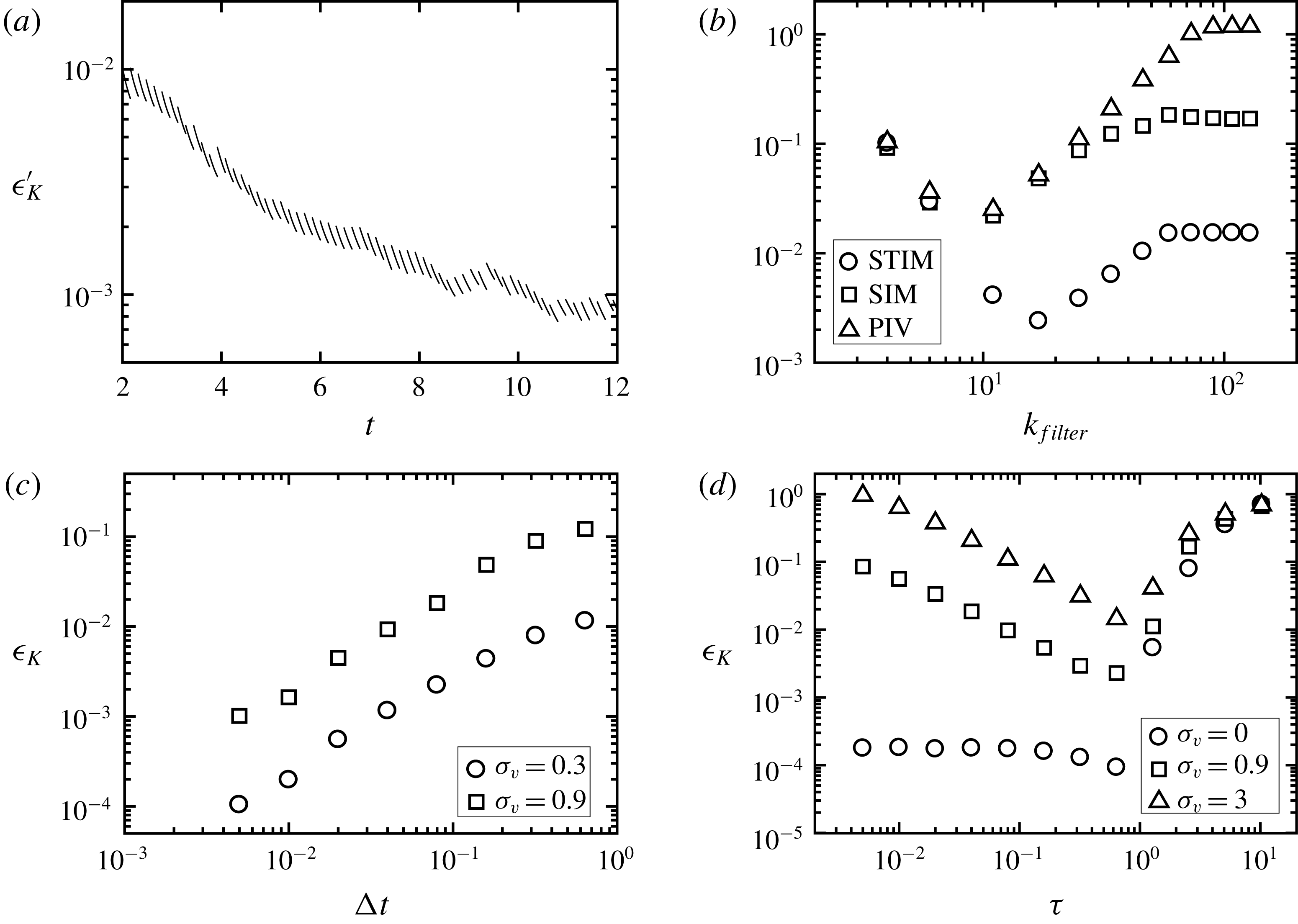Reference Gillissen, Vilquin, Kellay, Bouffanais and Yue2018). Figure 3(a) illustrates this improvement, by plotting the time dependence of the instantaneous reconstruction error in the kinetic energy $\unicode[STIX]{x1D716}_{K}^{\prime }$

(4.10) $$\begin{eqnarray}\displaystyle \unicode[STIX]{x1D716}_{K}^{\prime }=\frac{\displaystyle \int (\boldsymbol{u}-\boldsymbol{v})^{2}\,\text{d}V}{\displaystyle \int \boldsymbol{v}^{2}\,\text{d}V}. & & \displaystyle\end{eqnarray}$$

In this figure each line segment corresponds to one assimilation window with a time interval of $\unicode[STIX]{x1D70F}$ .

The synthetic PIV data $\tilde{\boldsymbol{v}}$ are generated by adding noise to the true velocity field  $\boldsymbol{v}$ . The true velocity field is generated by numerically simulating the Navier–Stokes equations (2.1), which in the absence of forcing mechanisms, and starting from random initial conditions, results in freely decaying turbulence. The numerical method uses Fourier functions to compute spatial derivatives (e.g. Canuto et al. Reference Canuto, Hussaini, Quarteroni and Thomas1988). Time integration is performed using the second-order explicit Adams–Bashforth scheme for the advection terms and the second-order implicit Crank–Nicolson scheme for the diffusion terms. The number of grid points is $N^{2}=128^{2}$ , which is sufficient to resolve all length scales, and the numerical integration time step is $1\times 10^{-3}$ , which is sufficiently small, such that the numerical solution does not change upon reducing the time step. The initial random velocity field is constructed by assigning random numbers to the Fourier modes, whose absolute wavevectors $|\boldsymbol{k}|\leqslant 8$ , while the remaining Fourier modes are assumed zero. The initial velocity field is normalised, such that $\mathscr{U}=\Vert \boldsymbol{v}\Vert =1$ at $t=0$ . The viscosity is $\unicode[STIX]{x1D708}=7.3\times 10^{-4}$ , which corresponds to a Reynolds number, based on the velocity scale $\mathscr{U}=1$ and on the domain size $L=2\unicode[STIX]{x03C0}$ , of $Re=\mathscr{U}L/\unicode[STIX]{x1D708}=8.6\times 10^{3}$ . The correlation time of the resulting turbulent flow is around $\mathscr{T}\sim 1$ , see figure 2(a).

Figure 2.

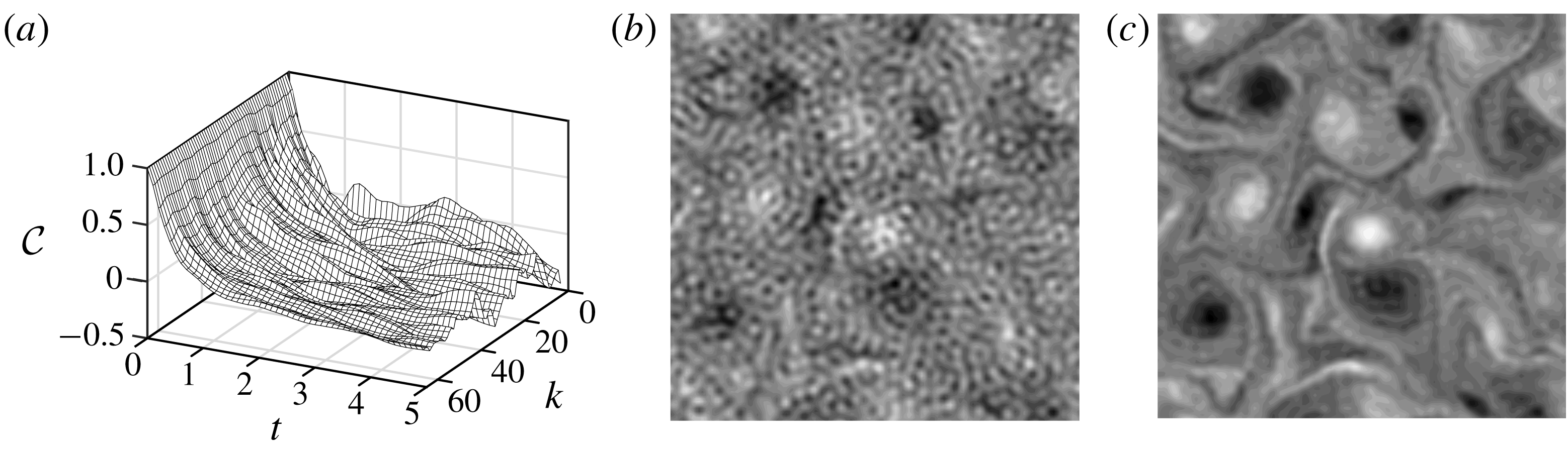
(a) Auto-correlation ${\mathcal{C}}$ of the various modes (with absolute wavevector $k$ ), of the true vorticity field $\unicode[STIX]{x1D735}\times \boldsymbol{v}$ , as a function of the time distance $t$ between the pair of values, obtained by analysing data in the time interval $2<t<12$ . (b) Vorticity field at time $t=2$ of the synthetic PIV data $\unicode[STIX]{x1D735}\times \tilde{\boldsymbol{v}}$ using a noise level of $\unicode[STIX]{x1D70E}_{v}=0.3$ , and a reciprocal filter width of $k_{filter}=32$ . (c) Vorticity field at time $t=2$ of the corresponding STIM reconstruction $\unicode[STIX]{x1D735}\times \boldsymbol{u}$ , using an assimilation time of $\unicode[STIX]{x1D70F}=0.16$ and a sampling time of $\unicode[STIX]{x0394}t=5\times 10^{-3}$ .

Figure 3.

STIM performance for idealised synthetic PIV data with white noise. (a) Instantaneous STIM reconstruction error in the kinetic energy $\unicode[STIX]{x1D716}_{K}^{\prime }$  (4.10) as a function of time $t$ , using a reciprocal filter width of $k_{filter}=16$ , a noise level of $\unicode[STIX]{x1D70E}_{v}=0.3$ , an assimilation time of $\unicode[STIX]{x1D70F}=0.16$ and a sampling time of $\unicode[STIX]{x0394}t=5\times 10^{-3}$ . (b) PIV error in the kinetic energy $\tilde{\unicode[STIX]{x1D716}}_{K}$  (4.1) (triangles) and reconstruction error in the kinetic energy $\unicode[STIX]{x1D716}_{K}$  (4.7) using STIM (circles) and SIM (squares), as functions of $k_{filter}$ , using $\unicode[STIX]{x1D70E}_{v}=0.9$ , $\unicode[STIX]{x1D70F}=0.16$ and $\unicode[STIX]{x0394}t=5\times 10^{-3}$ . (c) STIM reconstruction error $\unicode[STIX]{x1D716}_{K}$ as a function of $\unicode[STIX]{x0394}t$ , using $k_{filter}=32$ , $\unicode[STIX]{x1D70F}=0.64$ and varying $\unicode[STIX]{x1D70E}_{v}$ . (d) STIM reconstruction error $\unicode[STIX]{x1D716}_{K}$ as a function of $\unicode[STIX]{x1D70F}$ , using $k_{filter}=32$ , $\unicode[STIX]{x0394}t=5\times 10^{-3}$ and varying $\unicode[STIX]{x1D70E}_{v}$ . In (b–d), $\unicode[STIX]{x1D716}_{K}$ and $\tilde{\unicode[STIX]{x1D716}}_{K}$ are averaged over five reconstructions, using different true velocity fields $\boldsymbol{v}$ with different (random) initial conditions.

To generate synthetic PIV data $\tilde{\boldsymbol{v}}$ , we add noise to the simulated, true velocity field $\boldsymbol{v}$ . In this work we consider two types of noise. First, we consider in § 4.2 white PIV noise, which is an idealisation compared to realistic PIV noise. This simplification, however, allows for a systematic variation of the noise properties and a clear interpretation of the method performance, through a comparison with the analytical results in § 3. In addition, we consider in § 4.3, realistic PIV noise, that are generated by computationally mimicking the PIV measurement process. To this end we employ a simplistic PIV algorithm, without employing state of the art PIV noise reduction techniques. The resulting synthetic PIV error is highly correlated, which provides an extremely stringent test case for STIM. This is opposite to the white noise error in § 4.2, which is tackled effectively by STIM. The extreme cases of white noise and simplistic PIV noise mark the upper and lower boundaries for the effectiveness of the STIM.

4.2 White PIV noise

First we consider idealised PIV data $\tilde{\boldsymbol{v}}$ , which are constructed by adding white noise to the true velocity field $\boldsymbol{v}$ , and subsequently applying a filter (3.5). The standard deviation of the noise $\unicode[STIX]{x1D70E}_{v}$ is referred to as the noise level, and the reciprocal filter width is denoted $k_{filter}=2\unicode[STIX]{x03C0}/\ell$ .

Figure 2(b) visualises the resulting synthetic PIV vorticity field $\unicode[STIX]{x1D735}\times \tilde{\boldsymbol{v}}$ at $t=2$ , using a noise level of $\unicode[STIX]{x1D70E}_{v}=0.3$ and a reciprocal filter width of $k_{filter}=32$ . The corresponding reconstructed vorticity $\unicode[STIX]{x1D735}\times \boldsymbol{u}$ , that is produced by the STIM, is shown in figure 2(c), where we have used an assimilation time of $\unicode[STIX]{x1D70F}=0.16$ and a sampling time of $\unicode[STIX]{x0394}t=5\times 10^{-3}$ . The noise in the reconstruction is significantly reduced, as compared to the synthetic PIV data in figure 2(b).

Figure 3(b) shows the PIV error in the kinetic energy $\tilde{\unicode[STIX]{x1D716}}_{K}$  (4.1) as a function of the reciprocal filter width $k_{filter}$ for a noise level of $\unicode[STIX]{x1D70E}_{v}=0.9$ . It is seen that $\tilde{\unicode[STIX]{x1D716}}_{K}$ depends non-monotonically on $k_{filter}$ , i.e. an initial decrease is followed by an increase. This non-monotonicity reflects, that low wavenumber modes contain more flow structure than noise, while large wavenumber modes contain more noise than structure. Low wavenumber modes therefore improve the measurement, while high wavenumber modes deteriorate the measurement.

Figure 3(b) also shows the corresponding STIM reconstruction error in the kinetic energy $\unicode[STIX]{x1D716}_{K}$  (4.7) as a function of $k_{filter}$ , where we have used an assimilation time of $\unicode[STIX]{x1D70F}=0.16$ and a sampling time of $\unicode[STIX]{x0394}t=5\times 10^{-3}$ . It is seen that $\unicode[STIX]{x1D716}_{K}$ follows the non-monotonic trend of the PIV error $\tilde{\unicode[STIX]{x1D716}}_{K}$ . For $k_{filter}\leqslant 4$ , the STIM does not improve the PIV data, i.e. $\tilde{\unicode[STIX]{x1D716}}_{K}\approx \unicode[STIX]{x1D716}_{K}$ , while for $k_{filter}\geqslant 4$ , the STIM improves the accuracy of the data, with a maximum error reduction of two decades in the absence of spatial filtering, i.e. for $k_{filter}=N=128$ .

Next we compare the performance of the STIM (2.2) to that of the SIM (2.9). Whereas STIM reduces measurement noise by fitting a solution to the Navier–Stokes equation to time-dependent measurement data, SIM achieves this, by applying a hyper diffusion process to the measurement data. The hyper diffusivity is referred to as the regularisation strength $\unicode[STIX]{x1D705}$ . This parameter must be chosen sufficiently large, as to dampen the small-scale noise, and sufficiently small, as to not affect the large-scale, energy-containing eddies. A parametric study (not shown) revealed that $\unicode[STIX]{x1D705}=10^{-6}$ $\mathscr{U}[L/(2\unicode[STIX]{x03C0})]^{3}$ is a suitable value, for the test case at hand. Figure 3(b) shows the resulting SIM reconstruction error in the kinetic energy $\unicode[STIX]{x1D716}_{K}$  (4.7) as a function of $k_{filter}$ . As expected, SIM is less effective in reducing the measurement error than STIM. In the absence of spatial filtering ( $k_{filter}=N=128$ ) SIM achieves a tenfold reduction in measurement error, whereas STIM achieves a hundredfold reduction under identical conditions.

As STIM fits a solution to the Navier–Stokes equation to time-dependent measurement data, the performance of STIM, in the case of white measurement noise, increases with the sampling frequency, i.e. the STIM reconstruction error $\unicode[STIX]{x1D716}_{K}$  (4.7) increases with the sampling time $\unicode[STIX]{x0394}t$ . This feature is illustrated in figure 3(c), where we plot $\unicode[STIX]{x1D716}_{K}$ as a function of $\unicode[STIX]{x0394}t$ , and where we have used a reciprocal filter width of $k_{filter}=32$ , an assimilation time of $\unicode[STIX]{x1D70F}=0.64$ and various noise levels $\unicode[STIX]{x1D70E}_{v}$ . The data in figure 3(c) show that the error in the kinetic energy $\unicode[STIX]{x1D716}_{K}$ depends linearly on $\unicode[STIX]{x0394}t$ which is consistent with the square root dependence of the scalar error on $\unicode[STIX]{x0394}t$ for the linear diffusion problem (3.17).

Figure 3(d) shows the STIM reconstruction error $\unicode[STIX]{x1D716}_{K}$  (4.7) as a function of the assimilation time $\unicode[STIX]{x1D70F}$ for a reciprocal filter width $k_{filter}=32$ , a sampling time of $\unicode[STIX]{x0394}t=5\times 10^{-3}$ and for various noise levels $\unicode[STIX]{x1D70E}_{v}$ . It is seen that $\unicode[STIX]{x1D716}_{K}$ depends non-monotonically on $\unicode[STIX]{x1D70F}$ , where for small $\unicode[STIX]{x1D70F}$ the error decreases, while for large $\unicode[STIX]{x1D70F}$ the error increases, in qualitative agreement with linear theory (3.17), (3.24). This error increase reflects that information de-correlates over long times, making the inverse problem of minimising (2.2) ill-posed. In the linear advection problem, a similar increase in the reconstruction error $\unicode[STIX]{x1D716}_{K}$ with $\unicode[STIX]{x1D70F}$ was observed ((3.24b ); figure 1 c), which is related to the loss of information from the resolved modes into the unresolved (filtered) modes. This loss of information therefore bears an analogy with the de-correlation of information in the 2-D turbulent flow, which corresponds to a dissipation of kinetic energy, via the energy cascade, into heat.

4.3 Realistic PIV noise

Next we generate synthetic velocimetry data with realistic PIV noise by computing trajectories of passive point particles. The total number of particles $N_{p}(L/\ell )^{2}$ is chosen such, that there are on average $N_{p}$ particles inside the PIV interrogation window of size $\ell$ . The interrogation window corresponds to $32^{2}$ image pixels. The image size of the total domain is therefore $(32L/\ell )^{2}$ pixels. Each particle generates a light intensity image, which is a Gaussian function with a standard deviation of 0.7 pixels. A PIV image is constructed by superimposing the Gaussian images of all the particles. To compute the PIV velocity field at $t=t_{i}$ , we generate two particle images at $t=t_{i}-{\textstyle \frac{1}{2}}\unicode[STIX]{x0394}t_{PIV}$ and $t=t_{i}+{\textstyle \frac{1}{2}}\unicode[STIX]{x0394}t_{PIV}$ . The image time difference equals $\unicode[STIX]{x0394}t_{PIV}=0.02\ell /\mathscr{U}$ . To find the PIV velocity vector at position $\boldsymbol{x}$ we apply a mask of width $\ell$ and centre $\boldsymbol{x}$ to these images, and maximise the correlation between the masked images at $t=t_{i}-{\textstyle \frac{1}{2}}\unicode[STIX]{x0394}t_{PIV}$ and $t=t_{i}+{\textstyle \frac{1}{2}}\unicode[STIX]{x0394}t_{PIV}$ , as given in (1.1). The PIV velocity field is determined using a sliding interrogation window on $N^{2}=128^{2}$ spatial points, which is the same spatial grid, as is used in the fluid flow simulations. The location of the correlation maximum is determined with sub-pixel accuracy by fitting a paraboloid to the correlation function in a region of $3\times 3$ pixels around the pixel with the largest intensity.

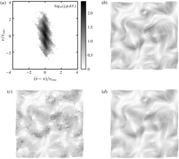
We apply the PIV algorithm described above, to the simulated two-dimensional turbulent flow, which is described in § 4.1. The resulting synthetic PIV error $\tilde{\boldsymbol{v}}-\boldsymbol{v}$ is correlated with the true velocity $\boldsymbol{v}$ , as shown by the joint probability density function of $\tilde{\boldsymbol{v}}-\boldsymbol{v}$ and $\boldsymbol{v}$ in figure 4(a). Figures 4(b), 4(c) and 4(d) compare the corresponding true velocity field $\boldsymbol{v}$ the synthetic PIV velocity field $\tilde{\boldsymbol{v}}$ and the reconstructed velocity field $\boldsymbol{u}$ using STIM, respectively. The comparison shows, that STIM significantly improves the accuracy of the PIV data. The data in figure 4 are taken at time $t=4$ , using a reciprocal filter width of $k_{filter}=2\unicode[STIX]{x03C0}/\ell =32$ , a PIV particle density of $N_{p}=2$ , an assimilation time of $\unicode[STIX]{x1D70F}=0.64$ and a sampling time of $\unicode[STIX]{x0394}t=5\times 10^{-3}$ .

Figure 4.

(a) Joint probability density function (j.p.d.f.) of $\tilde{\boldsymbol{v}}-\boldsymbol{v}$ and $\boldsymbol{v}$ , where $\tilde{\boldsymbol{v}}$ is the synthetic PIV velocity field and $\boldsymbol{v}$ is the true velocity field. (b) Snapshot of the true velocity field $\boldsymbol{v}$ . (c) Snapshot of the synthetic PIV velocity field $\tilde{\boldsymbol{v}}$ . (d) Snapshot of the STIM reconstructed velocity field $\boldsymbol{u}$ . The data in (a–d) are taken at time $t=4$ , using a reciprocal filter width of $k_{filter}=2\unicode[STIX]{x03C0}/\ell =32$ , an assimilation window of $\unicode[STIX]{x1D70F}=0.64$ and a sampling time of $\unicode[STIX]{x0394}t=5\times 10^{-3}$ .

Figure 5.

STIM performance for synthetic velocimetry data with realistic PIV noise. (a) The PIV error in the kinetic energy $\tilde{\unicode[STIX]{x1D716}}_{K}$  (4.1) as a function of the PIV particle density $N_{p}$ , using a reciprocal filter width of $k_{filter}=2\unicode[STIX]{x03C0}/\ell =32$ , an assimilation time of $\unicode[STIX]{x1D70F}=0.64$ and a sampling time of $\unicode[STIX]{x0394}t=5\times 10^{-3}$ . (b) The PIV error in the kinetic energy $\tilde{\unicode[STIX]{x1D716}}_{K}$ (grey circles; (4.1)), in the pressure $\tilde{\unicode[STIX]{x1D716}}_{p}$ (grey squares; (4.2)) and in the energy dissipation $\tilde{\unicode[STIX]{x1D716}}_{\mathscr{D}}$ (grey triangles; (4.3)) and the STIM reconstruction error in the kinetic energy $\unicode[STIX]{x1D716}_{K}$ (white circles; (4.7)), in the pressure $\unicode[STIX]{x1D716}_{p}$ (white squares; (4.8)) and in the energy dissipation $\unicode[STIX]{x1D716}_{\mathscr{D}}$ (white triangles; (4.9)) as functions of $k_{filter}$ , using $N_{p}=2$ , $\unicode[STIX]{x1D70F}=0.64$ and $\unicode[STIX]{x0394}t=5\times 10^{-3}$ . (c) The STIM reconstruction error in the kinetic energy $\unicode[STIX]{x1D716}_{K}$ (4.7) as a function of $\unicode[STIX]{x0394}t$ , using $k_{filter}=32$ , $N_{p}=2$ and $\unicode[STIX]{x1D70F}=\unicode[STIX]{x0394}t$ . In (a–c), the presented errors are averaged over five simulations, using different true velocity fields $\boldsymbol{v}$ with different (random) initial conditions.

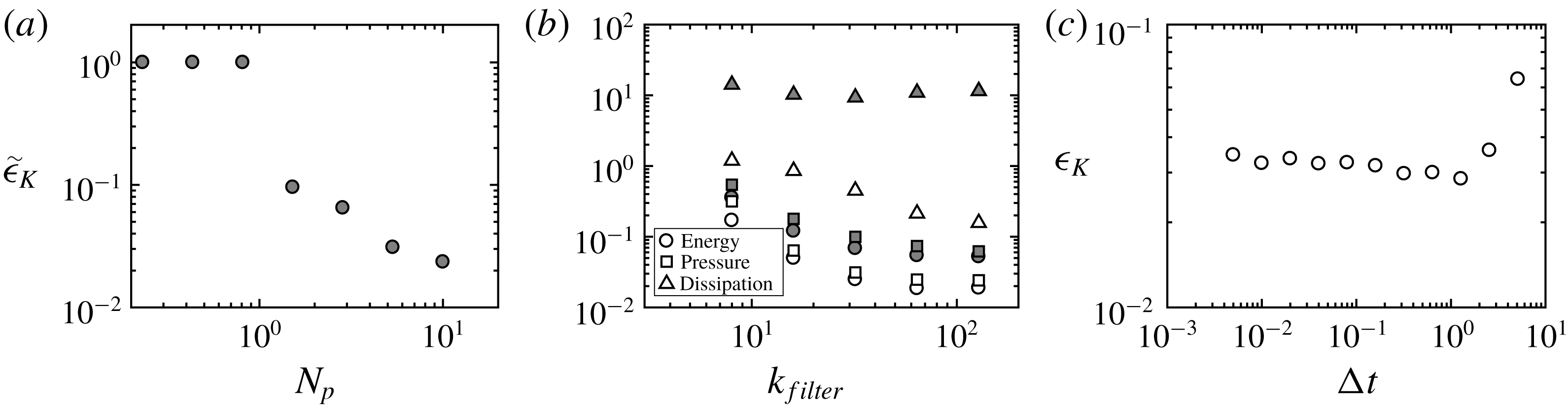
In figure 5(a), we study the PIV error in the kinetic energy $\tilde{\unicode[STIX]{x1D716}}_{K}$ (4.1) as a function of $N_{p}$ , using $k_{filter}=32$ , $\unicode[STIX]{x1D70F}=0.64$ and $\unicode[STIX]{x0394}t=5\times 10^{-3}$ . As expected $N_{p}<1$ is ineffective, resulting in a 100 % error $\tilde{\unicode[STIX]{x1D716}}_{K}\approx 1$ . When $N_{p}$ exceeds unity, $\tilde{\unicode[STIX]{x1D716}}_{K}$ drops sharply, and for large $N_{P}$ the error saturates at $\tilde{\unicode[STIX]{x1D716}}_{K}\sim 10^{-2}$ .

In figure 5(b) we study the PIV error in the kinetic energy $\tilde{\unicode[STIX]{x1D716}}_{K}$ (4.1) in the pressure $\tilde{\unicode[STIX]{x1D716}}_{p}$ (4.2) and in the energy dissipation $\tilde{\unicode[STIX]{x1D716}}_{\mathscr{D}}$ (4.3) as functions of $k_{filter}$ , using $N_{p}=2$ . The PIV error in the pressure $\tilde{\unicode[STIX]{x1D716}}_{p}$ is similar to that in the kinetic energy $\tilde{\unicode[STIX]{x1D716}}_{K}$ , and these errors increase with decreasing $k_{filter}$ . This reflects, that a larger interrogation window $\ell$ cuts off more energy, resulting in larger errors. The PIV error for the dissipation $\tilde{\unicode[STIX]{x1D716}}_{\mathscr{D}}$ is two orders of magnitude larger than that for the energy and the pressure, and $\tilde{\unicode[STIX]{x1D716}}_{\mathscr{D}}$ is independent of $k_{filter}$ . This independence reflects, that the dissipative scales are poorly captured by the PIV image correlation algorithm, irrespective of $k_{filter}$ , in the range considered.

In addition to the PIV errors, we also plot in figure 5(b), the corresponding STIM reconstruction errors for the kinetic energy $\unicode[STIX]{x1D716}_{K}$ (4.7), the pressure $\unicode[STIX]{x1D716}_{p}$  (4.8) and the dissipation $\unicode[STIX]{x1D716}_{\mathscr{D}}$  (4.9), where we used $\unicode[STIX]{x1D70F}=0.64$ and $\unicode[STIX]{x0394}t=5\times 10^{-3}$ . It is seen, that STIM reduces the PIV error by a factor of around three for both the energy and the pressure, while it reduces the error for the dissipation by a factor of up to 100. This result illustrates, that STIM significantly improves the structure of the dissipating eddies, which are generally poorly represented by PIV. This conclusion is also supported by the snapshots in figure 4.

STIM (2.2) fits a solution of the Navier–Stokes equations to time-dependent measurement data. We have seen in figure 3(d), that, in the case of white measurement noise, the accuracy of the fit can be made arbitrarily small, by increasing the data density, i.e. by reducing the sampling time $\unicode[STIX]{x0394}t$ . For realistic PIV noise, the situation is different, however. This is illustrated in figure 5(c), showing, that for synthetic velocimetry data with realistic PIV noise, the STIM reconstruction error in the kinetic energy $\unicode[STIX]{x1D716}_{K}$ does not depend on $\unicode[STIX]{x0394}t$ , provided that $\unicode[STIX]{x0394}t$ is smaller than the flow correlation time $\mathscr{T}\sim 1$ (figure 2 a). This means, that the maximum sampling time, that still produces a reasonable reconstruction, is of the order of the flow correlation time, and adding more intermediate samples does not necessarily improve the reconstruction.