I. INTRODUCTION AND BACKGROUND
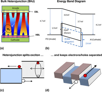
A bulk-heterojunction organic photovoltaic (BHJ-OPV) solar cellReference Yu, Gao, Hummelen, Wudl and Heeger1–Reference Nelson5 consists of two demixed, phase-segregated, bicontinuous, donor–acceptor organic semiconductors capped by a transparent anode and a metallic cathode, see Fig. 1. Although a wide variety of organic semiconductorsReference Nelson5–Reference Park, Roy, Beaupre, Cho, Coates, Moon, Moses, Leclerc, Lee and Heeger7 have been analyzed, we will consider hole-conducting P3HT and electron-conducting PCBM [red and blue regions in Fig. 1(a)] as an illustrative exampleReference Shaheen, Brabec, Sariciftci, Padinger, Fromherz and Hummelen8–Reference Ma, Yang, Gong, Lee and Heeger11 and explore how the fundamental physical properties of polymers translate to ultimate panel efficiency reported in the literature. The operation of BHJ-OPV is often explained as followsReference Blom, Mihailetchi, Koster and Markov12–Reference Kirchartz, Taretto and Rau15: excitons generated by sunlight in such organic semiconductor composite are localized in single conjugated unit of few nanometers and held together by undiluted Coulomb attraction between the charges, typical of low dielectric constant materials. Therefore, if the excitons are not dissociated into free electrons and holes by atomically sharp quasielectric field of donor/acceptor interface [see Figs. 1(b)–1(d)], they would be lost due to self-recombination. If the phase-segregated morphology is viewed as entangled (or intercalatedReference Mayer, Toney, Scully, Rivnay, Brabec, Scharber, Koppe, Heeney, McCulloch and McGehee16) regions of donor-rich and acceptor-rich organic semiconductors, as in Fig. 1(a), one finds that the effective cross-sectional “diameter” of each phase evolves continuously with anneal time, i.e., W D(t a). During the initial transient of phase separation, the donor/acceptor (D/A) interface is diffuse, and the quasifield may not be strong enough for exciton dissociation. However, the annealing conditions need to be precisely controlled for fabricating the efficient morphology,Reference Ray, Nair and Alam17 which should have the following properties: both the D–A phases form percolating pathways to the electrodes, the average D/A domain size (W D) is comparable to the exciton diffusion length,  $L_{{\rm{ex}}} \, = \,\sqrt {D{\rm{\tau }}_{{\rm{ex}}} } $, and the D/A interface is sharply defined, so that the excitons can reach and be dissociated by the heterojunction with high efficiency, see Fig. 1(c). Once dissociated, electrons and holes are spatially separated in their respective polymer channels and remain isolated from each other by the D–A heterojunction (which is typically a type II heterobarrierReference Sze18) with staggered band gaps, as shown in Fig. 1(d). The lack of minority carriers in the electron-transporting and hole-transporting regions suppresses bulk recombination, and the high internal field created by the electrode work–function difference [Fig. 1(b)] sweeps the free carriers out before they can recombine at the interface. This efficient exciton dissociation, spatial free carrier isolation, and drift-dominated transport of photogenerated carriers explain the exceptionally high quantum efficiency of a BHJ-OPV.
(a) The red and blue regions define the donor and the acceptor materials of a BHJ-OPV, respectively. EBL: electron-blocking layer; HBL: hole-blocking layer. (b–d) The band diagrams of BHJ-OPV from various perspectives. (b) The band diagrams along the lines (1) and (2) indicated in (a). The built-in field and the staggered type II discontinuity of the P3HT/PCBM band alignment are clearly shown. (c) When excitons are generated in one of the materials, they must find a donor/acceptor heterointerface for effective charge separation. (d) Once separated, the type II potential confines electrons and holes in their respective channels, so that recombination occurs only at the D/A interface.

Does improvement in J SC guarantees high efficiency of an organic solar cell?Reference Kirchartz, Taretto and Rau15, Reference Giebink, Wiederrecht, Wasielewski and Forrest19–Reference Servaites, Ratner and Marks21 Not necessarily! Since η = J SC × V OC × FF, overall efficiency can only improve if both the open-circuit voltage (V OC) and the fill factor (FF) improve with morphology and device parameters. A key concern is that a large D/A interfacial area (A itf) not only increases J SC but also the recombination of counterpropagating fluxes of free electron and holes [see Fig. 1(d)]. Such generation-dependent recombination, J rec, is known to reduce FF and V OC. Moreover, significant parasitic shunt conduction associated with thin film structure and high series resistance typical of transparent conductor further erode the overall efficiency of the cell at the panel level, as discussed later in the paper.
In this review article, we emphasize the importance of four simple concepts to explain broad range of empirical observations regarding OPV operation and performance from cell to panel level. They are the three-dimensional (3D) percolation threshold,Reference Li, Ray, Alam and Östling22 the power law growth of average cluster size (W D),Reference Lifshitz and Slyozov23, Reference Ray and Alam24 simultaneous dependence of J SC and J rec through total interfacial area (A itf) between the donor–acceptor phases, and statistically distributed shunt/series resistances at the panel level. We find that (i) the requirement of abrupt band discontinuity at the interface, (ii) the negative impact of larger interfacial area on dark current (I dark) and FF, and (iii) the use of thermodynamically unstable morphology constrain practical achievable efficiency of OPV in fundamental ways. Future improvement in OPV performance must address these fundamental limits of solar cell performance. Here, we only sketch the outline of the arguments; details are described in a series of recent articles from our group.Reference Ray, Nair and Alam17, Reference Ray and Alam24–Reference Dongaonkar, Servaites, Ford, Loser, Moore, Gelfand, Mohseni, Hillhouse, Agrawal, Ratner, Marks, Lundstrom and Alam27
The paper is organized as follows. We first discuss the thermodynamic efficiency limits of organic solar cells based on a slightly modified Shockley–Queisser approach. Next, we illustrate the fundamental role of morphology on the solar cell performance and outline an approach to untangle the complexity of the morphology. Then, we propose few novel concepts for the further enhancement of OPV cell performance. And finally, we show how the requirements of series connection explain the gap between cell and panel performance and identify the critical parameters responsible for panel level efficiency loss.
II. THERMODYNAMIC LIMITS OF OPV: THE SHOCKLEY–QUEISSER APPROACH
A photovoltaic (PV) device converts the energy of photons to useful electrical energy. As a photon engine, the theoretical limit of its efficiency can be calculated based on general considerations of thermodynamics, as formulated by Shockley–Queisser (SQ).Reference Shockley and Queisser28 For a material with band gap E G, the efficiency is calculated as the ratio of power output, P out, from the solar cells to the power input over the entire solar spectrum P in. The output power is the difference of the total absorbed flux, equilibrated at the chemical potential (V × I 0), and the power lost to blackbody spontaneous emission (V × I sp), i.e.:
 $${\rm{\eta }}_{{\rm{SQ}}} \, = \,P_{{\rm{out}}} /P_{{\rm{in}}} \, = \,V(I_0 \, - \,I_{{\rm{sp}}} )/P_{{\rm{in}}} \quad,$$
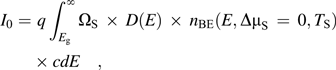 $$I_0 = \,\,q\int_{E_{\rm{g}} }^\infty {\Omega _{\rm{S}} } \, \times \,D(E)\, \times \,n_{{\rm{BE}}} (E,\Delta {\rm{\mu }}_{\rm{S}} \, = \,0,T_{\rm{S}} ) \times cdE\quad,$$
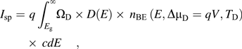 $$ I_{{\rm{sp}}} = \,\,q\int_{E_{\rm{g}} }^\infty \!{\Omega _{\rm{D}} } \times D(E) \times \,n_{{\rm{BE}}} \,(E,\Delta {\rm{\mu }}_{\rm{D}} = qV,T_{\rm{D}} )\, \times \,cdE,$$
 $$P_{{\rm{in}}} =\, \,q\int_{E_{\rm{g}} }^\infty {\Omega _{\rm{S}} } \, \times \,D(E)\, \times \,n_{{\rm{BE}}} \,(E,\Delta {\rm{\mu }}_{\rm{S}} \, = \,0,T_{\rm{S}} )\, \times \,cEdE\quad.$$
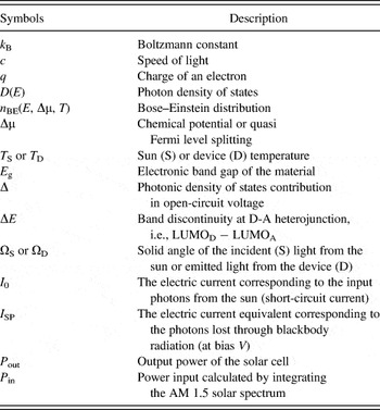
Here, D(E) is the photon density of states, n BE is the Bose–Einstein distribution, ΩS is the solid angle of the incident radiation from the sun, and ΩD is the solid angle of reemission from solar cells.Reference Shockley and Queisser28, Reference Polman and Atwater29 This angle mismatch is fundamental to loss of open-circuit voltage in solar cells,Reference Khan and Alam30 as:
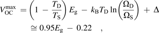 $$V_{{\rm{OC}}}^{\max } \, = \,\left( {1\, - \,{{T_{\rm{D}} } \over {T_{\rm{S}} }}} \right)\,E_{\rm{g}} \, - \,k_{\rm{B}} T_{\rm{D}} \ln \left( {{{\Omega _{\rm{D}} } \over {\Omega _{\rm{S}} }}} \right)\, + \,\Delta \cong 0.95E_{\rm{g}} \, - \,0.22\quad,$$
where the first, second, and third terms are related to Carnot loss, angle entropy loss, and photonic density of state,Reference Hirst and Ekins‐Daukes31 respectively. At room temperature, the right-hand side of Eq. (1e) anticipates the maximum open-circuit voltage within ∼2% of those obtained from the numerical solution of SQ equations. The calculation also shows that FFmax < 0.92 for solar materials with E g ≤ 2 eV.Reference Khan and Alam30 We wish to emphasize that the constraints of, and hold true to all types of solar cell technologyReference Hirst and Ekins‐Daukes31, Reference Green32 and not specific to excitonic PV.Reference Hirst and Ekins‐Daukes31, Reference Green32 Indeed, the angle entropy loss is implicit in all numerical calculationsReference Tress, Petrich, Hummert, Hein, Leo and Riede33 or explicit in analytical formulation.Reference Shockley and Queisser28, Reference Polman and Atwater29 In addition, V OC can be further degraded (i.e., V OC <  $V_{{\rm{OC}}}^{{\rm{max}}} $) through nonradiative recombination and other loss mechanisms.
As already discussed, a BHJ-OPV differs from a classical solar cell because the discontinuity at the heterojunction, i.e., ΔE (≡ LUMOD − LUMOA), is essential for cell operation, and therefore, the classical SQ formula must be adapted accordingly for BHJ-OPV. The photons are still absorbed at ΔE G (≡ LUMOD − LUMOA), but they recombine at primarily at the D/A interface with cross-gap ΔE HL ≡ LUMOA − HOMOD ≡ E G − ΔE, see Fig. 1(c). This reduction in emission band gap increases the dark current and reduces efficiency. In other words, Eq. (1c) should now be rewritten asReference Khan and Alam30:
 $$I_{{\rm{sp}}}^{{\rm{BHJ}}} = \,q\int_{E_{{\rm{HL}}} }^\infty \!{\Omega _{\rm{D}} } \times \,D(E) \times n_{{\rm{BE}}} \,(E,\Delta {\rm{\mu }}_{\rm{D}} = qV,T_{\rm{D}} )\, \times \,cdE\quad.$$
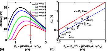
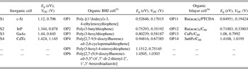
Figure 2(a) shows the OPV-specific “SQ limit” for donor/acceptor OPV obtained by solving Eqs. (1) and (2). The blue solid line in Fig. 2(b) shows the corresponding thermodynamic limit of V OC [Eq. (1e)], with E G replaced by the cross-gap E HL of donor/acceptor organic semiconductors. Remarkably, the measured V OC (filled square symbols) in OPV is close to its thermodynamic limit. The gap between red and the blue lines is attributed to fundamental angle entropy of the system [last term in Eq. (1e)] that cannot be reduced by exciton engineering. In this regard, V OC of OPV, despite its morphological complexity, is no different from those of inorganic semiconductors, such as Si, GaAs, CIGS, etc. [filled circles, Fig. 2(b)].Reference Green32 As mentioned previously, actual V OC is lower than  $V_{{\rm{OC}}}^{\max } $ due to nonradiative recombination losses.
The SQ efficiency limit for an OPV. (a) When the band discontinuity (ΔE) is small, classical SQ analysis suggests that peak efficiency is obtained close to the band gap of ∼1.45 eV. The band discontinuity between the organic semiconductors reduces efficiency (primarily through a loss in V OC) and shifts the peak efficiency curve to higher band gap. For ΔE = 0.5 eV (magenta line), maximum η occurs at ∼1.7 eV. (b) The relationship between V OC and E G or E HL. Here, E HL is the cross-gap of the OPV and E G is the band gap of elemental semiconductor (e.g., Si, GaAs, CIGS). The blue solid line represents the calculated (theoretical) approximation for V OC at different E HL or E G, see Eq. (1e). The symbols are experimental values obtained from literatureReference Rand, Burk and Forrest34, Reference Scharber, Mühlbacher, Koppe, Denk, Waldauf, Heeger and Brabec35 (see Table II).


Measured open-circuit voltage for organic and inorganic solar cell.

The key to improve V OC (as well as the efficiency) of OPV is to increase the cross-gap E HL ≡ E G − ΔE. Note that for a discontinuity of ΔE (≡ LUMOD − LUMOA) ∼0.7 eV, the limiting efficiency at 2 eV (band gap of light-absorbing P3HT layers) is reduced from ∼25% to ∼13.5%, see Fig. 2(a). This result should be viewed as an upper limit because we have assumed that the thermalization loss and the free energy gain from the band discontinuity (ΔE) are sufficient to dissociate excitons into free electron hole pairs.Reference Giebink, Wiederrecht, Wasielewski and Forrest19 We will now discuss the practical aspects of OPV that reduce the efficiency from ∼13.5% to ∼5% (for P3HT/PCBM system) and evaluate the merits of various strategies for efficiency improvement.
III. MORPHOLOGY-AWARE MODELING OF OPV
The operation of BHJ-OPV depends on coupled transport of photons, excitons, electrons, and holes through complex phase-segregated material under variable electric field.Reference Blom, Mihailetchi, Koster and Markov12–Reference Kirchartz, Taretto and Rau15 Two types of modeling approaches have been used to analyze these phenomena: some groups have focused on calculating the output response of a cell by solving the coupled transport problem in a homogenized effective media approximationReference Blom, Mihailetchi, Koster and Markov12, Reference Koster, Smits, Mihailetchi and Blom36, Reference Clarke and Durrant37 or in an idealized geometry,Reference Sylvester-Hvid, Rettrup and Ratner38, Reference Giebink, Wiederrecht, Wasielewski and Forrest39 while others have focused on the mesoscopic physics of various subprocessesReference Zhu and Kahn40 (e.g., exciton dissociation at the D/A interface) that could potentially be the rate limiting process for charge transport. The effective media approach provides important insights about the impact of various physical parameters (e.g., carrier mobility, active layer thickness, polymer band gap, etc.) on the solar cell performance and explains the experimentally measured I-V characteristics. However, this approach fails to explain the dependence of the I-V characteristics on the device morphologies fabricated under different processing conditions (e.g., annealing, mixing, etc.). Similarly, the modeling work that exclusively focuses on the various subprocesses (e.g., exciton dissociation) can explain the role of heterojunction morphology at the local scale but does not explain the overall cell performance as a function of various morphologies and process conditions. Thus, the existing modeling approaches are not quite suitable for modeling the multiscale problem of OPV physics because both the local and the global morphology are essential to the performance of OPV, and many characteristic features of the OPV would be lost if these aspects are ignored. We believe that a third approach, based on a morphology-aware end-to-end device modelingReference Ray, Nair and Alam17, Reference Ray and Alam24–Reference Dongaonkar, Servaites, Ford, Loser, Moore, Gelfand, Mohseni, Hillhouse, Agrawal, Ratner, Marks, Lundstrom and Alam27 of BHJ-OPV, can provide additional insights. We will discuss this approach below.
A. Processing of an OPV: Phase separation and Ostwald ripening
The first step of end-to-end modeling of OPV involves a theoretical description of the morphology that dictates cell performance.Reference Ray, Nair and Alam17, Reference Ray and Alam24 There have been many recent works on the physical characterization of the BHJ morphology by electron tomography,Reference van Bavel, Sourty, de With and Loos41, Reference Andersson, Herland, Masich and Inganäs42 x-ray diffraction,Reference Mayer, Toney, Scully, Rivnay, Brabec, Scharber, Koppe, Heeney, McCulloch and McGehee16 and other advanced scattering techniques.Reference Chen, Xu, He, Wang, Wang, Strzalka, Liu, Wen, Miller, Chen, Hong, Yu and Darling43 It is now believed that the exact nature of the nanomorphology critically depends on the specific D-A material system. For example, McGehee et al.Reference Mayer, Toney, Scully, Rivnay, Brabec, Scharber, Koppe, Heeney, McCulloch and McGehee16 have shown formation of bimolecular crystals of fullerene, intercalated between the side chains of the semiconducting donor polymers. Depending on the spacing between the side chains of the polymer molecules, the system may either intercalate or mix at the molecular scale (e.g., MDMO-PPV, pBTTT, pTT, etc.) or, alternatively, phase separate at large scale (e.g., P3HT, BEH-BMB-PPV). More recently, Darling et al.Reference Chen, Xu, He, Wang, Wang, Strzalka, Liu, Wen, Miller, Chen, Hong, Yu and Darling43 have shown hierarchical nanomorphology in the PTB7: fullerene system, where nanocrystallite aggregates of fullerene and polymer are observed in the polymer-rich and fullerene-rich domains, respectively. Thus, it is clear that there is no universal rule or form for the complex BHJ morphology, and hence, a complete generic modeling framework that provides precise and universal description of this broad class of morphology is nearly impossible.
The common theme in the processing of BHJ morphology is the blending of the donor–acceptor molecules, which either leads to microscale phase separation (or molecular scale mixing, MDMO-PPV, pBTTT) or macroscale phase separation (or large-scale phase separation, e.g., P3HT). The kinetics of both these processes can be described by the Cahn–Hilliard (C-H) approach, which requires conservation of D/A phases and an appropriate free energy function (f) describing the thermodynamics of the D-A blend. The C-H formalism, however, is a mean field theory: it approximates the composition of D/A phases by an average variable ( $\phi $), and spatially resolved information regarding microphase is not available. The time evolution of phase variable (
 $\phi $) is given by the following C-H equationReference de Gennes44–Reference Jones46:
 $${{\partial {\varphi} } \over {\partial t}}\, = \,M_0 \,\left( {\nabla ^2 {{\partial f} \over {\partial {\varphi} }}\, - \,2\kappa \nabla ^4 {\varphi} } \right)\quad,$$
where  ${\varphi}$(x, y, z, t) is the volume fraction of one of the D/A phases, M 0 is the Onsager mobility coefficient dictated by the polymers and the solvent, and κ is the gradient energy coefficient dictated by interfacial energy between two phases. The free energy function (f) of the homogenized mixture depends on entropy, interaction energy (given by the Flory parameter),Reference de Gennes44, Reference Jones46 and the relative sizes of the organic molecules. The detailed description of the free energy and the computational methodology is described in our previous publications.Reference Ray, Nair and Alam17, Reference Ray and Alam26 In this modeling framework,Reference Ray, Nair and Alam17, Reference Ray and Alam26 we neglect the effects of solvent evaporation and the substrate strain, although substantial work is being done in this regard by a number of groups.Reference Wodo and Ganapathysubramanian47, Reference Shang, Kazmer, Wei, Mead and Barry48 The key limitation of this approach is that it cannot give the spatial distribution of the fullerene molecules within the donor-rich or acceptor-rich domains (mean field approximation), i.e., the model cannot describe the formation of hierarchical morphologyReference Chen, Xu, He, Wang, Wang, Strzalka, Liu, Wen, Miller, Chen, Hong, Yu and Darling43 or formation of BHJ structure starting from bilayer structure.Reference Chen, Liu, Wang, Nakahara and Russell49 However, so long the phase volumes are conserved and interconversion is excluded, the general notion of phase separation (or intermixing) should apply to broad range of organic semiconductors used for OPV, as a unifying feature of this problem. Modeling these microscopic effects may require multicomponent generalization of the C-H equation or Cellular automata approach,Reference Peumans, Uchida and Forrest50 generalization of free energies requiring characterization of broader range of parameters, etc. Indeed, developing such generalized formulation should be an important goal of the field.
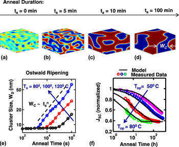
In Fig. 3, we show the simulation results for the morphology evolution during the fabrication process. The initial condition for the simulation is a random mixture with composition fluctuation around the mixing ratio between the two organic components. With anneal duration, as shown in Figs. 3(a)–3(d), the phase segregation of the D-A molecules takes place with the formation of diffused interfaces between the donor-rich (red) and acceptor-rich (blue) domains. Even though the modeling approach is based on several assumptions, the simulated morphology closely resembles the fabricated morphology depicted by tomography and various advanced scattering techniques.Reference van Bavel, Sourty, de With and Loos41–Reference Chen, Xu, He, Wang, Wang, Strzalka, Liu, Wen, Miller, Chen, Hong, Yu and Darling43, Reference Collins, Cochran, Yan, Gann, Hub, Fink, Wang, Schuettfort, McNeill, Chabinyc and Ade51–Reference Hou, Wang, Bergqvist, Andersson, Wang, Müller, Campoy‐Quiles, Andersson, Zhang and Inganäs54
(a–d) Evolution of active layer morphology is plotted with increasing anneal time. We find that the effective width, of the phase-segregated domains scales with anneal time (power-exponent) as shown in (e). The figure also shows that the domain growth is an activated process with strong temperature dependence. Such domain growth is called Oswald ripening and it is a common feature of many polymer/organic blends. (f) The degradation in the short circuit current due to morphology coarsening is plotted. The symbols are experimental data and the solid lines are the model. Details of the model derivation are discussed in Ref. 24.

1. Power law growth of domainsReference Ray and Alam24
The phase-segregated morphology, as shown in Figs. 3(a)–3(d), is a random structure but can be characterized by average domain size, W D, as shown in Fig. 3(d). The average domain size is a statistical quantity, which is numerically computed for a given morphology. In Fig. 3(e), we show the domain size growth with anneal duration. Except for the initial fast transient phase, during which morphology is presumed fractal, the size evolution is determined by the Lifshitz–Slyozov law,Reference Lifshitz and Slyozov23, Reference Jones46 i.e.,  $W_{\rm{D}} \,\tnq#x223C;\,\left[ {M_0 \,f\prime\!\prime\sqrt {\kappa \Delta f} t_{\rm{a}} } \right]^n $, where t a is the anneal time and Δf is the change in free energy. A single parameter (W D) description of the morphology evolution can only be taken as a first-order approximation; phase segregation in real polymer blends is far more complex with crystallization of one phase preceding that of the other,Reference Li, Hu, Fuchs and Chi55 intercalation between the phases,Reference Mayer, Toney, Scully, Rivnay, Brabec, Scharber, Koppe, Heeney, McCulloch and McGehee16 etc. This Lifshitz–Slyozov approximation, however, allows one to calculate the interface area A itf between donor and acceptors. Since the phase volume is conserved, the effective surface area (S) scales as W D(t)A itf(t a) = C or A itf(t a) ∼ (W D)−1 ∼
 $t_{\rm{a}}^{ - n} $. The surface area is the maximum in the well-mixed film, but it reduces as annealing coarsens the film. In our previous work,Reference Ray and Alam24 we have shown that this annealing-dependent coarsening of the morphology can accurately describe the thermal degradation of BHJ-based organic cells, once other mechanisms such as contact degradationReference Schäfer, Petersen, Wagner, Kniprath, Lingenfelser, Zen, Kirchartz, Zimmermann, Würfel, Feng and Mayer56–Reference Krebs59 or interface trap generationReference Bhattacharya, Mayer, Samiee and Dalal60 are minimized. Figure 3(f) shows the close match between the thermal degradation results obtained by measurements (symbols) and predicted by modeling (solid line) based on domain coarsening. Once again, we emphasize that since the approach to morphology evolution described above was primarily developed for polymer–polymer system, it may not accurately or specifically reflect the complex micro- or macrophase segregation of organic polymers. Rather, the results should be viewed as an approximation of the phase segregation process, appropriate for multiscale polymer-to-panel simulation of organic solar cells.
2. Percolation threshold
Mixing ratio between the D-A molecules is an important parameter for the fabrication of high performance organic solar cells.Reference Li, Ray, Alam and Östling22 Experimentally, it has been shown that for a given D-A material pair, there exists an optimum weight ratio for fabricating the most efficient cell.Reference Renz, Keller, Schneider, Shokhovets, Jandt, Gobsch and Hoppe61 The origin of such optimum weight ratio has been recently explained in terms of the degree of intercalation of the fullerene molecules in the side chain of donor polymer.
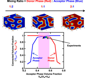
In this work, we show that the optimum weight ratio of organic semiconductors is fundamentally constrained by connectivity of phases to respective contacts, which could in turn be related to percolation theory in 3D random geometry. In Fig. 4, we plot the fractional volume of a given phase (donor: red, acceptor: blue) connected to the appropriate contact, as a function of the volume fraction of the acceptor phase in the mixture. For example, for a donor/acceptor volume mixing ratio of 1:2, the “donor blend phase” (red curve) is fully connected (∼1), but the acceptor phase (blue line) forms islands within the donor phase, and only 60–65% of the acceptor volume is actually connected to the contact. The connectivity maximizes for donor:acceptor ratios of 0.8:1 to 1.25:1 because both volumes are almost 100% connected to the respective contacts. Further increase in donor/acceptor ratio leads to island formation for the donors and rapid loss of connectivity to the contacts.
Optimum mixing ratio (by volume) of donor and acceptor materials. By simulation, we find that 1:1 phase volume ratio ensures that both the donor and acceptor phases form continuous (percolating) pathways for charged carriers between the electrodes. In the figure, V A and V D denote the total volumes of acceptor and donor phases, respectively, and V C,A and V C,Dare the volumes of the acceptor and donor phases connected to both contacts, respectively. The shaded area in the plot shows the desirable volume fraction of the acceptor/donor phases, which ensures almost 100% connectivity for both phases. The experimentally observed optimum mixing ratios (w/w) falls within the shaded window after converting the weight ratios into the phase volume ratios using Eq. (4) for three different donor polymers.

Figure 4 can be interpreted in a two-component percolation framework as follows. It is well known that percolation threshold ( $p_{\rm{c}}^{{\rm{3D}}} $) for an infinite random system is ∼0.3Reference Stauffer and Aharony62; therefore, the donor phase volume ratio must be smaller than 2:1 to form a bicontinuous film without large number of islands. Three additional considerations apply: (i) the real BHJ-OPV cells are neither infinite (thickness ∼100 nm) nor random (phase segregation is correlated); therefore,
 $p_{\rm{c}}^{{\rm{BHJ}}} $ ∼ 0.2 <
 $p_{\rm{c}}^{{\rm{3D}}} $. (ii) On the other hand, conductivity at p c is exponentially suppressed,Reference Stauffer and Aharony62 and quasiohmic transport is restored only at 2 ×
 $p_{\rm{c}}^{{\rm{BHJ}}} $ ∼ 0.4. Finally, (iii) light is primarily absorbed in the donor polymer; therefore, it is desirable to have p D → 0.55 and p A → 0.45. Given these three constraints, it is easy to see why ∼1:1 volume ratio between the donor and acceptor phase gives near optimum performance and moving away from this ratio is so difficult (see Fig. 4).
Finally, one can related the weight ratio to volume ratio using the formula:
 $${{V_{\rm{D}} } \over {V_{\rm{A}} }}\, = \,\left( {{{{\rm{\alpha }}_{{\rm{A}}} - {\rm{\alpha }}_{{\rm{opt}}} } \over {{\rm{\alpha }}_{{\rm{opt}}} - {\rm{\alpha }}_{\rm{D}} }}} \right)\,{{\left( {{1 \over {{\rm{\rho }}_{\rm{D}} }}\, + \,{{{\rm{\alpha }}_{\rm{D}} } \over {{\rm{\rho }}_{\rm{A}} }}} \right)\,} \mathord{\left/ {\vphantom {{\left( {{1 \over {{\rm{\rho }}_{\rm{D}} }}\, + \,{{{\rm{\alpha }}_{\rm{D}} } \over {{\rm{\rho }}_{\rm{A}} }}} \right)\,} {\,\left( {{1 \over {{\rm{\rho }}_{\rm{D}} }}\, + \,{{{\rm{\alpha }}_{\rm{A}} } \over {{\rm{\rho }}_{\rm{A}} }}} \right)}}} \right. \kern-\nulldelimiterspace} {\,\left( {{1 \over {{\rm{\rho }}_{\rm{D}} }}\, + \,{{{\rm{\alpha }}_{\rm{A}} } \over {{\rm{\rho }}_{\rm{A}} }}} \right)}},$$
where ρD and ρA are density of donor and acceptor molecules, αD, αA, and αopt are the weight ratios of fullerene (or PCBM) molecules to donor molecules in donor-rich phase, acceptor-rich phase, and in the active layer, respectively. As shown in Table III (symbols in Fig. 4), despite significant variation in D/A weight ratio, the D/A phase volume ratios are indeed close to those anticipated by the phase connectivity argument.
Relationship between weight ratio (donor molecule:acceptor molecule) and volume ratio (donor phase:acceptor phase). Density of PCBM (ρA) is assumed 1.5 g/cc and the acceptor phase consists of only PCBM.Reference Mayer, Toney, Scully, Rivnay, Brabec, Scharber, Koppe, Heeney, McCulloch and McGehee16

B. The three metrics of practical OPV
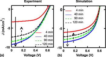
For a given morphology, the output I-V characteristics can be calculated by solving the coupled transport equations for excitons, electrons, and holes. In Fig. 5, we show such I-V characteristics of organic solar cells for different anneal durations. We use drift–diffusion-based transport equations to describe the carrier dynamics in the OPV morphology. It is well known that drift–diffusion does not describe the complex charge transport in soft polymers fullyReference Sylvester-Hvid, Rettrup and Ratner38, Reference Meng, Shang, Li, Li, Zhan, Shuai, Kimber and Walker68, Reference Coffey, Ferguson, Kopidakis and Rumbles69; however, the technique has been widely used as a first-order approximation that captures the essential aspects of the transport problem.Reference Koster, Smits, Mihailetchi and Blom36, Reference Shuttle, Hamilton, O’Regan, Nelson and Durrant70–Reference Buxton and Clarke73 The detailed description of the model equations and the boundary conditions are described in our previous publications.Reference Ray, Nair and Alam17, Reference Ray and Alam26 Here, we report the essence of the morphology-aware transport analysis for BHJ-OPV. Our analysis shows that the empirical features of the key PV matricesReference Renz, Keller, Schneider, Shokhovets, Jandt, Gobsch and Hoppe61, Reference Dutta, Xie, Kumar, Rathi, Ahrenkiel, Galipeau, Qiao and Bommisetty74 (i.e., J SC, V OC, and FF) can be intuitively interpreted in terms of the total interfacial area A itf(t a) between the D-A phases of the BHJ morphology. Similar characterization of the complex morphology with an effective average quantity such as interfacial area or domain width is also reported by various groups.Reference Geens, Martens, Poortmans, Aernouts, Manca, Lutsen, Heremans, Borghs, Mertens and Vanderzande75–Reference Lei, Yao, Kumar, Yang and Ozolins77 The analysis identifies the improvements in materials and device configurations necessary to close the substantial gap between efficiency reported in the literature and the corresponding SQ limit discussed earlier.
Annealing time-dependent I-V characteristics for BHJ cells. (a) Experimentally measuredReference Zeng, Tang and Chen67 I-V and (b) the corresponding simulatedReference Ray, Nair and Alam17 I-V are shown side by side to demonstrate that the simulation captures the trends in the I-V variation.

1. Morphology-dependent short-circuit current
It is easy to calculate the efficiency of the exciton dissociation at the donor/acceptor interface asReference Ray, Nair and Alam17, Reference Ray and Alam24, Reference Ray, Lundstrom and Alam25:
 $$I_{{\rm{ex}}} \,\propto\, G_{{\rm{ex}}} L_{{\rm{ex}}} A_{{\rm{itf}}} \tanh \left( {{{\left\langle {W_{\rm{D}} } \right\rangle } \over {2L_{{\rm{ex}}} }}} \right)\quad,$$
where G ex is the effective exciton generation rate (for details, see Monestier et al.Reference Monestier, Simon, Torchio, Escoubas, Flory, Bailly, de Bettignies, Guillerez and Defranoux78), T D (≡ ηDT film) is the thickness of the donor layer [Fig. 1(a)], with ηD being the donor volume fraction in the active layer of film thickness T film. For sufficiently long anneal time that allows the emergence of abrupt D/A interface, W D ≥ 2L ex and I ex ∼ G exA itf ∼  $t_{\rm{a}}^{ - n} $. In other words, the efficiency of exciton dissociation reduces with anneal time as the morphology coarsens, and many excitons are lost to self-recombination before reaching the interface [as shown in Fig. 4(a)], consistent with the classical view of BHJ operation. Both experimental results and numerical simulations verify this prediction.Reference Ray, Nair and Alam17, Reference Ray and Alam24, Reference Maturovaá, van Bavel, Wienk, Janssen and Kemerink79, Reference Jo, Kim, Na, Yu and Kim80
Equation (4) may suggest that annealing is counterproductive because annealing would coarsen the morphology (i.e., lower A itf), which would lead to lower exciton collection. Morphology coarsening with annealing is not the entire story though; annealing has two other important functions, which improve the device performance. First, one can show via a one-dimensional analysis of the C-H equation that there is a minimum anneal time to sufficiently phase separate the interface boundaries to produce sharp heterobarrier discontinuity.Reference Wodo and Ganapathysubramanian81 The diffused and disordered interface creates interfacial defect states,Reference Bhattacharya, Mayer, Samiee and Dalal60, Reference Street, Schoendorf, Roy and Lee82–Reference Ray and Narasimhan84 which increase the interfacial recombination.Reference Nalwa, Kodali, Ganapathysubramanian and Chaudhary85 Second, although  $J_{{\rm{ex}}} \propto A_{{\rm{itf}}} $, but so is the interface recombination current,Reference Ray, Lundstrom and Alam25 i.e.,
 $J_{{\rm{rec}}} \propto A_{{\rm{itf}}} $ (see Sec. III. B. 2). In other words, while finer morphology improves exciton collection, the proximity of the counterpropagating electron and hole channels enhances recombination at the D/A interface and reduces J SC (= J ex − J rec). The annealing time, therefore, must be optimized to maximize J SC. Experiments show that a properly optimized cell can achieve quantum efficiency approaching 100% at the short-circuit condition.Reference Park, Roy, Beaupre, Cho, Coates, Moon, Moses, Leclerc, Lee and Heeger7
2. Morphology-independent open-circuit voltage
The introduction of BHJ improves  $J_{{\rm{SC}}} ( \propto A_{{\rm{itf}}} )$ dramatically, but remarkably, all empirical evidences suggest that annealing has very little effect on V OC.Reference Ray, Lundstrom and Alam25, Reference Zeng, Tang and Chen67, Reference Ferenczi, Nelson, Belton, Ballantyne, Campoy-Quiles, Braun and Bradley86–Reference Uhrich, Wynands, Olthof, Riede, Leo, Sonntag, Maennig and Pfeiffer88 Again, an appreciation of the unique operation and geometry of the BHJ-OPV resolves the puzzle, as follows.Reference Ray, Lundstrom and Alam25 At the open-circuit condition, the total recombination current (I rec + I dark) cancels the photogeneration current (∼I ex), making the net current zero, see Fig. 6. The recombination current at V OCis given by:
 $$I_{{\rm{rec}}} \, = \,\mathop \int\!\!\!\int \nolimits {\rm{\gamma }}(n_I (z)p_I (z)\, - \,n_{{\rm{int}}}^2 )dS(z)\, \propto\,\, A_{{\rm{itf}}}\quad ,$$
(a) Both the short-circuit current, J SC (right axis), and dark current (or diode reverse saturation current), J 0 (left axis), depend on interfacial area, A itf. Since A BHJ ∼  $t_{\rm{a}}^{ - n} $, both short-circuit current and the dark current reduce with anneal duration. (b) Despite this dramatic change in A BHJ with anneal time, V OCdoes remain insensitive to anneal time. (c) The combination produces an optimized anneal time for maximum efficiency.

where γ is the bimolecular recombination constant, n int is the intrinsic carrier concentration at the D-A interface,  $n(z_I^ + )p(z_I^ - )\, = \,n_{{\rm{int}}}^2 \exp [q(V_{{\rm{OC}}} )/nkT]\, = \,C_2 $, and the integral spans over the entire D/A interface. Since
 $n(z_I^ + )p(z_I^ - )\, = \,C_2 $, independent of the vertical location (z) within the cell, the constant can be taken out of the integral, i.e.,
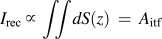 $I_{{\rm{rec}}} \,\propto \,\mathop \int\!\!\!\int\! \nolimits dS(z)\, = \,A_{{\rm{itf}}} $. Since
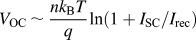 $V_{{\rm{OC}}} \,tnq#x223C;\,{{nk_{\rm{B}} T} \over q}\ln (1 + I_{{\rm{SC}}} /I_{{\rm{rec}}} )$ and both I rec and I SC scale linearly with A itf, V OC does not change significantly with interface area, see Fig. 4(b), and neither annealing nor engineering of the morphology by any other means would affect V OC. The only parameter directly determining the V OC is therefore the cross-gap E HL. This somewhat counterintuitive conclusion is consistent with a broad range of experimental results from the OPV literature.Reference Zeng, Tang and Chen67, Reference Ferenczi, Nelson, Belton, Ballantyne, Campoy-Quiles, Braun and Bradley86–Reference Uhrich, Wynands, Olthof, Riede, Leo, Sonntag, Maennig and Pfeiffer88
3. The μτ product and FF
For a given polymer pair and specific set of electrodes, the cell can be designed so that J SC is close to the theoretical maximum.Reference Park, Roy, Beaupre, Cho, Coates, Moon, Moses, Leclerc, Lee and Heeger7 And, as discussed in Sec. III. B. 2, V OC is dictated by the cross-gap (E HL ≡ E G − ΔE).Reference Ray, Lundstrom and Alam25, Reference Rand, Burk and Forrest34 Therefore, the gap between theoretical SQ efficiency and that of practical BHJ-OPV must be traced to the difference in FF. The “intrinsic FF” reflects the ability of contacts to collect the photogenerated carriers,Reference Tress, Petrich, Hummert, Hein, Leo and Riede33, Reference Andersson, Müller, Badada, Zhang, Würfel and Inganäs89–Reference Bakulin, Rao, Pavelyev, van Loosdrecht, Pshenichnikov, Niedzialek, Cornil, Beljonne and Friend93 especially at low-field, when the cell is forward biased to achieve maximum power output. Although FF can ideally reach 0.9, the experimentally reported FFBHJ values for P3HT:PCBM are in the range of ∼0.5–0.6.Reference Gupta, Mukhopadhyay and Narayan94 The origin of the low FF can be understood as follows.
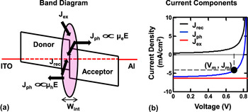
The voltage dependence of the photocurrent, which decides the FF in OPV, is generally explained by the field-dependent charger transfer (CT) exciton dissociation models.Reference Mihailetchi, Koster, Hummelen and Blom95, Reference Limpinsel, Wagenpfahl, Mingebach, Deibel and Dyakonov96 Recently, it has been shown by various groupsReference Tress, Petrich, Hummert, Hein, Leo and Riede33, Reference Andersson, Müller, Badada, Zhang, Würfel and Inganäs89–Reference Bakulin, Rao, Pavelyev, van Loosdrecht, Pshenichnikov, Niedzialek, Cornil, Beljonne and Friend93 that the CT excitons almost invariably lead to free charge carriers, and hence, voltage-dependent photocurrent (and hence the FF) is dictated by the recombination of the free charges at the D-A interfaces. This can be understood more clearly from the band diagram shown in Fig. 7(a), where we show the various current fluxes originating at the D-A interfaces. Here, J ex is the exciton diffusion flux or the rate of charge generation, J ph is the photocurrent or the rate of charge extraction, and J rec is the recombination rate at the interface, such that J ex ≡ J ph(V) + J rec(V). See Fig. 7(a) for the definition of these current components and Fig. 7(b) plots the results from numerical simulation. Since excitons are neutral, exciton flux (J ex) is voltage independent (red line) and it is determined by total absorption and exciton diffusion length. The photocurrent [blue line in Fig. 7(b)] is predominantly the drift currentReference Limpinsel, Wagenpfahl, Mingebach, Deibel and Dyakonov96–Reference Petersen, Kirchartz and Wagner98 dictated by the electric field and the mobility, i.e., J ph = qnIμE = qnIν d. Here, ν d is the drift velocity and nI is the free carrier density at D-A interface. Similarly, the recombination current [black line in Fig. 7(b)] is proportional to the recombination speed at the interface, given by ν rec = W int/τrec. Here, W int is the effective width (∼1 nm) of the interface and τrec is the charge recombination time. For bimolecular recombination mechanism, τrec is inversely proportional to the bimolecular recombination coefficient (γ). Thus, the voltage dependence of the photocurrent can be expressed as  $J_{{\rm{ph}}} (V)\, = \,\left( {{{v_{\rm{d}} } \over {v_{\rm{d}} \, + \,v_{{\rm{rec}}} }}} \right)J_{{\rm{ex}}} \, = \,\left( {{{{\rm{\mu \tau }}E} \over {{\rm{\mu \tau }}E \,+\, W_{{\mathop{\rm int}} } }}} \right)J_{{\rm{ex}}} $. Here, the electric field ≈ (V bi − V)/T film, where V bi is the built-in voltage defined by the work function of the electrodes and V is the operating voltage. At short-circuit condition, V = 0 V, so that E is high and J ph(V = 0) ∼ J ex—the efficiency of carrier collection is high. At maximum power point (V = V m), electric field is suppressed, so that J ph(V) ∼ μτEJ ex/W int, which suggests that even with perfect exciton dissociation at the D/A interface, the poor μτ product (typical of polymers and polymer interfaces) ensures dramatic reduction of the total photocurrent close to maximum power point, leading to empirically observed low FF. The expression for J ph(V) suggests that the FFBHJ can be improved with higher mobility polymersReference Minemawari, Yamada, Matsui, Tsutsumi, Haas, Chiba, Kumai and Hasegawa99, Reference Northrup100 or improved quality of interface that suppresses recombination (higher τrec), strategies that we will discuss below.
Various current fluxes at the heterointerface of OPV. (a) Typical OPV band diagram with the current fluxes indicated by arrows. (b) Components of the J-V characteristics of a BHJ-OPV. The maximum power point in the J-V curve is indicated as dark circle. The maximum power point current and voltage are denoted by J m and V m, respectively. The low FF of the BHJ-OPV (blue line) is attributed to rapid increase in J rec(black line) at the maximum power point of the J-V curve.

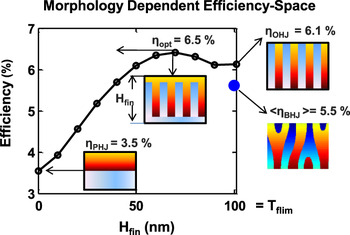
Design space for optimum templated morphology (FIN-OPV), showing optimal morphology (see ηopt). For Hfin = 0, the structure corresponds to Planar Heterojunction (see ηPHJ) cell; and for Hfin = T film, it becomes Ordered Heterojunction (see ηOHJ), as shown. The plot shows the efficiency variation of FIN-OPV as a function of Fin height, while keeping Fin width constant at Wfin = 1.5Lex.

IV. STRATEGIES FOR EFFICIENCY ENHANCEMENT
The organic semiconductors used in OPV literature are often characterized by unique morphology and nature of carrier transport could vary depending on specific technologies. Nevertheless, the generic theory of BHJ-OPV discussed can help us assess the prospects of several strategies of performance improvement suggested by several groupsReference McGehee101–Reference Berson, de Bettignies, Bailly, Guillerez and Jousselme103 in the recent past to improve OPV efficiency, as discussed next.
A. Improved efficiency from morphology engineering
There is a perception that regularized fin-like morphology based on top-down templated heterostructure (Fig. 8)Reference McGehee101, Reference Gorodetsky, Chiu, Schiros, Palma, Cox, Jia, Sattler, Kymissis, Steigerwald and Nuckolls102 or self-assembled kinetically trapped morphologies like double gyroids could fundamentally improve PV efficiency by providing connected conduction channels to the respective contacts for every electron/hole generated by exciton dissociation. Indeed, two-dimensional (2D) cross-sectional images of a random phase-segregated morphology do show a large number of electrically isolated islands that appears to contribute to extinction of exciton, without contributing to J ph.
Like a network in “plumber’s nightmare,” a 2D cut provides an incomplete representation of the 3D system. Elementary results from percolation theory suggest that the notion of random 1:1 structure containing a large number of islands is flawed. Since the percolation threshold of a 3D thin film is expected to be substantially below the bulk value of ∼0.3, a typical ∼1:1 mixture cannot have a significant number of islands.Reference Mayer, Toney, Scully, Rivnay, Brabec, Scharber, Koppe, Heeney, McCulloch and McGehee16 Indeed, it would be difficult to explain ∼100% quantum efficiencyReference Park, Roy, Beaupre, Cho, Coates, Moon, Moses, Leclerc, Lee and Heeger7 in BHJ-OPV, if exciton quenching in isolated islands led to substantial loss in photocurrent. We have recently shown that “random morphology is close to optimum” and morphology engineering does not yield substantial benefits in terms of performance or variability (Fig. 8).Reference Ray and Alam26
The kinetically trapped morphology and/or templated structures, however, may improve long-term thermal stability. A key stability concern for solution-processed BHJ-OPV fabricated at low temperature is its propensity for phase segregation even at operating conditions.Reference Ray and Alam24 If optimized for peak efficiency before installation, a dramatic degradation in efficiency is expected (and has been experimentally observed) during operation. In this regard, the top-down template structure may improve thermal stability of the film and increase the lifetime of the solar cells.
B. Approaches for improved mobility or suppressed recombination
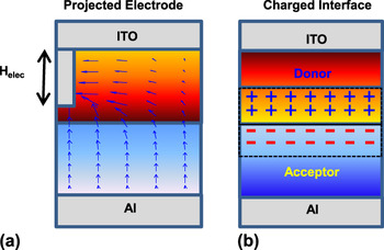
Numerical simulations show that improving mobility increases FF substantially.Reference Ray and Alam26 A wide variety of ideas have been offered but none without important drawbacks. For example, improving crystallinity improves mobility of a polymer,Reference Minemawari, Yamada, Matsui, Tsutsumi, Haas, Chiba, Kumai and Hasegawa99 but the film may no longer be processable in solution. Percolation doping by carbon nanotubesReference Berson, de Bettignies, Bailly, Guillerez and Jousselme103 or nanostructured electrodesReference Nam104–Reference Bhattacharya, Chakravarty, Pattnaik, Dennis Slafer, Biswas and Dalal107 are expected to reduce the path lengths of charge collection and improve FF [Fig. 9(a)]; however, the initial results are inconclusive. In fact, theoretical calculations show that if these electrodes breach the junction, J rec may be substantially enhanced, and the efficiency gain is completely lost. Finally, there have been several recent efforts to reduce recombination at the interface.Reference Tada, Geng, Wei, Hashimoto and Tajima108–Reference Yuan, Reece, Sharma, Poddar, Ducharme, Gruverman, Yang and Huang110 This technique appears promising, but adaptability to BHJ-OPV remains an open question. As an alternative to mobility enhancement, one can also try to suppress interfacial recombination by introducing a thin charged layer [Fig. 9(b)] at the D-A interface, so that the free carriers are pushed away from the interface and the recombination is suppressed. Initial theoretical calculation suggests that this approach may increase the FF dramatically to ∼80%.Reference Ray and Alam111 While similar concepts have been demonstrated for planar heterojunction cells,Reference Tada, Geng, Wei, Hashimoto and Tajima108 its feasibility for BHJ-OPV is yet to be demonstrated.
New device concepts for the improvement of the FF in OPV. (a) Inserted electrode for better charge collection. (b) Implanted fixed charge layers at the interface to reduce interfacial charge recombination.

C. Low band gap and low cross-gap materials
The HOMO–LUMO gap of a typical polymer in use today ranges between 1.7 and 1.9 eV, and many researchers feel that lowering the band gap to 1.2–1.5 eV may improve J SC and efficiency. In a recent article, NelsonReference Nelson5 summarizes various techniques to develop low band gap polymers such as planarization of the polymer backbone, addition of heteroatoms, alternating electron-rich units with electron-poor units in a push–pull configuration, etc. Figure 2, however, shows that for typical band discontinuity of ΔE (≡ LUMOD − LUMOA) ∼ 0.5 eV, the change in bulk band gap E G (≡ LUMOD − HOMOD) does not improve efficiency significantly. Instead, it is more important to reduce the band discontinuity between the HOMO level of the donor polymer and LUMO level of the acceptor polymer, i.e., increase the cross-gap between the polymer pairs. Efforts to lower band discontinuity by either increasing the LUMO level of PCBM by adding various side chains or decreasing HOMO level of P3HT by replacing C with Si have already been demonstrated. Finally, an approach based on including low band gap dye at the D/A interface seems promising,Reference Honda, Ohkita, Benten and Ito112 but the efficiency gain by this approach needs to be quantified.
The efficiency enhancement strategies, as reviewed in this section, focus on improving the intrinsic material or device properties and hence must be implemented at cell level. To translate these improvements into higher panel efficiencies, we must also identify and minimize the parasitic losses responsible for reducing the panel efficiency. In Sec. V, we outline a combined device–circuit approach for capturing theses aspects and discuss the insights it offers.
V. ORIGIN OF POOR PANEL EFFICIENCY IN OPV
A common challenge for all PV technologies is the loss of efficiency when cells are connected in series to create the solar panel. This gap between cell and panel efficiency is universal for all technologies, including OPV, where panel aperture area efficiencies are as low as 2–3%.Reference Jin, Tao, Velusamy, Aljada, Zhang, Hambsch, Burn and Meredith113–Reference Krebs, Gevorgyan, Gholamkhass, Holdcroft, Schlenker, Thompson, Thompson, Olson, Ginley, Shaheen, Alshareef, Murphy, Youngblood, Heston, Reynolds, Jia, Laird, Tuladhar, Dane, Atienzar, Nelson, Kroon, Wienk, Janssen, Tvingstedt, Zhang, Andersson, Inganäs, Lira-Cantu, de Bettignies, Guillerez, Aernouts, Cheyns, Lutsen, Zimmermann, Würfel, Niggemann, Schleiermacher, Liska, Grätzel, Lianos, Katz, Lohwasser and Jannon115 There are many factors responsible for this loss in efficiency at the panel level, arising from challenges in large area deposition of thin absorber and contact layers, while using low temperature high throughput processes. The two major loss mechanisms responsible for this gap between cell and panel are resistive losses in the transparent conducting oxide (TCO) layer and losses due to parasitic local shunt currents, distributed across the cell surface. These loss mechanisms are common to all solar cell technologiesReference Dongaonkar, Servaites, Ford, Loser, Moore, Gelfand, Mohseni, Hillhouse, Agrawal, Ratner, Marks, Lundstrom and Alam27, Reference Dongaonkar, Karthik, Mahapatra and Alam116–Reference Wolden, Kurtin, Baxter, Repins, Shaheen, Torvik, Rockett, Fthenakis and Aydil118 and, as we show in this section, account for a large percentage of panel efficiency loss. To analyze the panel efficiency, we use an equivalent circuit approach, which allows us to represent small individual cells using equivalent circuits, and connect them in series and parallel to form a panel.Reference Dongaonkar, Servaites, Ford, Loser, Moore, Gelfand, Mohseni, Hillhouse, Agrawal, Ratner, Marks, Lundstrom and Alam27, Reference Dongaonkar, Karthik, Mahapatra and Alam116–Reference Wolden, Kurtin, Baxter, Repins, Shaheen, Torvik, Rockett, Fthenakis and Aydil118
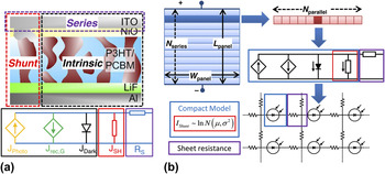
The intrinsic I-V characteristics obtained from the modeling approach discussed in the preceding sections can be used for analyzing small laboratory-scale cells (see Fig. 5). To simulate panel characteristics, however, we need to use an equivalent circuit framework, as shown in Fig. 10(a). This can incorporate the intrinsic physics of generation and recombination inside the cell, as well as the physics and statistics of parasitic shunts, and contact sheet resistance, as shown in Fig. 10(a). In thin film solar cells, the shunt current shows a power law voltage dependence, which can be understood as a localized space-charge-limited shunt path, in parallel to diode current.Reference Dongaonkar, Servaites, Ford, Loser, Moore, Gelfand, Mohseni, Hillhouse, Agrawal, Ratner, Marks, Lundstrom and Alam27 These shunt defects are distributed spatially randomly on the cell surface, with their magnitudes showing a lognormal distribution.Reference Dongaonkar, Karthik, Mahapatra and Alam116
(a) Schematic of an organic BHJ solar cell, showing the intrinsic region, parasitic shunt, and contact series resistance regions. These components are captured in the compact model shown at the bottom, with the various generation and recombination fluxes, as well as the parasitic components. (b) (clockwise from top) Schematic representation of the SPICE simulation approach for a typical thin film PV panel with N series cells in series, subdivided into N parallel subcells, each of which is represented by the equivalent circuit in part (a). This circuit incorporates the relevant physics as well as the statistical distribution of shunt current magnitude (red box). Finally, we obtain the 2D network of equivalent circuit for simulating panel performance.

To quantify the impact of these parasitic effects at panel level, we create an equivalent circuit of the panel, by using the cell equivalent circuit shown in Fig. 10(a). As shown in Fig. 10(b), for a typical thin film PV panel with N series cells in series, we divide individual cells into 1 × 1 cm subcells, which are connected in series and parallel using the TCO sheet resistance to form a panel equivalent circuit.Reference Dongaonkar and Alam117 Each subcell is represented by an equivalent circuit with different shunt current values, obtained from the measured lognormal distribution of shunt current values [Fig. 10(b)]. This approach enables us to carry out and end-to-end (i.e., process–device–panel) simulation, by including the effect of parasitic loss mechanisms.
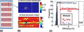
Figure 11(a) shows the schematic of a typical OPV panel, with geometrical dimensions obtained from data sheets of Konarka® Technologies (Lowell, MA). We use the circuit approach discussed above and assign varying shunt current values to each subcell, as shown in Fig. 11(bi). We assume that all other properties of the subcells are identical, except for the variation in parasitic shunt current. The subcell efficiency without any shunt losses is assumed to be 5%, a typical value for a high quality P3HT:PCBM cell. We can now simulate the whole panel circuit using SPICE and explore the effect of shunt variability on module performance. The impact of such randomly distributed shunts can be understood from Fig. 11(bii), which shows the power output of individual subcells when the panel is operating at its maximum power point. Note that the highly shunted subcell (highlighted) actually consumes the power produced in the neighboring regions and has a disproportionately large impact on panel efficiency. This illustrates the importance of these correlated effects when cells are connected to form modules. The module efficiency is not a simple average of various cell efficiencies but is determined by these effects related to interconnection and biasing.
(a) Schematic of an OPV solar panel from Konarka® Technologies showing rows of thin wide solar cells connected in series, with current direction as shown. (b) Simulation of series connected cells showing lognormally distributed shunt current values (for 10 cells). (i) The defective cell with high shunt current (circled) and direction of current flow are marked. (ii) Power output of individual subcells showing that the shunted cells affecting neighboring regions in parallel (c) Monte Carlo simulations of panel efficiency, comparing champion cell efficiency (black line), with the distribution of panel efficiencies (histogram), clearly separating the resistive losses (red line) from shunt variability losses (magenta).

To get a more quantitative assessment of these losses, we also perform Monte Carlo simulations of panel efficiency in presence of random shunt defects and calculate the panel efficiency distribution for a given shunt distribution, as shown in Fig. 11(c). Note that for best subcell efficiency of 5%,Reference Li, Shrotriya, Huang, Yao, Moriarty, Emery and Yang10, Reference Ma, Yang, Gong, Lee and Heeger11, Reference Kim, Liu, Namboothiry and Carroll119 the panel efficiency reduces to 2.7–3% for typical module dimensions.Reference Jin, Tao, Velusamy, Aljada, Zhang, Hambsch, Burn and Meredith113–Reference Krebs, Gevorgyan, Gholamkhass, Holdcroft, Schlenker, Thompson, Thompson, Olson, Ginley, Shaheen, Alshareef, Murphy, Youngblood, Heston, Reynolds, Jia, Laird, Tuladhar, Dane, Atienzar, Nelson, Kroon, Wienk, Janssen, Tvingstedt, Zhang, Andersson, Inganäs, Lira-Cantu, de Bettignies, Guillerez, Aernouts, Cheyns, Lutsen, Zimmermann, Würfel, Niggemann, Schleiermacher, Liska, Grätzel, Lianos, Katz, Lohwasser and Jannon115 The simulation also servers to highlight the respective contribution to panel efficiency loss from contact sheet resistance (about 1.6% absolute) and the shunt current variability (about 0.5% absolute). This gap between cell and module efficiency in OPV is fairly consistent with other PV technologies.Reference Wolden, Kurtin, Baxter, Repins, Shaheen, Torvik, Rockett, Fthenakis and Aydil118
In this analysis, we have analyzed the losses due to shunt variability, due to its universal nature and availability of robust statistical data.Reference Dongaonkar, Servaites, Ford, Loser, Moore, Gelfand, Mohseni, Hillhouse, Agrawal, Ratner, Marks, Lundstrom and Alam27, Reference Dongaonkar, Karthik, Mahapatra and Alam116, Reference Dongaonkar and Alam117 The SPICE framework used, however, is very general and can be easily adapted to analyze other sources of variability and panel level losses. This analysis highlights the “practical” efficiency limit of the OPV panels because of the inevitable shunt and series resistance losses. And, in addition to the various strategies for efficiency improvement at the cell level, mitigation of these losses will require an enhanced emphasis on improvement in TCO properties and improved process control in manufacturing.
VI. PROGNOSIS AND CONCLUSION
The analysis in this paper leads to a number of surprising conclusions regarding the efficiency of BHJ-OPV from cell to panel level.
(i) A simple derivation of the thermodynamic limit of efficiency for BHJ-OPV shows that while the band gap discontinuity (ΔE) between donor/acceptor material is essential for exciton dissociation, it is also responsible for loss of intrinsic efficiency below the classical SQ limit, ηSQ(E G) >
 ${\rm{\eta }}_{{\rm{SQ}}}^{{\rm{BHJ}}} $ (E G, ΔE).
(ii) The
${\rm{\eta }}_{{\rm{SQ}}}^{{\rm{BHJ}}} $ (E G, ΔE) limit is yet to be achieved in practice. A combination of process modeling and a coupled solution of exciton, electron, and hole transport traces this difference in efficiency to low FF arising from poor mobility of polymers and high recombination at the D/A interface; otherwise, J SC is already close to maximum limit and V OC cannot be changed with morphology engineering.(iii) Various approaches to improve mobility (e.g., crystalline, projected electrode, doping by nanowires or nanotubes) are being explored and could improve performance—however, each approach also has important drawbacks whose implication should be understood in a comprehensive framework.
(iv) Our use of 3D percolation theory suggests that (a) random morphology is close to optimum, i.e., the performance of OPV cannot increase significantly with regularizing the structure and that (b) the volume ratio cannot significantly deviate from 1:1 mixture.
(v) We find that efficiency improvement requires that we simultaneously reduce E G and band discontinuity ΔE. Unless ΔE is reduced significantly, exclusive focus on band gap reduction may not improve efficiency significantly.
(vi) Finally, we used combined device–circuit simulations to study the practical constraints in translating OPV cell efficiency to panel efficiency. The analysis points to the dominant role of contact sheet resistance and random shunt defects in reducing the panel level performance.


Despite the constraints of morphology and transport discussed in this article, the low cost of solution-processed polymers and the impressive increase in efficiency over the last decade suggests bright prospects of OPV in applications like building-integrated PV where its low-cost unique form factor, reduced weight, semitransparency, “aesthetics appeal” may not be matched by more traditional PV technologies.
Supplementary Material
Supplementary materials can be viewed in this issue of the Journal of Materials Research by visiting http://journals.cambridge.org/jmr.
ACKNOWLEDGMENTS
The work was supported by the Center for Re-Defining Photovoltaic Efficiency through Molecule Scale Control, an Energy Frontier Research Center funded by the U.S. Department of Energy, Office of Science, and Office of Basic Energy Sciences under Award No. DE-SC0001085.