



Introduction
Geologic studies concerning ice-sheet extent and directions of ice movement constitute an important branch of Quaternary research (e.g., Stokes et al., Reference Stokes, Tarasov, Blomdin, Cronin, Fisher, Gyllencreutz and Hättestrand2015). They allow us to understand the mechanism of advance and retreat of ice sheets during individual glaciations. The digital elevation model (DEM) has become a particularly useful tool for this type of research (Clark, Reference Clark1997; Jorgensen and Piotrowski, Reference Jorgensen and Piotrowski2003; Raunholm et al., Reference Raunholm, Sejrup and Larsen2003; Ewertowski and Rzeszewski, Reference Ewertowski and Rzeszewski2006; King et al., Reference King, Pritchard and Smith2016; Rychel and Morawski, Reference Rychel and Morawski2017; Teodorski, Reference Teodorski2023). However, there are cases (e.g., connected with postglacial processes like erosion) in which the glacial relief is not well developed enough to make conclusions about the directions of the ice-sheet movement. A second useful method for determining the local direction of ice-sheet movement is the analysis of pebble fabric in tills. The use of this method, however, has a major limitation, because it depends on the number of till exposures available. The textural features of the tills, indicated by the arrangement of the pebbles, are also present in the microscale. An effective tool for measuring the average orientation of fine grains is the anisotropy of magnetic susceptibility (AMS) method, which has been used to determine not only the directions of movement, but also the mechanism of ice-sheet movement, and to reconstruct processes of subglacial till formation. This method of studying tills has been refined across more than six decades of use (e.g., Fuller, Reference Fuller1962; Stupavsky and Gravenor, Reference Stupavsky and Gravenor1975; Stewart et al., Reference Stewart, Bryant and Sweat1988; Hooyer et al., Reference Hooyer, Iverson, Lagroix and Thomason2008; Thomason and Iverson, Reference Thomason and Iverson2009; Gentoso et al., Reference Gentoso, Evenson, Kodama, Iverson, Alley, Berti and Kozlowski2012; Fleming et al., Reference Fleming, Stevenson and Petronis2013; Tylmann et al., Reference Tylmann, Wysota and Piotrowski2013; Ankerstjerne et al., Reference Ankerstjerne, Iverson and Lagroix2015; Król and Wachecka-Kotkowska, Reference Król and Wachecka-Kotkowska2015; Hopkins et al. Reference Hopkins, Kleman, Evenson and Kodama2016; McCracken et al., Reference McCracken, Iverson, Benediktsson, Schomacker, Zoet, Johnson, Hooyer and Ingólfsson2016; Narloch et al., Reference Narloch, Werner and Tylmann2021; Teodorski et al., Reference Teodorski, Dzierżek and Ziółkowski2021).
The aim of this research was to reconstruct the directions of ice advance and pattern of its retreat during the Saalian (Marine Isotope Stage [MIS] 6) and Upper Stadial of the Weichselian (MIS 2) glaciation in the study area in north-central Poland. The AMS method was used for the study, supported by the DEM analysis. An original method of collecting AMS till samples from the areas of glacial plateaus was used. This quick method of sampling, combined with the further development of the AMS measurement technique, makes it possible to determine the directions of ice-sheet movement in any area with near-surface layers of glacial tills and where there are no exposures of these tills. The results of the research provided new information on the glacial history of this part of Poland, in particular on the extent, direction of movement, advance, and retreat of ice sheets during the Saalian and Weichselian glaciations.
Geomorphological and geological settings
The research area is located in north-central Poland. Its eastern part belongs to the Płońsk Plateau (Fig. 1B), which is part of the North Mazovian Lowland (Solon et al., Reference Solon, Borzyszkowski, Bidłasik, Richling, Badora, Balon and Brzezińska-Wójcik2018). Elevation ranges here from 114 m above sea level (asl) in the northern part, adjacent to the Raciąż Plain, to 164 m asl in the central part, and it drops again toward the south to 84 m asl. Most of the study area is a glacial plateau. Small areas are occupied by fluvioglacial deposits, mainly in the western (south of Sierpc), central (east of Staroźreby), and southern (northwest of Wyszogród) parts of the area. Several sequences of terminal moraines have also been identified in this region.
(A) Location of the study area (green rectangle) against the extent of the ice sheet during the Saalian (S) and Weichselian (W) glaciations and their directions of ice-sheet movement (after Marks et al., Reference Marks, Dzierżek, Janiszewski, Kaczorowski, Lindner, Majecka, Makos, Szymanek, Tołoczko-Pasek and Woronko2016, Reference Marks, Karabanov, Nitychoruk, Bahdasarau, Krzywicki, Majecka and Pochocka-Szwarc2018, Reference Marks, Bitinas, Błaszkiewicz, Börner, Guobyte, Rinterknecht, Tylmann, Palacios, Hughes, García-Ruiz and Andrés2022); (B) geomorphological map of the study area. LGM, the maximum extent of the Weichselian glaciation ice sheet (according to Dzierżek, Reference Dzierżek2009; Marks et al., Reference Marks, Bitinas, Błaszkiewicz, Börner, Guobyte, Rinterknecht, Tylmann, Palacios, Hughes, García-Ruiz and Andrés2022); K.-D. sph., Kujawy–Dobrzyń subphase (after Niewiarowski et al., Reference Niewiarowski, Olszewski and Wysota1995).

The western part of the study area belongs to the Dobrzyń Lakeland (Fig. 1B), which is part of the Chełmno-Dobrzyń Lakeland (Solon et al., Reference Solon, Borzyszkowski, Bidłasik, Richling, Badora, Balon and Brzezińska-Wójcik2018). Elevation in this region ranges from 57 to 146 m asl. It is also a glacial plateau, except for small fragments of land in the western and southern parts that are occupied by fluvioglacial deposits. The characteristic elements of the glacial relief of the Dobrzyń Lakeland are numerous arcs of terminal moraines that have been described by many other researchers (e.g., Nechay, Reference Nechay1927; Lamparski, Reference Lamparski and Kostrzewski1991; Dzierżek, Reference Dzierżek2009; Teodorski, Reference Teodorski2023). They mark the location of the paleo–ice sheet front during the last deglaciation. Another characteristic element of the glacial relief is a conspicuous network of glacial meltwater channels.
Both areas of glacial plateau are separated from each other by the Urszulewo Plain, also belonging to the Chełmno-Dobrzyń Lakeland (Solon et al., Reference Solon, Borzyszkowski, Bidłasik, Richling, Badora, Balon and Brzezińska-Wójcik2018; Fig. 1B). Its flat surface slopes from north to south, from 135 to 81 m asl. It is an outwash plain built of fluvioglacial deposits.
The area of the Płońsk Plateau was last covered by an ice sheet during the Warta stadial of the Saalian glaciation (MIS 6) (Marks et al., Reference Marks, Dzierżek, Janiszewski, Kaczorowski, Lindner, Majecka, Makos, Szymanek, Tołoczko-Pasek and Woronko2016; Fig. 1A). Several sequences of terminal moraines occur here, reflecting successive stages of ice-sheet recession. Moraine hills are known from the area north of Wyszogród, near Staroźreby or Raciąż (Baraniecka, Reference Baraniecka1996; Kacprzak and Lisicki, Reference Kacprzak and Lisicki2005; Kucharska and Wasiluk, Reference Kucharska and Wasiluk2005; Frankiewicz, Reference Frankiewicz2009; Różański and Włodek, Reference Różański and Włodek2009; Fig. 1B). In the west, they occur between the villages of Kurowo, Mochcino, and Bielsk (Lamparski, Reference Lamparski1978; Dzierżek, Reference Dzierżek2009).
The western part of the study area (Dobrzyń Lakeland and Urszulewo Plain) was last covered by the Płock Lobe of the Weichselian ice sheet (Rühle, Reference Rühle1957; Skompski, Reference Skompski1969; Marks, Reference Marks1988, Reference Marks2022; Mojski, Reference Mojski2005; Dzierżek, Reference Dzierżek2009; Roman, Reference Roman2010; Marks et al., Reference Marks, Dzierżek, Janiszewski, Kaczorowski, Lindner, Majecka, Makos, Szymanek, Tołoczko-Pasek and Woronko2016; Fig. 1A). The last glacial maximum (LGM) in this part of Poland falls in the Poznań phase, dated to 20–19 ka (Marks et al., Reference Marks, Dzierżek, Janiszewski, Kaczorowski, Lindner, Majecka, Makos, Szymanek, Tołoczko-Pasek and Woronko2016, Reference Marks, Bitinas, Błaszkiewicz, Börner, Guobyte, Rinterknecht, Tylmann, Palacios, Hughes, García-Ruiz and Andrés2022). On the other hand, the latest 10Be exposure dating shows that the local LGM in western and central Poland is ca. 25–21 ka, and ice-sheet retreat from the extent of Poznań phase began at 17.3 ± 0.5 ka (Tylmann et al., Reference Tylmann, Rinterknecht, Woźniak, Bourlès, Schimmelpfennig and Guillou2019). The Poznań phase is correlated with the Frankfurt phase in Germany and the Grūda phase in Lithuania (Marks, Reference Marks2012). The extent of the ice sheet during the local LGM is not definitive at this time, due to the few hills of terminal moraines that could confirm its extent. According to Kotarbiński (Reference Kotarbiński1998), in the area of Sierpc and to the north of it (outside the study area), there are single moraine hills that were deposited during the Weichselian glaciation. Dzierżek (Reference Dzierżek2009) indicates the existence of terminal moraines from the local LGM period on the Mochcino-Kurowo line (Fig. 1B), which was also pointed out by Lamparski (Reference Lamparski1978). Roman (Reference Roman2019) reconstructs the extent of the last ice sheet based on moraines in Mikołajewo (east of Płock) and moraine hills northwest of Mochcino, as well as the distribution of outwash plains. She also indicates the presence of overridden moraines in the hinterland of the local LGM ice limit, which were originally formed before the maximum extent of the ice sheet during the Weichselian glaciation. Różański and Włodek (Reference Różański and Włodek2009) also draw attention to the existence of moraines in Mikołajewo. In the Urszulewo Plain, due to meltwater erosion and accumulation of fluvioglacial sediments, it is difficult to trace the successive recessional limits of the ice sheet. Roman (Reference Roman2019) recognized the presence of overridden moraines from the pre-maximum period in the area to the northwest of Płock. Numerous sequences of terminal moraines in the Dobrzyń Lakeland reflect the extent of individual glacial lobes that formed during successive phases of the last deglaciation (Lamparski, Reference Lamparski and Kostrzewski1991, Reference Lamparski and Dzierżek2001; Dzierżek, Reference Dzierżek2009; Teodorski, Reference Teodorski2023). Moraines in the northern part of the region indicate the extent of the transgressive–regressive Kujawy–Dobrzyń subphase (Fig. 1B), which has been dated at 17.7 ka BP (Kozarski, Reference Kozarski1995; Wysota et al., Reference Wysota, Lankauf, Szmańda, Chruścińska, Oczkowski and Przegiętka2002).
The tills forming the surface parts of the study area were examined. The Płońsk Plateau is built of sediments belonging to the Saalian glaciation. The thickness of these sediments exceeds 100–110 m in the central part of the plateau (Kacprzak and Lisicki, Reference Kacprzak and Lisicki2011; Różański and Włodek, Reference Różański and Włodek2012). These are mainly glacial tills, ice-dammed sediments, and fluvioglacial sands and gravels (e.g., layers 3–14 of profile I–J in Fig. 2). Glacial tills belonging to the Warta Stadial of the Saalian glaciation are exposed on the terrain surface (MIS 6; Baraniecka, Reference Baraniecka1996; Frankiewicz, Reference Frankiewicz2009; Kacprzak and Lisicki, Reference Kacprzak and Lisicki2011; Różański and Włodek, Reference Różański and Włodek2012; layer 7 of profile I–J, as well as layer 12 of other profiles). They usually reach a thickness of several meters, up to a maximum of 30–40 m in the central part of the plateau.
Representative geologic cross sections in the study area (based on Lamparski, Reference Lamparski1980, Reference Lamparski1985; Dzierżek, Reference Dzierżek2006; Różański and Włodek, Reference Różański and Włodek2012; Frankiewicz, Reference Frankiewicz2013). Locations of the cross sections on the Fig. 4. Elsterian Glaciation (MIS 12): 1-glacial tills; Holsteinian Interglacial (MIS 11): 2-fluvial sands with gravels, sands, silts and clays; Saalian Glaciation, Main Stadia! (MIS 6): 3-fluvioglacial sands, 4-glacial tills; Saalian Glaciation, Warta Stadia! (MIS 6): 5-fluvioglacial sands and gravels, 6-ice-dammed silts and clays, 7-glacial tills, 8-ice-dammed sands and silts, 9-fluvioglacial sands and gravels, 10-silts, sands and clays of kames, 11-fluvioglacial sands and gravels, 12-glacial tills, 13-ice-dammed sands and silts, 14-fluvioglacial sands with gravels; Eemian Interglacial (MIS 5e): 15-limnic silts, gyttjas and peats, 16-fluvial sands and gravels, 17-fluvial sands and silts; Weichselian Glaciation, Middle Stadia! (MIS 4): 18-glacial tills, 19-ice-dammed clays; Weichselian Glaciation, Upper Stadia! (MIS 2): 20-fluvioglacial sands, 21-ice-dammed silts and sands; 22-glacial tills, 23-fluvioglacial sands, 24-limnic and fluvial silts, sandy clays and sands; 25-glacial tills; 26-sands and gravels of moraine hills; 27-fluvioglacial sands and gravels; 28-sands and silts of kames and kame terraces; 29-tills, gravels and silts of glacial curvilineations; 30-flow tills; 31-fluvioglacial sands; 32-limnic sands; 33-fluvial sands, gravels and silts; Weichselian Glaciation/Holocene (MIS 2/MIS 1): 34-limnic and fluvial sands and silts; Holocene MIS 1 : 35-fluvial sands; 36-muds; 37-peats.
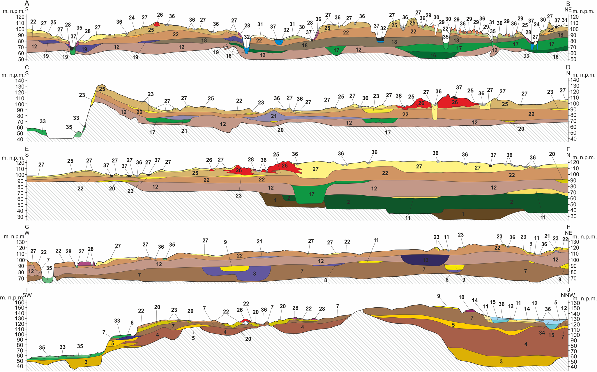
The Dobrzyń Lakeland and Urszulewo Plain areas are built of sediments accumulated during the Weichselian glaciation. In the Lakeland area, these deposits reach from several meters (in the northern and western parts; Lamparski, Reference Lamparski1985; Dzierżek, Reference Dzierżek2006) to more than 70 m, north of Mochowo (Dzierżek and Szymanek, Reference Dzierżek and Szymanek2009) and mainly consist of glacial tills, ice-dammed sediments, and fluvioglacial sands and gravels. On the profiles in Figure 2, the sediments belonging to the Weichselian glaciation are represented by layers 18–33. Glacial tills deposited during the Upper Stadial of the Weichselian glaciation are exposed on the surface of the glacial plateau (MIS 2; Lamparski, Reference Lamparski1978, Reference Lamparski1980, Reference Lamparski1985; Dzierżek, Reference Dzierżek2006; Różański and Włodek, Reference Różański and Włodek2012). The thickness of these tills generally reaches 15 m.
Methods
Analysis of the DEM
The DEM used for the study was generated on the point cloud basis with a horizontal resolution of 1 m, obtained on the basis of light detection and ranging (LIDAR) scanning of the terrain surface. Elevation data come from the resources of the Head Office of Geodesy and Cartography in Warsaw. QGIS 3 was used to generate the model. To determine the origin of the glacial forms, individual sheets of the Detailed Geological Map of Poland at the scale of 1:50,000 were analyzed (Mojski, Reference Mojski1958; Skompski and Słowański, Reference Skompski and Słowański1962; Skompski, Reference Skompski1968; Łyczewska, Reference Łyczewska1973; Lamparski, Reference Lamparski1978, Reference Lamparski1980, Reference Lamparski1985; Baraniecka, Reference Baraniecka1996; Kotarbiński, Reference Kotarbiński1998; Kacprzak and Lisicki, Reference Kacprzak and Lisicki2005; Kucharska and Wasiluk, Reference Kucharska and Wasiluk2005; Dzierżek, Reference Dzierżek2006; Wysota, Reference Wysota2006; Dzierżek and Szymanek, Reference Dzierżek and Szymanek2009; Frankiewicz, Reference Frankiewicz2009; Różański and Włodek, Reference Różański and Włodek2009; Wysota and Sokołowski, Reference Wysota and Sokołowski2009). The analysis of the DEM was carried out for the purpose of determining the orientations of glacial landforms in the study area.
Grain-size analysis
Wet-sieving tests (Mycielska-Dowgiałło and Rutkowski, Reference Mycielska-Dowgiałło and Rutkowski1995) were carried out on 33 samples of glacial tills at 1.5–2.0 m depths. A sample weighing 200 g, taken from drilling samples, was sieved under running water on a set of 11 sieves with the following diameters: 10, 4, 2, 1, 0.8, 0.355, 0.2, 0.125, 0.1, and 0.063 mm.
Petrographic analysis of the gravel fraction (5–10 mm)
Thirty-three samples of glacial till at 1.5–2.0 m depths and weighing 2 kg, taken from drilling samples, were used for the study, from which a gravel fraction with a diameter of 5–10 mm was separated. From each sample, at least 100 grains were analyzed (according to the procedure of Lisicki [Reference Lisicki2003]), which were classified as Scandinavian rocks (crystalline rocks and northern quartz, limestones, dolomites, sandstones and quartzites, and northern shales) or local rocks (limestones and marls, sandstones, mudstones, and claystones, as well as other local rocks like flints and lydites). Due to the vast predominance of crystalline rocks and/or northern limestones and small percentage changes in other types of rocks, only two main types of rocks are described in the results.
Collection of AMS samples
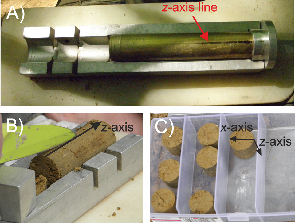
AMS samples were taken from near-surface layers of glacial tills forming areas of postglacial plateau. The sampling procedure was as follows: (1) drilling a maximum depth of 2 m using a handheld Eijkelkamp probe (two to three drilling holes per site), (2) AMS sampling using a 15-cm-long and 2.54-cm-diameter brass sampler (Fig. 3A) from a depth of 1.5–2.0 m, driven vertically into the bottom of the hole. This sampling depth was adopted due to the possible disturbance of sediments in the upper layers as a result of frost processes or biogenic or human activity. Unfortunately, the handheld Eijkelkamp probe does not allow tracing any undisturbed sedimentary structures of tills located above 2 m depth. The z-axis line and the direction of the north were marked on the brass sampler. Before the probe was removed from the hole, the azimuth and the angle of inclination of the probe axis were measured. Then, the till cores were pushed out from the sampler. The obtained till cores were cut to the standard size for AMS cylindrical specimens (2 cm long and 2.54 cm wide; Fig. 3B and C). They were oriented relative to a 3D coordinate system with z- and x-axes marked on their surfaces. On average, two to five AMS samples were obtained from one core, and four cores in two to three drilling holes were obtained from each site. In this particular site, each hole is about 1–2 m away from the next one. The total number of samples collected was 458 pieces.
Examples of anisotropy of magnetic susceptibility (AMS) sample collection: (A) brass sampler with z-axis line and north direction (black line); (B) till core with z-axis line on the top; (C) individual AMS samples with z- and x-axes line.
Anisotropy of magnetic susceptibility (AMS)
The AMS of the samples was measured using the MFK1-FA Kappabridge (Agico) with a 3D rotator and Safyr 7 software. Magnetic susceptibility measurements were carried out in a field with an intensity of 200 A/m and a frequency of 976 kHz. AMS measurements were carried out at the European Center for Geological Education in Chęciny (Poland).
To visualize the data, stereographic projections to the lower hemisphere in the geographic coordinate system generated with Anisoft 5 were used. The projections show the orientation of the principal axes of magnetic susceptibility—maximum (k max), intermediate (k int), and minimum (k min). The mean orientations of the individual susceptibility axes with their confidence ellipsoids were calculated on the basis of Jelínek (Reference Jelínek1978). To describe the susceptibility and its anisotropy for individual samples, the following parameters were calculated: mean magnetic susceptibility [K m = (k max + k int + k min)/3]; magnetic lineation [L = k max/k int]; magnetic foliation [F = k int/k min]; corrected degree of anisotropy [Pj = (k max/k min)a], where a = √(1 + T 2/3); and the shape parameter [T = (2η 2 − η 1 − η 3)/(η 1 − η 3)], where η 1 = ln k max, η 2 = ln k int, η 3 = ln k min (Hrouda, Reference Hrouda1982). Before the AMS projection was interpreted, the available results were filtered. The values K m and Pj were selected for filtration. The filtration was based on the median and 25% and 75% quartiles. Samples above the level described by the formula Q3 + 1.5 × IQR, where Q3 is the 75% quartile, and IQR is the interquartile range between the 25% and 75% quartiles, were removed due to anomalously high values of the parameters (Hodge and Austin, Reference Hodge and Austin2004; Stachowska et al., Reference Stachowska, Łoziński, Śmigielski, Wysocka, Jankowski and Ziółkowski2020; Teodorski et al., Reference Teodorski, Dzierżek and Ziółkowski2021). The IQR outliers method is not dependent on abnormally high boundary values, unlike the standard deviation method. This method depends only on the 25th and 75th percentiles, which means that it measures the spread of the middle 50% of the results of a given set. According to this author, this method allows for better filtration of abnormally high AMS parameter values. A sample with such high AMS parameter values can significantly affect the magnetic fabric of a given site. Extremely high parameter values may be associated, for example, with the occurrence of rock fragments with high AMS anisotropy. As a result of filtration, 68 samples were removed, which is about 15% of all measured samples. The obtained AMS results were subjected to statistical analysis that consisted of determining the degree of spatial orientation of the maximum and minimum magnetic susceptibility axes. For each set of orientations of the susceptibility axes, the eigenvector v 1 was determined (Woodcock, Reference Woodcock1977), which estimates the mean direction of the axes and the eigenvalue of this vector, λ 1. To determine the grouping of the axes around the mean vector, the normalized eigenvalues S 1 were calculated based on the formula S 1 = λ 1/N, where S 1 < 1 (Woodcock, Reference Woodcock1977). In the present paper, it was assumed that certain statistically mean directions of the susceptibility axis are obtained when S 1 ≥ 0.6. When S 1 is below 0.6, the axes are poorly oriented. However, if the determined direction is confirmed by the orientation of glacial landforms, it is used in the interpretation with caution. In addition, the value of the S 1 eigenvalue for the orientation of the maximum susceptibility axis may indicate the magnitude of the action of shear forces during the deposition of glacial tills (Hooyer et al., Reference Hooyer, Iverson, Lagroix and Thomason2008).
Rock magnetism analysis
The selected AMS samples were used for all rock magnetism analyses. For the initial determination of the type of magnetic minerals, S-ratio measurements were carried out. In the first step, a magnetic field of 1 T (IRM1T), was applied along the z-axis, followed by an inverse field of 100 mT (IRM−100mT). The S-ratio was calculated according to the formula S = −(IRM−100mT/IRM1T) (Stober and Thomson, Reference Stober and Thompson1979; Grabowski et al., Reference Grabowski, Bakhmutov, Kdýr, Krobicki, Pruner, Rehákowá, Schnabl, Stoykova and Wierzbowski2019). Thirty-three samples were used for the measurements, one from each location. Measurements of the stepwise acquisition of isothermal remanent magnetization (IRM) were carried out on six samples with different S-ratio values and from different locations. The magnetic field was applied to the samples along the z-axis in 22 steps of magnetization up to a maximum field value of 3 T. Both analyses allow for determining the relationship of low-coercivity minerals (e.g., magnetite) to high-coercivity minerals (e.g., hematite, goethite) (e.g., Opdyke and Channell, Reference Opdyke and Channell1996).
The Lowrie test (Lowrie, Reference Lowrie1990) was carried out on 10 samples from different locations and with different S-ratio values. Magnetic fields of 1.4 T, 0.4 T, and 0.1 T along the z-, y-, and x-axes were applied to the samples. The samples were then thermally demagnetized in 13 steps, up to 700°C. This test allows for the identification of magnetic minerals on the basis of their Curie temperatures, with the division into minerals with different coercivity.
Anisotropy of anhysteretic remanent magnetization (AARM) was carried out on 25 samples from three locations differing in the T parameter value. The ARM was applied in 12 specific directions. In the analysis, an alternating field in the range of 0−100 mT and a steady field of 100 μT were used. After each cycle of ARM measurements, the samples were demagnetized. An analysis was conducted to determine the types of minerals responsible for AMS (Jackson, Reference Jackson1991).
The magnetic remanent was applied with the LDA5/PAM1 (Agico) pulse magnetizer/demagnetizer for ARM and the MMPM 10 pulse magnetizer (Magnetic Measurements) for IRM. Magnetic remanent was measured using a JR-6A (Agico) spinner magnetometer with Rema 6 software. Measurements of rock magnetism were carried out at the European Center for Geological Education in Chęciny (Poland).
Results
Location and orientation of moraine sequences
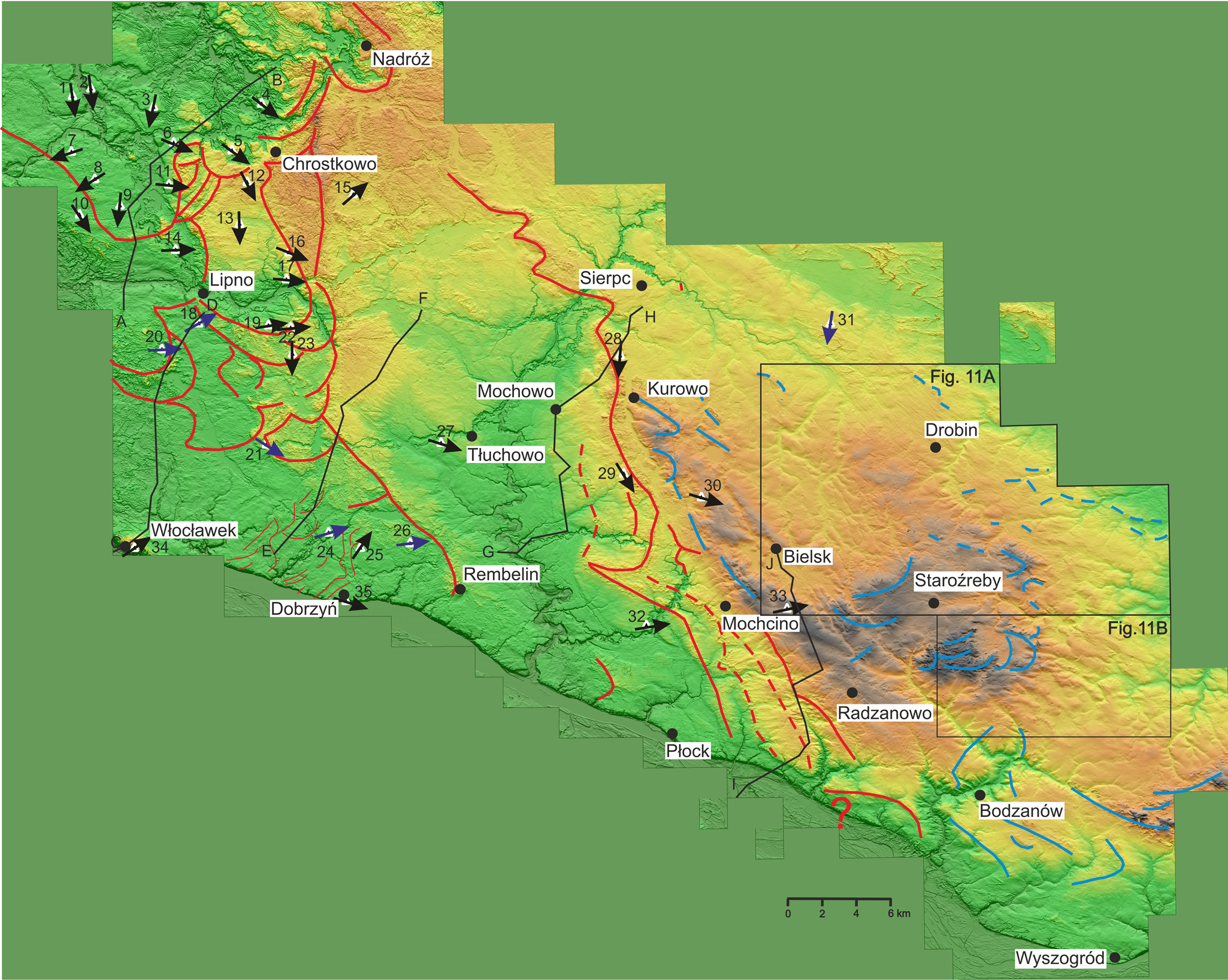
Several sequences of terminal moraines have been marked out in the area of the Płońsk Plateau. In the SE part of the research area, to the northeast of Wyszogród, there are clearly visible, generally latitudinally oriented moraine hills up to 30 m high (Fig. 4). These moraines are probably extended by the remains of moraine hills near Bodzanów. Another series of terminal moraine hills, although poorly visible on the DEM, is located in the NE part of the study area, southeast of Drobin. It is generally oriented latitudinally, and the maximum height of the hills is 8 m. It shows the extent of the ice-sheet front in the younger recessive episode of the Saalian glaciation. Moraines in the central part of the Płońsk Plateau, near Staroźreby, are characterized by an orientation similar to NE-SW. The highest moraine hills reach 28 m in height. Then, farther west, between Mochcino and Kurowo, there are more moraines belonging to the Saalian glaciation. They are oriented along the NNW-SEE line and reach a height of up to 14 m.
Location of the anisotropy of magnetic susceptibility (AMS) sites (triangles) along with the interpreted direction of ice-sheet movement (arrows: black are S 1 ≥ 0.6, well oriented axes; blue are S 1 < 0.6, weakly oriented axes) against the background of the digital elevation model (DEM) and the location of sequences of terminal moraine forms (continuous lines, sequences of terminal moraines; dashed lines, sequences of overridden moraines; blue lines, sequences of moraines from the Saalian glaciation; red lines, sequences of moraines from the Weichselian glaciation); see Table 1 for names and numbers of sites.
Anisotropy of magnetic susceptibility (AMS) measurement results.a

a Abbreviations/parameters: na, number of all samples taken; nf, number of samples after filtration; Km, mean magnetic susceptibility; L, magnetic lineation; F, magnetic foliation; Pj, corrected degree of anisotropy; T, shape parameter; mean orientation of principal susceptibility axes: D, declination; I, inclination; k max, maximum susceptibility axis; k int, intermediate susceptibility axis, k min, minimum susceptibility axis; S 1, normalized eigenvalue for the susceptibility axis; IDSM, interpreted azimuth of the direction of ice-sheet movement; (SI), magnetic susceptibility unit; (-), unitless.
b Sites where the S 1 eigenvalue for the k max and k min axes are below 0.6 (weakly oriented axes) have been marked in red.
In the western part of the Płońsk Plateau, several moraine sequences have been preserved, the formation of which can be associated with the local LGM either directly before or after this period (Fig. 4). Between Mochcino, Radzanowo, and Płock, four sequences of forms have been preserved, reflecting the extent and shape of the front of the ice sheet. The first one is located west of Radzanowo, but it is not clearly visible in the terrain. This series includes moraines identified by Różański and Włodek (Reference Różański and Włodek2009) southwest of Radzanowo. The extension of these forms may be fragmentary remains of moraines preserved to the northwest of Mochcino, measuring up to 11 m high. The next two sequences of forms located south and west of Mochcino (Fig. 4, dashed line) have a different character. In addition to the NW-SE lines of forms visible in the DEM and up to 10 m high, they are also characterized by the occurrence of a series of elongated hillocks perpendicular to the main lines of forms. The elongated perpendicular hills reach a height of up to 6 m. Similar sequences of forms, although much more badly preserved, have been identified south of Mochowo. The last and longest series of moraine hills is the most legible in the relief. It begins its course near the Vistula valley, east of Płock. It continues toward the NNW, between Mochowo and Kurowo. Then, at the height of Sierpc, it changes its course to NW-SE. In the southern part, it is less well preserved, reaching up to 11 m in height. On the DEM, it is clearly visible in the northern part, and the hills reach a height of up to 18 m. At some point, this sequence disappears under the fluvioglacial formations accumulated in the later phase of the ice-sheet extent. On the Urszulewo Plain, between Rembelin and Płock, only fragmentary forms have survived, which may be the remains of moraines.
Numerous arcs of terminal moraines have been preserved in the Dobrzyń Lakeland, described in detail in Teodorski (Reference Teodorski2023). Generally, in the southern part of the lakeland, the most visible and longest moraine sequence begins in Rembelin and continues to the northwest (Fig. 4). Moraines in this sequence reach up to 15 m in height. North of Dobrzyń, a number of minor end moraines have been interpreted. Moraine hills are most common in the central part of the lakeland. Moraine arcs are characterized by orientation: W-E and WSW-ENE in the southeast, from NE-SW to N-S in the east, and also close to N-S in the west. The moraines in the eastern part of the area are best visible on the model, and they reach a height of up to 17 m. In the northern part of the lakeland, there is a clear sequence of terminal moraines representing the ice limit of three glacial lobes from the Kujawy–Dobrzyń subphase. The lines of these forms are generally oriented on the WSW-ENE line and reach up to 28 m in height.
Grain-size characteristics and petrography of the gravel fraction of glacial tills
The analyzed tills from the sites covered by this research do not show large differences in terms of granulometry. The content of the gravel fraction ranges from 0.29% (Kamień Kotowy, site 27) to 3.63% (Ignackowo, site 20). The content of the sand fraction ranges from 39.53% (Kikoł, site 11) to 57.83% (Sumin, site 9). The exception is the site in Wawrzonkowo (site 8), where the content of this fraction is 15.01%. The total content of the silt and clay fraction ranges from 41.51% to 60.08%, again except at the site in Wawrzonkowo (site 8), where it is 84.67%. In the gravel fraction with a diameter of 5–10 mm, crystalline rocks constitute 33–34% in the southern part of the Dobrzyń Lakeland, 36–44% in the eastern sites in the study area, 48–66% in the northern part of the Dobrzyń Lakeland, and 34–81% in the central part of the Dobrzyń Lakeland. Northern limestones and other carbonate rocks are essentially absent in the northern and central parts of the Dobrzyń Lakeland (except for the sites in Makowiska, site 10; Chlebowo, site 13; and Ignackowo, site 20). In the remaining sites, in most cases, the northern limestone content ranges from 33% to 47%.
AMS
The magnetic susceptibility of tills in the studied sites ranges from 0.97 × 10⁻⁴ to 2.73 × 10⁻⁴ SI (Table 1). The highest K m was recorded in the northern part of the Dobrzyń Lakeland (2.14 × 10⁻⁴ SI), while the lowest K m was recorded in the Płońsk Plateau, last covered by the ice sheet during the Saalian glaciation (1.4 × 10⁻⁴ SI). In the studied sites, L rarely exceeds 1% and is in the range of 1,000–1,015. The average L values slightly differ in the northern part of the Dobrzyń Lakeland (1.008) and in the Płońsk Plateau (Saalian tills; 1.007). F prevails over L and has a decisive influence on the Pj. The F values for individual stations range from 1,000 to 1,030. The highest average F values were recorded in the southern part of the Dobrzyń Lakeland (1.014) and in the area between the Lakeland and the local LGM extent (1.013). The Pj ranges from 1.003 to 1.038 and reaches the highest values in the regions characterized by the highest F values, assuming the maximum average values of 1.020 (southern part of the Dobrzyń Lakeland). The T parameter has a wide range of values from −0.821 to 0.957. In the northern part of the Dobrzyń Lakeland and in the area covered by an ice sheet during the Saalian glaciation, L prevails (T < 0.0); in the remaining part of the research area, F prevails. The values of S 1 for the mean axis vector k max range from 0.442 to 0.733. S 1 reaches the highest average values in the northern part of the Dobrzyń Lakeland (0.610), and the lowest values in the southern part of the Dobrzyń Lakeland (0.556). The value of S 1 for the k min axis ranges from 0.450 to 0.885.
On the basis of the obtained magnetic fabrics, the directions of the ice-sheet movement were determined (Figs. 4 and 5). When lineation is predominant (T < 0), the direction of ice-sheet movement is determined parallel to the orientation of the k max axis. When foliation prevails in the studied location (T > 0), k max axes are dispersed along a (shear) plane, and AMS fabric has a “girdled” pattern. In this situation, the direction of shear (direction of ice-sheet movement) is parallel to the dip direction of the girdle (or imbrication of k 3 axes) similar to the pebble fabric (Benn, Reference Benn1994; Hooyer et al., Reference Hooyer, Iverson, Lagroix and Thomason2008; Ives and Iverson, Reference Ives and Iverson2019). The girdled pattern of the fabric is characteristic for low shear strain. On the other hand, the AMS fabric is strongly clustered at moderate shear strain (Hooyer et al., Reference Hooyer, Iverson, Lagroix and Thomason2008). In the second case, two subgroups can be distinguished. In the first subgroup of foliated magnetic fabrics, the orientation of k max and k min lies in the direction of ice-sheet movement. The second subgroup concerns fabrics in which the k int and k min axes lie in the direction of ice-sheet movement.
Anisotropy of magnetic susceptibility (AMS) projections in geographic coordinates for individual sites (squares, axis of maximum magnetic susceptibility; triangles, axis of intermediate magnetic susceptibility; circles, axis of minimum magnetic susceptibility) together with the interpreted direction of ice-sheet movement (arrows); red arrows indicate cases where S 1 for the maximum and minimum axes is below 0.6 (weakly oriented axes); see Table 1 for names and numbers of sites.
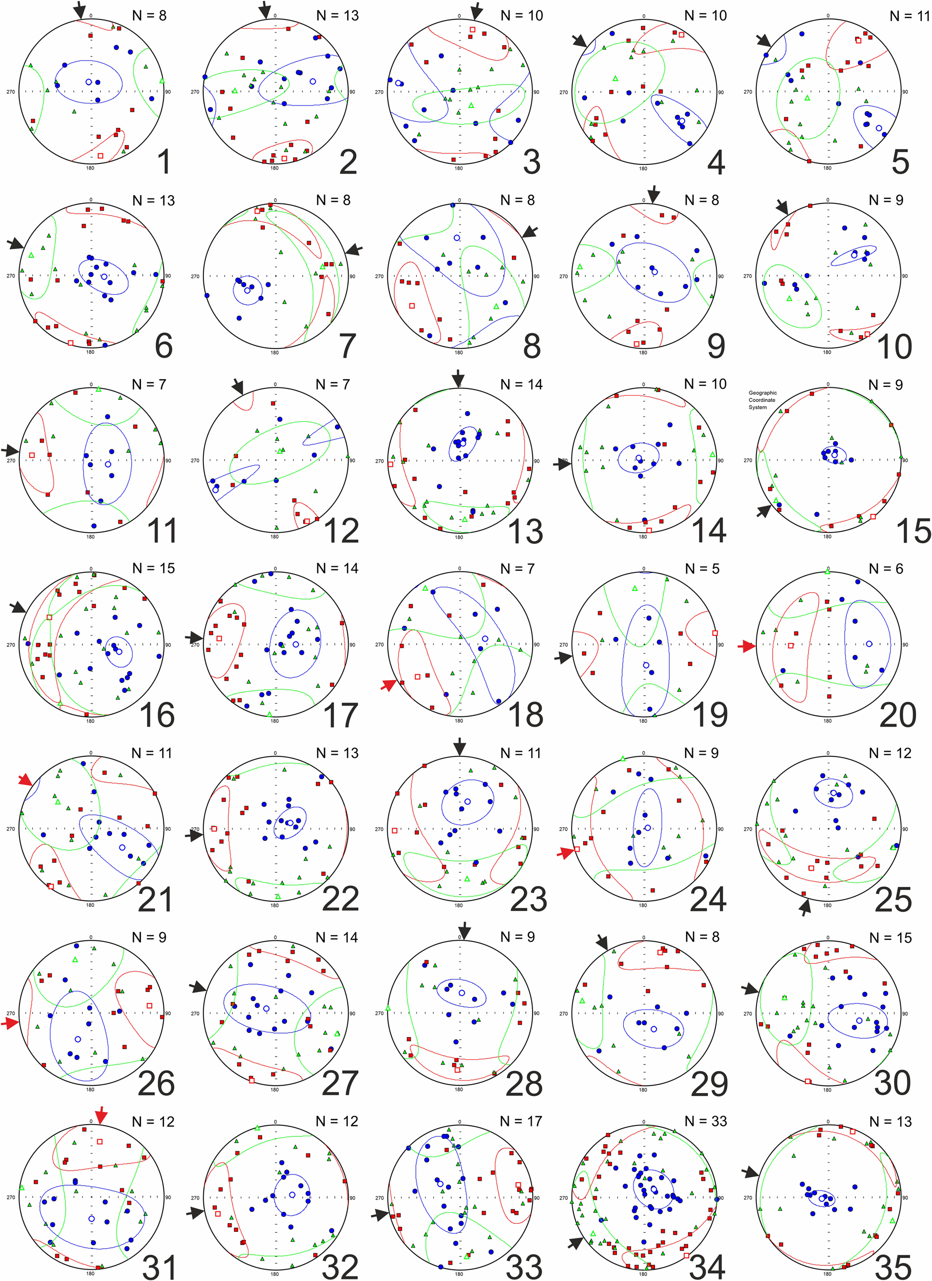
The orientations of the mean vector of individual magnetic susceptibility axes are presented in Table 1. In the northern part of the Dobrzyń Lakeland, the ice-sheet movement directions range from ENE-WSW in the western part (Steklin, site 7; Wawrzonkowo, site 8) through N-S in the northern part (Mazowsze, site 1; Kijaszkowo, site 2; Klonowo, site 3) to NW-SE in the eastern part (Nowa Wieś, site 4; Wildno, site 5) (Figs. 4 and 5). In the central part of the lakeland, it generally changes from the NNW-SEE in the north (Makowiska, site 10; Janowo, site 12) to more W-E farther in the south (Złotopole, site 14; Karnkowo, site 17; Głodowo, site 19; Ignackowo, site 20; Bałdowo, site 23). In the southern part of the Dobrzyń Lakeland, three mean directions of ice-sheet movement were recorded: WNW-ESE (Nowa Wieś, site 21; Dobrzyń, site 35), WSW-ENE (Wierznica, site 24; Michałkowo, site 26), and SW-NE (Mokowo, site 25; Włocławek, site 34). In the Urszulewo Plain and the area of the Płońsk Plateau occupied by the Weichselian glaciation ice sheet, the directions of ice-sheet movement obtained range from NNW-SSE (Rempin, site 29) to SW-NE (Łąkie, site 15). Some order can be observed in the part of the Płońsk Plateau occupied by the Saalian glaciation ice sheet. In the northern part, the direction of movement of the ice sheet is similar to the N-S line (Nowe Piastowo, site 28; Zawidz Kościelny, site 31) and then changes to WNW-ESE or WE (Rychacice, site 30; Kuchary-Jeżewo, site 33).
Rock magnetism
The S-ratio assumes similar values in all sites, from −0.18 to 0.42 (Table 1). In most of the sites, this ratio is slightly positive, which indicates a slight predominance of low-coercivity minerals in the tested samples. The IRM saturation curves take a relatively similar shape (Fig. 6). From the curves, it can be seen that 29–68% of low-coercivity minerals (magnetization in the 0–100 mT field range), 21–36% of medium-coercivity minerals (100–400 mT), and 11–39% of high-coercivity minerals (>400 mT) are responsible for the magnetization of the samples. In many cases, samples do not reach full saturation in a field of 3 T.
Isothermal remanent magnetization (IRM) saturation curves. M/Mmax, ratio of magnetization to maximum magnetization; H, value of the applied magnetic field; see Table 1 for names and numbers of sites.

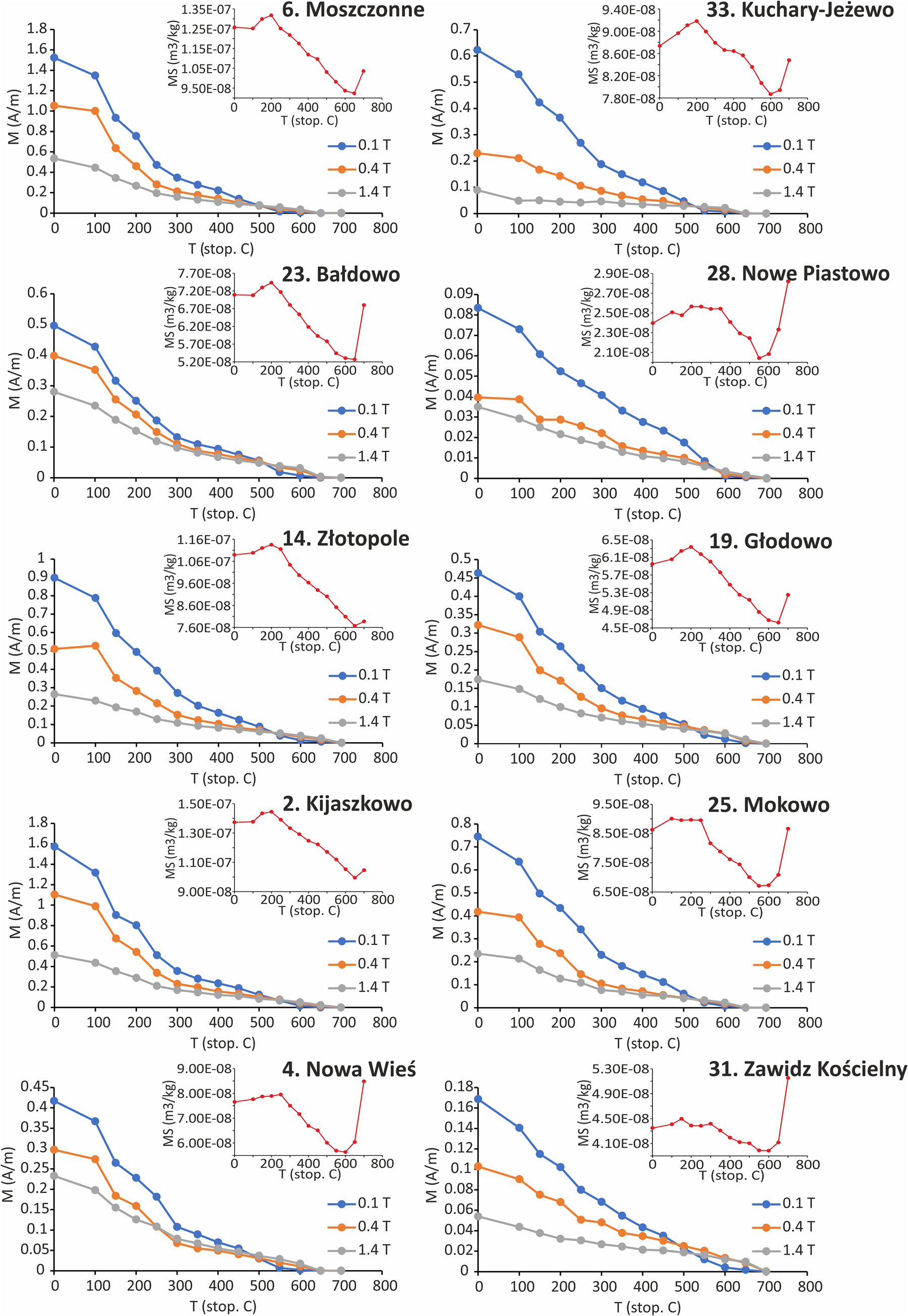
In the Lowrie test, the highest magnetization values can be observed on the x-axis (low-coercivity minerals), although the percentage value of this component is variable (Fig. 7). The samples are completely demagnetized at a temperature of 600–700°C. In many samples (e.g., Nowa Wieś, site 4; Moszczonne, site 6; Bałdowo, site 23), a significant decrease in the magnetic remanent on the x-axis and y-axis is noticeable in the temperature range of 100–300°C. The magnetic susceptibility curve shows an increase in value up to a temperature of 200°C, and then a decrease in its value. A relatively uniform decrease in magnetization to the temperature of 550°C is recorded in the samples from the Nowe Piastowo (site 28), Kuchary-Jeżewo (site 33), and Zawidz Kościelny (site 31).
Lowrie test results (blue line, magnetization on the x-axis; orange line, magnetization on the y-axis; gray line, magnetization on the z-axis) along with the change in magnetic susceptibility during individual heating steps of the samples (red line); see Table 1 for names and numbers of sites.
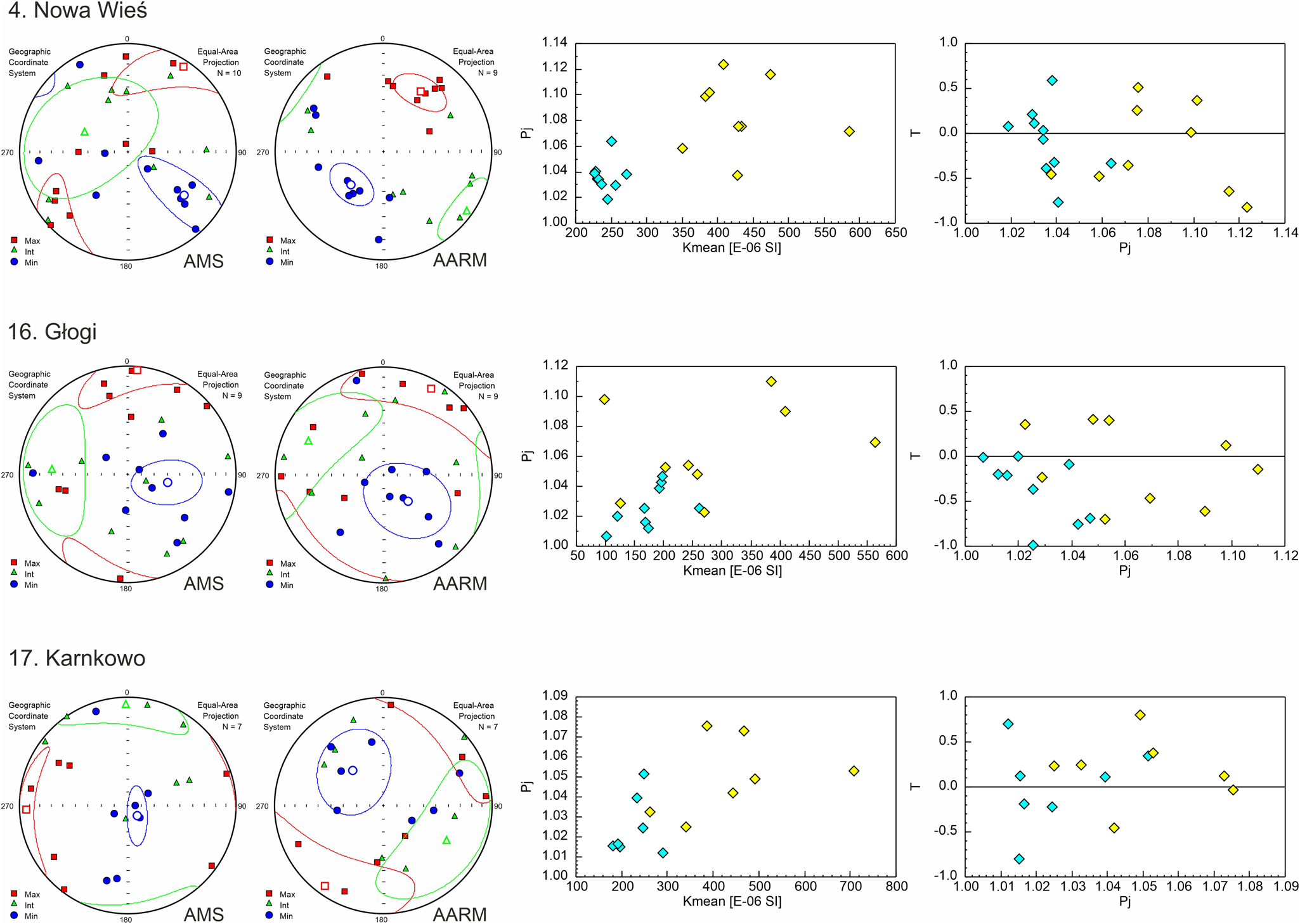
The results of the AARM tests are shown in Figure 8. In the first case (Nowa Wieś, site 4), after using ARM, the AARM axes are more clearly grouped than the AMS axes. The k max azimuth is generally similar, being 33° for AMS and 32° for AARM. Nevertheless, the inclination of the ellipsoid is different in the two cases. In the case of the AMS, the ellipsoid is inclined toward the NW (k int = 293/54), while the AARM ellipsoid is inclined toward the NE (k max = 32/35). In the second case (Głogi, site 16), after using ARM, the AARM axes are less clearly grouped than the AMS axes. In general, the inclination of the AARM axes (k max = 29/10, k int = 294/25, k min = 138/63) relates by direction and inclination to the orientation of the AMS axis (k max = 5/4, k int = 273/31, k min = 102/59). In the third case (Karnkowo, site 17), again after using ARM, the AARM axes are less clearly grouped than the AMS axes. They are also characterized by a different orientation to the AMS and a differently inclined ellipsoid (k max = 216/9, k int = 120/34, k min = 319/55 for AARM; k max = 268/7, k int = 359/8, k min = 138/79 for AMS). In all three cases, the samples after the use of ARM are characterized by higher values of magnetic susceptibility and a much larger spread on the K mversus Pj diagram. In Nowa Wieś (site 4) the parameter T has lower values in AARM (T = −0.192) than in AMS (0.045); in other cases, it has higher values (0.229 and 0.089 for Głogi, site 16, and 0.372 and 0.144 for Karnkowo, site 17, respectively).
Anisotropy of magnetic susceptibility (AMS) and anhysteretic remanent magnetization (AARM) projections for selected sites (squares, axis of maximum magnetic susceptibility; triangles, axis of intermediate magnetic susceptibility; circles, axis of minimum magnetic susceptibility) with K m vs. Pj and Pj vs. T graphs (blue points, AMS data; yellow points, AARM data); see Table 1 for names and numbers of sites.
Discussion
Magnetization carriers
Measurements of the IRM show predominantly low-coercivity minerals and some addition of high-coercivity minerals in the tested till samples (Fig. 6, Table 1).
Based on the Lowrie test (Fig. 7), it was found that magnetite and hematite are present in all tested samples. Hematite is also responsible for the fact that samples do not reach full IRM saturation even at a field of 3 T (Fig. 6). Several minerals may be responsible for the significant decrease in magnetization in the x and y curves seen in many samples. The first explanation for this relationship may be related to the presence of iron sulfides in the tested samples. However, the examined tills showing such a relationship (belonging to the Weichselian glaciation) are characterized by a red-brown color, which indicates the oxidation of iron minerals. The second responsible mineral may be titanomagnetite, which is popular in crystalline rocks included in the studied tills. A third mineral may be maghemite, which Hopkins et al. (Reference Hopkins, Kleman, Evenson and Kodama2016) suggested may account for the marked decrease in magnetization at 200–300°C. Maghemite has been identified in sediments formed in cold environments (Kodama, Reference Kodama1982), including glacial tills (Gentoso et al., Reference Gentoso, Evenson, Kodama, Iverson, Alley, Berti and Kozlowski2012). A clear decrease in magnetization on the x-axis and y-axis at 100–300°C recorded in the samples of tills of the Weichselian glaciation is practically absent in the samples of glacial tills of the Saalian glaciation (Nowe Piastowo, site 28; Zawidz Kościelny, site 31; Kuchary-Jeżewo, site 33). This proves that only magnetite and hematite occur in the tills of the older glaciation.
Comparison of AMS and AARM studies (Fig. 8) indicates that, at least in some sites, AMS is not caused by ferromagnetic minerals but by paramagnetic minerals (Jackson, Reference Jackson1991), most likely lamellar, such as minerals from the mica group or clay minerals. The low magnetic susceptibility of the tested till samples (<5 × 10⁻⁴ SI) may also indicate that magnetic susceptibility may be mainly controlled by paramagnetic minerals (Hrouda, Reference Hrouda, Gubbins and Herrero-Bervera2007). The anisotropy of clay minerals comes from their crystallographic structure. Despite this, it has been proven that magnetic lineations are common in clayey rocks. When cracking along the basic plane, these minerals are arranged parallel to the directions of, for example, stretching (Parés and van der Plujim, Reference Parés and van der Pluijm2002; Cifelli et al. Reference Cifelli, Mattei, Chadima, Hirt and Hansen2005, Reference Cifelli, Mattei, Chadima, Lenser and Hirt2009).
The AMS and rock magnetism parameters generally do not correlate directly with the grain-size composition or petrographic composition of the gravel fraction in tills. However, the research indicates that the percentage content of crystalline rocks in the fine gravel fraction (Kr) may also have an impact on the anisotropy. Changing Kr content shows an inverse correlation with magnetic foliation (r = -0.58) and the average degree of anisotropy (r = −0.58) (Fig. 9). An increasing percentage content of crystalline rocks is associated with a decrease in carbonate rock content. This may be related to postdepositional weathering processes that may lead to decalcification of the tills in some sites (sites 7, 9, 11, 12, 14, 16–19, 21–23, 27) together with the formation of a certain amount of high-coercivity minerals such as hematite or goethite, which led to a decrease in the degree of anisotropy. However, it seems that high-coercivity minerals did not significantly alter the orientation of principal susceptibility axes.
Percentage content of crystalline rocks in gravel fraction (Kr) vs. average magnetic foliation (L), average degree of anisotropy (Pj), and S-ratio for individual sites.

Condition of till deposition
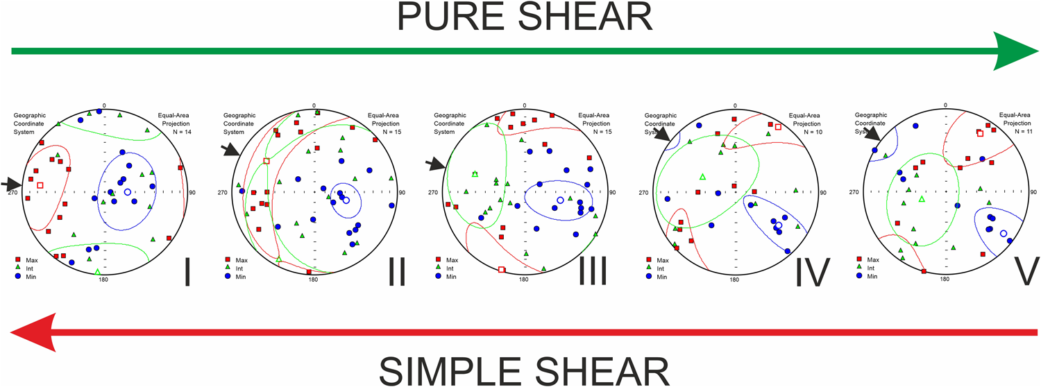
As noted earlier, there are three types of AMS projections in the studied locations (Fig. 5). In the first case, where L predominates, the k max axis is relatively well ordered, and the other axes of susceptibility are stretched around it (e.g., Kijaszkowo, site 2). In such a situation, the direction of ice-sheet movement was determined based on the orientation of the k max axis. This means that mineral/magnetic grains are arranged with their longest axis parallel to the movement of the ice sheet. The second type of magnetic fabrics concerns the situation in which F prevails in the tested fabrics. In this case, the k min axis is relatively well ordered, and the other axes lie in a plane perpendicular to this axis. The first subtype of foliated AMS is a situation in which the k max and k min axes lie in the direction of the ice-sheet movement (e.g., Karnkowo, site 17; Piątki, site 22). To sum up, in both situations described earlier, the direction of the ice-sheet movement can be determined on the basis of the orientation of the k max axis, despite the fact that the fabrics look different (T < 0 or T > 0). The mechanism responsible for such arrangement of mineral grains is simple shear (Shumway and Iverson, Reference Shumway and Iverson2009; Thomason and Iverson, Reference Thomason and Iverson2009; Fig. 10, I). The direction of shear strain is the result of the horizontal force associated with the movement of the ice sheet and the vertical force associated with the vertical pressure of the ice mass.
Types of magnetic fabrics (I–V) depending on the distribution of forces acting on the tested tills (squares, axis of maximum magnetic susceptibility; triangles, axis of intermediate magnetic susceptibility; circles, axis of minimum magnetic susceptibility; arrows, interpreted direction of ice-sheet movement).
During the laboratory work carried out by Hooyer et al. (Reference Hooyer, Iverson, Lagroix and Thomason2008), no correlation was found between the values of the shear forces acting on the till and the values of the T parameter. This indicates the lack of a direct relationship between the magnitude of simple shear and the type of magnetic fabric. The reason for this may be related to the type of minerals responsible for AMS. Magnetic fabrics with predominant L may be caused by magnetite grains, which are characterized by negative values of the T parameter, while foliation fabrics may be associated with the influence of paramagnetic minerals, including lamellar minerals, on anisotropy (see “Magnetization Carriers”).
Contrary to the value of parameter T, it was shown that the eigenvalues, S 1, are a good indicator of shear intensity. For fabrics included in the two cases described earlier, the value of S 1 for the k max axis ranges from 0.442 to 0.733, with an average of 0.585 (Fig. 5, Table 1). Based on research by Hooyer et al. (Reference Hooyer, Iverson, Lagroix and Thomason2008), it can be concluded that the S 1 values obtained indicate a small value of simple shear forces acting during the accumulation of the tested tills. The declining values of simple shear may be a reflection of the weakening dynamics of the ice sheet. The record of slight dynamics of the ice sheet may correlate with the 2 m depth of AMS till sampling. It seems quite possible that the tills of the subsurface layers are a record of a rather final stage of ice-sheet deposition. The degree of orientation of the magnetic susceptibility axis may also be influenced by the content of the gravel fraction in tills. For example, the highest value of the S 1 eigenvalue for the k max axis in the range of 0.654–0.733 is found in tills with the smallest gravel fraction content at the level of 0.32–0.65%. One of the lowest values of S 1 eigenvalue for the k max axis, in the range of 0.422–0.462, refers to tills with the highest gravel fraction content in the range of 2.77–3.63%. It is worth emphasizing, however, that the relationship does not show strong, direct correlations based on the results from all surveyed locations. Of course, it cannot be ruled out that postdepositional processes influenced the arrangement of grains in tills or the formation of new mineral facies, especially in areas with decalcified tills.
In addition to the declination of the k max axis, which is aligned with the direction of ice-sheet movement, its inclination is also characteristic. Based on laboratory studies (Hooyer et al. Reference Hooyer, Iverson, Lagroix and Thomason2008), it was found that under the action of simple shear, the k max axis is inclined at an angle of 16–25° toward the front of the ice sheet, provided the ice sheet was moving on a relatively flat surface, without much variation in the relief. In the studied tills, in individual sites, the average inclination of k max axis is 4–46° toward the ice-sheet front for some sites and 2–23° in the opposite direction for other sites. This means that only some of the sites (Kikoł, site 11; Karnkowo, site 17; Białowieżyn, site 18; Piątki, site 22; Zawidz Kościelny, site 31; Stara Biała, site 32) are characterized by a horizontally oriented shear plane, which proves that the ice sheet moved on a relatively flat surface. In the case of the remaining sites, the ice sheet moved along a substrate with a variable inclination (Shumway and Iverson, Reference Shumway and Iverson2009).
The second subtype of foliated fabrics are those AMS projections in which the k int and k min axes lie in the line of direction of ice-sheet movement (Fig. 5). In this case, the k max axis is oriented perpendicularly or almost perpendicularly to the interpreted direction of ice-sheet movement (e.g., Moszczonne, site 6; Chlebowo, site 13). Such arrangement of the magnetic susceptibility axis may be a record of the action of pure shear on the studied tills (Ankerstjerne et al., Reference Ankerstjerne, Iverson and Lagroix2015; Parés, Reference Parés2015; McCracken et al., Reference McCracken, Iverson, Benediktsson, Schomacker, Zoet, Johnson, Hooyer and Ingólfsson2016). Pure shear may have acted during the deposition of tills along with simple shear or influenced by glacitectonic deformations on already deposited sediment. As a result of the action of pure shear, the k min axis aligns with the action of the highest stresses acting on the sediment, while the k max axis aligns with the direction of greatest stretching in the deformed tills (Fig. 10, V).
To sum up, in the studied tills, the arrangement of mineral grains in extreme cases was influenced by: (1) simple shear (Fig. 10, I) combined with subglacial deformations, the basic mechanism associated with the movement of the ice sheet, or (2) pure shear (V) associated with glacitectonic deformations of the deposited sediment. Intermediate states have also been preserved in the tills, that is, a record of two types of shearing (II–IV). Most likely, in this case, the tills were initially deposited by simple shear, and then, as a result of postdepositional glaciotectonic processes of varying intensity, the mineral grains were reoriented. It is also worth emphasizing that in the first phases of deformation, only grain reorientation may occur without visible deformation structures.
Directions of ice-sheet movement on the basis of AMS and orientation of glacial landforms on the DEM
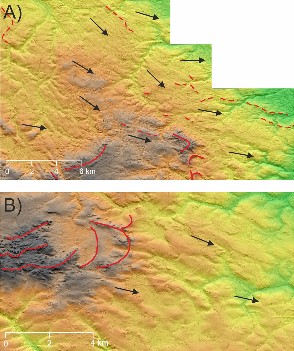
The results obtained from the AMS method indicate that in the northern part of the Płońsk Plateau, the ice sheet moved from north to south (Nowe Piastowo, site 28; Zawidz Kościelny, site 31), while in the central part of the area, there was a change of direction to WNW-ESE (Rychacice, site 30) or W-E (Kuchary-Jeżewo, site 33) (Figs. 4 and 5). Similar data are also provided by the analysis of the DEM. In the eastern part of the plateau, a network of glacial morpholineaments was identified (Fig. 11). The first of them is located near Drobin. These are extremely elongated depressions of a small depth (up to about 1 m) and strongly elongated hillocks up to about 1 m high (Fig. 11A). In the study area, they stretch for a distance of about 27 km. Their orientation changes from NW-SE in the north to WNW-ESE in the south. Remains of these forms were also located north of Bielsk (orientation WNW-ESE or WE) and northwest of Bielsk (orientation NW-SE). These forms can be classified as megascale glacial lineations (MGLs) (e.g., Newton and Huuse, Reference Newton and Huuse2017) on the basis of which it is possible to determine the direction of ice-sheet movement, which in this case is parallel to their course, that is, NW-SE and WNW-ESE. MGLs also appear to occur in moraines located to the northeast of the study area (Fig. 11A, dashed lines), which proves that the ice sheet crossed these moraines. The moraines near Staroźreby stand in opposition (Fig. 11A and B, solid lines), which are higher, better preserved, and accumulated on MGLs. This proves that the moraines near Staroźreby are younger than those located southeast of Drobin. In the eastern part of the Płońsk Plateau, there are also visible elements of the surface shape indicating the transformation of the previously formed relief by the ice sheet (Fig. 11B). These forms are characterized by an elongated, often streamlined shape and orientation along the WNW-ESE or NW-SE line, indicating the direction of ice-sheet movement.
(A) An example of the formation of megascale glacial lineations; (B) relief transformed by the activity of the ice sheet (red lines: solid, sequences of terminal moraines from the Saalian glaciation; dashed, sequences of overridden moraines; arrows, interpreted direction of ice-sheet movement during the Saalian glaciation); location of the outlined area in Fig. 4.
In the Urszulewo Plain and the western part of the Płońsk Plateau occupied by the ice sheet during the Weichselian glaciation, the reconstructed directions of ice-sheet movement assume a radial character, typical of the frontal parts of the glacial lobe (Figs. 4 and 5). In the northern part of the described area, north of Tłuchowo, the ice sheet generally moved from SW to NE. This direction is confirmed by the AMS data from the Łąkie (site 15) and the arrangement of glacial meltwater channels and terminal moraines in this region. Between Tłuchowo and Rembelin, the ice sheet moved along a line similar to W-E or WNW-ESE, which is indicated by the arrangement of glacial channel valleys, moraine strings, and AMS data from the Kamień Kotowy (site 27). In the frontal part of the ice sheet, there was a local change in the direction of movement of the ice sheet to NW-SE, which is confirmed by data from the Rempin (site 29; Figs. 4 and 5). In the vicinity of the Vistula valley, between Rembelin and Płock, the ice sheet moved along the NW-SE or WNW-ESE line, parallel to the axis of the Vistula valley. The WSW-ENE direction interpreted in the Stara Biała (site 32) was also recorded in this area. The radial distribution of the ice-sheet movement directions is confirmed by the orientation of the moraine hills in this area (Fig. 4). Also, Skompski (Reference Skompski1969) presented similar conclusions based on till clast fabric measurements in available exposures, stating that between Rembelin and Płock the ice sheet moved along the NW-SE line in the immediate vicinity of the Vistula valley, while in the area north of Płock, the direction of ice-sheet movement was from SW to NE or from WSW to ENE.
In the area of the Dobrzyń Lakeland, the directions of ice-sheet movement interpreted on the basis of AMS were compared with the directions obtained on the basis of the analysis of the DEM (Teodorski, Reference Teodorski2023). The orientation of the “minor end moraines” and crevasse forms on the DEM indicates that the ice sheet moved from NW to SE between Dobrzyń and Rembelin. AMS data from the Dobrzyń (site 35) confirm this direction of movement of the ice sheet (Figs. 4 and 5). On the other hand, the measurements of clast fabric in till exposures located to the east of Dobrzyń (Skompski, Reference Skompski1969) may indicate local changes in the direction of ice-sheet movement toward more SW-NE or WSW-ESE in the frontal parts of the ice sheet. However, it is currently difficult to reconcile the results of clast fabric measurements with the postulated minor end moraines in the area discussed (Teodorski, Reference Teodorski2023), which indicate the direction of ice-sheet movement from NW to SE. In the northern part of this area, in the Michałkowo (site 26), a W-E direction was interpreted. Despite the low strength of the magnetic fabric in this site (S 1 < 0.6), this direction is still correct in the context of the arrangement of terminal moraine sequences. At the Mokowo (site 25), the direction of movement on the SSW-NNE line was determined on the basis of the AMS method, that is, almost perpendicular to the one interpreted on the basis of the minor end moraines and crevasse form orientations on the DEM. It is difficult to explain such a direction of movement of the ice sheet. Perhaps the magnetic fabric from this site represents the arrangement of mineral grains in minor end moraines located mainly to the west of this site (Fig. 4, thin red line). The Wierznica (site 24) is between two strings of minor end moraines. The direction of ice-sheet movement interpreted on the basis of the AMS method is WSW-ENE and is consistent with the direction of movement determined on the basis of the orientation of minor end moraines. The next AMS site in the southern part of the Dobrzyń Lakeland is located in Włocławek (site 34). The mean direction of ice-sheet movement determined on the basis of the AMS method is SW-NE. On the basis of the crevasse forms and meltwater channel orientation on the DEM model, the perpendicular direction, NW-SE, was interpreted, that is, in line with the mean orientation of k max axis. Looking at the magnetic fabric in detail from this site, in the orientation of the k max axis, the component with the N-S orientation is clearly visible. Probably two directions of movement of the ice sheet, NW-SE and S-N, were recorded in the vicinity of the studied site, which resulted in a mean direction of movement from SW to NE. At the Nowa Wieś (site 21), both methods indicate the direction of movement on the NW-SE line.
In the central part of the Dobrzyń Lakeland, the orientation analysis of the terminal moraines, minor end moraines, crevasse forms, eskers, and meltwater channels on the DEM showed a change in the direction of the ice-sheet movement from NW-SE or NNW-SSE in the north to WNW-ESE toward the south. Based on the AMS method, similar conclusions can be drawn (Figs. 4 and 5). The sites located in the north of the region indicate the direction of movement NW-SE (Makowiska, site 10), NNW-SSE (Janowo, site 12), or N-S (Chlebowo, site 13). The sites in the more southern part are characterized by a more latitudinal direction of movement, along the lines WSW-ENE (Białowieżyn, site 18), W-E (Złotopole, site 14; Karnkowo, site 17; Głodowo, site 19; Ignackowo, site 20; Piątki, site 22), and WNW-ESE (Głogi, site 16). Only at the Bałdowo (site 23) is the direction of movement N-S.
In the northern part of the Dobrzyń Lakeland, in the western glacial lobe, based on the orientation of the terminal moraines, minor end moraines, crevasse forms, and meltwater channels on the DEM, it was found that the ice sheet moved from NW-SE in the north to N-S in the south. The AMS data indicate the direction of the ice-sheet movement to N-S (Mazowsze, site 1; Kijaszkowo, site 2). These results correspond with the course of the main glacial channel valley in this area, which proves that the direction of the N-S movement is characteristic of this part of the lobe (Figs. 4 and 5). However, in the northwestern part of the lobe, the NW-SE direction is correct, as evidenced by the orientation of crevasse forms, glacial channel valleys, and moraine hills. In the southern part of the lobe, AMS data indicate radiating directions of ice-sheet movement (Figs. 4 and 5). At the sites of Steklin (site 7) and Wawrzonkowo (site 8), the direction ENE-WSW was recorded; at Sumin (site 9), N-S; and at Moszczonne (site 6) and Kikoł (site 11), WNW-ESE and W-E. Based on the DEM analysis, a series of minor end moraines were determined in this area (Teodorski, Reference Teodorski2023), but their general latitudinal orientation indicates the direct direction of the N-S movement. This may indicate that minor end moraines were formed at a different time than the deposition of glacial tills, which is confirmed by studies carried out in the United States (e.g., Cline et al., Reference Cline, Iverson and Harding2015). On the other hand, the forms interpreted as minor end moraines may actually represent crevasse forms that are parallel to the direction of ice flow interpreted based on AMS samples at sites 7 and 8. In the second central glacial lobe, whose maximum extent is determined by moraines near Chrostkowo, the direction of ice-sheet movement along the NNW-SSE and NW-SE lines in the eastern part of this lobe was interpreted on the basis of the terminal moraines, minor end moraines, and meltwater channel orientations on the DEM. There are two sites within the described glacial lobe, in Nowa Wieś (site 4) and Wildno (site 5). AMS data from both sites point to the NW-SE direction in the southern part of this lobe. The NNW-SSE ice flow direction is similar to that which can be obtained based on the till fabric measured in the subglacial till building glacial curvilineation located in the vicinity of Wielgie (Lesemann et al., Reference Lesemann, Piotrowski and Wysota2014). The differences between the two methods may result from the fact that in this area, there are no significant areas occupied by glacial plateaus, which makes it difficult to analyze the directions of ice-sheet movement in detail based on the DEM. It seems reasonable to assume that the ice sheet in this glacial lobe, at least in its southern part, moved from NW to SE. New data were also brought by the AMS data from the Klonowo (site 3), which indicate the NNE-SSW direction of movement in the western part of the lobe.
To sum up, the AMS method, in many cases, provides similar information to that obtained from the analysis of the DEM. It also allows the directions of ice-sheet movement to be specified in areas where the glacial relief is not sufficiently developed.
Paleoenvironmental reconstruction of the study area
The study area was eventually covered by an ice sheet during two different glaciations. Most of the Płońsk Plateau was covered for the last time by the ice sheet of the Saalian glaciation. The oldest extent of the ice sheet in the study area is marked by moraines near Bodzanów and northeast of Wyszogród (stage 1; Fig. 12). The latter moraines are well developed and clearly visible on the DEM model. These moraines were formed during one of the recessive phases of the glaciation. The next stage of recession is the stagnation of the ice-sheet front on the line of moraines near Drobin (stage 2; Fig. 12). In the study area, there are hardly find any landforms other than moraines, from which it is possible to determine the directions of ice-sheet movement during these two stages. Only on the basis of the orientation of the moraines can it be concluded that the ice sheet moved along a line similar to N-S. The next stage is related to the re-advance of the Saalian glaciation ice sheet. In the northern part of the research area (east of Sierpc), the ice sheet moved from north to south, and then between Drobin and Radzanowo changed its direction to WNW-ESE. The maximum extent of this transgression should be sought east of the study area. During the advance, the ice sheet crossed the moraines near Drobin from the older phase of this glaciation. The occurrence of MGLs on the moraine forms of stage 2 speaks for a later time for this transgression in relation to the previous stages. During the next ice-sheet recession, moraines accumulated near Staroźreby, Radzanowo, and Mochcino (stage 3; Fig. 12). Moraines, in many cases, are well preserved, have a different orientation than those from earlier stages of the ice-sheet existence, and to the northeast of Staroźreby, they lie on MGLs. The next stage is marked by moraines south of Kurowo (stage 4; Fig. 12) and may be a record of a local transgression during the Saalian glaciation or the Weichselian glaciation, as indicated by Dzierżek (Reference Dzierżek2009).
Paleogeographic sketch showing the development and disappearance of the ice sheet of the Saalian and Weichselian glaciations in north-central Poland (colored lines: solid, lines of terminal moraines; dashed lines, lines of overridden moraines; 1–8, stages of the ice-sheet extent; arrows, interpreted direction of ice-sheet movement; LGM, maximum extent of the Weichselian glaciation ice sheet)
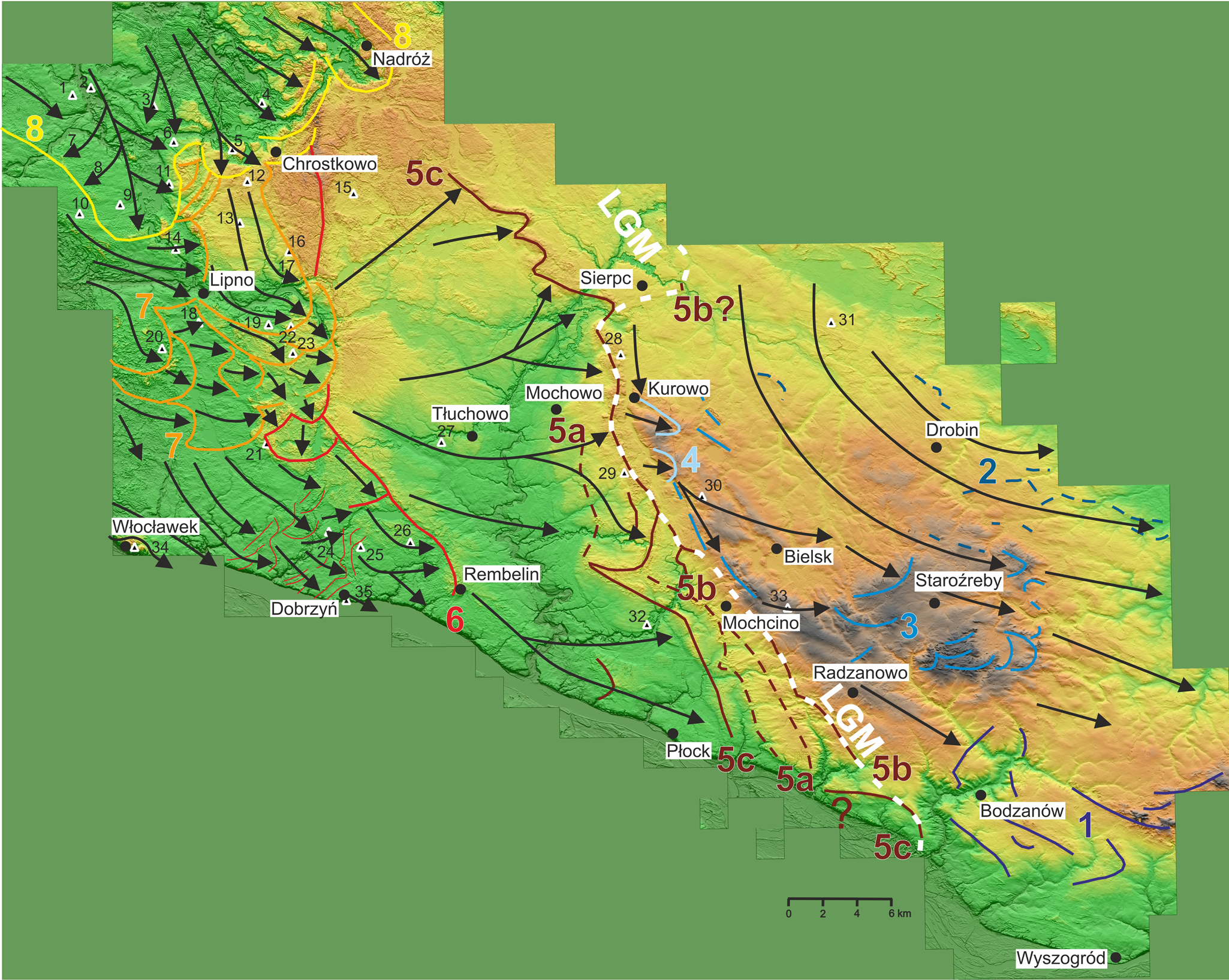
The next stages of the ice-sheet advance are related to the ice sheet of the Weichselian glaciation. In the area close to the local LGM, several sequences of terminal moraine forms were interpreted on the basis of the DEM. The first of them reflects the extent of the ice-sheet front before the local LGM (stage 5a; Fig. 12). Subsequently, transgression occurred, and the ice sheet crossed the previously deposited moraines from stage 5a. The existence of overridden moraines in this region is also indicated by Roman (Reference Roman2010). Moraine forms also occur to the northwest and southeast of Mochcino (stage 5b; Fig. 12). They determine the maximum extent of the ice sheet of the Weichselian glaciation in this area. The next stage of the ice-sheet front stillstand can be associated with the best-preserved and longest sequence of terminal moraines (stage 5c; Fig. 12). This sequence is particularly visible in the area north of the Mochowo–Kurowo line. It is debatable whether the sequence of terminal moraines described above can be a record of the local LGM in the northern part of the study area. According to Kotarbiński (Reference Kotarbiński1998), in this region, the extent of the ice sheet during the local LGM is determined to the east of Sierpc and is based on the location of the few preserved single terminal moraine hills. This position is also confirmed by Krupiński (Reference Krupiński2005), who points to two sites of interglacial sediments located north of Sierpc, where sediments belonging to the Eemian interglaciation are covered with glacial till (or its residue) of the Weichselian glaciation. On the other hand, the local LGM line running west of Sierpc is indicated by Lamparski (Reference Lamparski and Dzierżek2001), and it coincides with the location of the described moraine sequence. Undoubtedly, the described series of moraines in its central part exceeds the local LGM moraines from stage 5b. It is possible that terminal moraines have also been preserved in the southern part of the study area, in the immediate vicinity of the Vistula valley, which would also be a record of this stage of the ice-sheet extent. Possibly occurring moraines may also overprint the moraines from stage 5b. This information suggests that the LGM in north-central Poland is asynchronous. Based on the this, it can be concluded that in the period around the local LGM, there were several oscillations of the ice-sheet front. At that time, the ice sheet was characterized by directions of movement from SW-NE in the north to NW-SE in the south. Due to the accumulation of fluvioglacial sediments on the Urszulewo Plain, there are no terminal moraines that could mark the subsequent stages of ice-sheet recession. In the vicinity of the Vistula valley, between Rembelin and Płock, remains of moraines were interpreted, which Roman (Reference Roman2010) interprets as overridden moraines (Fig. 12).
In the Dobrzyń Lakeland, the period of ice-sheet recession can be divided into three stages, described in detail in Teodorski (Reference Teodorski2023). In the first stage, the easternmost front of the ice sheet stopped in the vicinity of Rembelin (stage 6; Fig. 12). Dzierżek (Reference Dzierżek2009) also presents a similar assumption. On the other hand, Roman (Reference Roman2010, Reference Roman2019) does not describe any terminal moraines in this area, indicating a uniform advance and recession of the ice sheet. Then, the ice sheet gradually retreated from the lakeland. The short-term advance of the ice-sheet front is indicated by minor end moraines between Włocławek (site 34) and Dobrzyń (site 35). The directions of ice-sheet movement generally change from similar to N-S in the north through NW-SE to W-E or locally SSW-NNE in the southeastern part. The next stage (stage 7; Fig. 12) is associated with the transgression of a small ice stream in the central part of the Dobrzyń Lakeland. During this stage, the ice sheet crossed the oldest moraines located in the eastern part of the Dobrzyń Lakeland and the ice sheet generally moved WNW-ESE. The last stage of the ice-sheet extent in the Lakeland (stage 8; Fig. 12) is associated with the transgressive–regressive Kujawy–Dobrzyń subphase (Lamparski Reference Lamparski and Kostrzewski1991; Niewiarowski et al., Reference Niewiarowski, Olszewski and Wysota1995; Dzierżek, Reference Dzierżek2009). The ice-sheet front stopped on the line of moraines near Nadróż and Chrostkowo during the last stage of deglaciation. During this subphase, the ice sheet generally moved along the NNW-SSE line. Dzierżek (Reference Dzierżek2009) also determined a similar direction of ice flow based on the orientation of moraine ridges in the northern part of the lakeland. The directions of ice flow obtained in the Dobrzyń Lakeland area generally agree with those obtained by Morawski (Reference Morawski2009).
Conclusions
Based on the conducted research, several new conclusions can be drawn about the ice-sheet dynamics in the area of north-central Poland during the Saalian and Weichselian glaciations.
On the basis of the AMS method, it was found that there are magnetic fabrics in the tested tills whose arrangement is due to simple shear, pure shear, or a mixture of the two types. Simple shear is associated with subglacial deformations in the bed of the ice sheet. Pure shear occurs during syn- or postdepositional glacitectonic processes.
The arrangement of mineral grains in the examined tills indicates generally low values of simple shear acting during their deposition, which may be a reflection of the weakening subglacial deformations and the decreasing dynamics of the ice sheet. Glaciotectonic processes associated with the action of pure shear indicate a temporary, local increase in ice-sheet activity.
The directions of ice-sheet movement determined on the basis of the AMS method are consistent with the directions of movement interpreted on the basis of the DEM model. This shows that the AMS method can be used for reconstructing regional pattern of the ice flow direction and can yield new data on the Pleistocene glaciations.
The innovative method of sampling glacial tills from under the surface of the plateau turned out to be effective and has a chance to contribute to even greater dissemination of the use of the AMS method in Quaternary studies concerning the determination of ice-sheet movement and reconstructing processes of subglacial till formation.
The composition of the magnetic minerals in tills depends on their age. Magnetite, hematite, titanomagnetite, and/or maghemite have been identified in the tills of the Weichselian glaciation. Tills from the Saalian glaciation contain mainly magnetite and hematite. At least in some cases of the examined tills, paramagnetic minerals, such as some clay minerals or minerals from the mica group, are responsible for AMS.
During the analysis of the DEM, previously unidentified landforms in north-central Poland were determined. Megascale glacial lineations were discovered in the Płońsk Plateau. In the area of the local LGM, several sequences of terminal moraine forms, previously not described or only fragmentarily described in this part of Poland, were located.
In the area of the Płońsk Plateau, in the generally recessive phase of the Saalian glaciation, the transgression of the ice sheet was interpreted. The ice sheet in the northern part of the Plateau area moved along the N-S line, and then in the central part it changed direction to WNW-ESE. The direction of movement close to latitudinal is perpendicular to the main direction of movement during the recession of the ice sheet of the Saalian glaciation, which indicates a certain distinctiveness of this transgressive glacial stage.
Within the area occupied by the Weichselian ice sheet, four glacial episodes with separate directions of ice-sheet movement can be distinguished: (1) the stage of the maximum extent of the ice sheet; (2) the stillstand of the ice sheet front in the vicinity of Rembelin; (3) the stage of ice-sheet readvance in the central part of the Dobrzyń Lakeland; and (4) the stage of the Kujawy–Dobrzyń subphase.
Acknowledgments
The author is grateful to Michał Bakiera for help with fieldwork. The author would like to thank Sebastian Richiano and an anonymous reviewer for all the comments and suggestions that improved the article. This research did not receive any specific grant from funding agencies in the public, commercial, or not-for-profit sectors.



