2 Numerical simulations

Simulations were performed with the NLS equation and the MNLS equation of Dysthe (Reference Dysthe1979). These employ an expression for surface elevation on the form

where $\text{i}=\sqrt{-1}$ is the imaginary unit, c.c. denotes complex conjugate and $B$ is the first harmonic complex amplitude of the waves. We let the phase function be $\unicode[STIX]{x1D712}=(\boldsymbol{k}_{p}\boldsymbol{\cdot }\boldsymbol{x}-\unicode[STIX]{x1D714}_{p}t)$ where $\boldsymbol{x}=(x,y)$ is the horizontal position vector, $t$ is time, $\boldsymbol{k}_{p}=(k_{p},0)$ is the peak wave vector and $\unicode[STIX]{x1D714}_{p}=\unicode[STIX]{x1D6FA}(\boldsymbol{k}_{p})=(g|\boldsymbol{k}_{p}|)^{1/2}$ is the LDR peak frequency.

The zeroth harmonic, $\bar{\unicode[STIX]{x1D702}}$ , and the complex amplitudes of the higher harmonics, $B_{2},B_{3},\ldots ,$ can be expressed in terms of $B$ , see Toffoli et al. (Reference Toffoli, Gramstad, Trulsen, Monbaliu, Bitner-Gregersen and Onorato2010) equation (3.4). We shall only be concerned about the spectral contribution of $\unicode[STIX]{x1D702}$ close to the peak $k_{p}$ and $\unicode[STIX]{x1D714}_{p}$ . For this reason we only consider the contribution from $B$ for reconstruction of the surface elevation in (2.1).

The MNLS equation is

where $\ast$ denotes complex conjugate.

The induced mean flow $\bar{\unicode[STIX]{x1D719}}$ is governed by

where $\unicode[STIX]{x1D735}=(\unicode[STIX]{x2202}/\unicode[STIX]{x2202}x,\unicode[STIX]{x2202}/\unicode[STIX]{x2202}y,\unicode[STIX]{x2202}/\unicode[STIX]{x2202}z)$ .

The differential operator ${\mathcal{L}}$ accounts for linear dispersion. Following Trulsen et al. (Reference Trulsen, Kliakhandler, Dysthe and Velarde2000) it can be written in exact form

By considering the first three terms of (2.2) the NLS equation is recovered.

Most of the simulations are initialized with a Gaussian wave vector spectrum

symmetric around the peak wave vector $\boldsymbol{k}_{p}=(k_{p},0)$ where $\boldsymbol{k}=(k_{x},k_{y})$ is the horizontal wave vector and $\unicode[STIX]{x1D70E}_{x}$ and $\unicode[STIX]{x1D70E}_{y}$ are non-dimensional longitudinal and transversal bandwidths, respectively. The characteristic amplitude of the surface elevation $\unicode[STIX]{x1D702}$ is $a_{c}=(2\langle \unicode[STIX]{x1D702}^{2}\rangle )^{1/2}$ where $\langle \cdot \rangle$ denotes statistical averaging. The spectrum fulfils the normalization criterion

The average steepness is $\unicode[STIX]{x1D716}=a_{c}k_{p}$ . We perform simulations with $\unicode[STIX]{x1D716}=$ 0.04, 0.06, 0.08 and 0.10. The highest steepness $\unicode[STIX]{x1D716}=0.10$ corresponds to the average maximum steepness observed in the ocean as demonstrated by figure 2 in Socquet-Juglard et al. (Reference Socquet-Juglard, Dysthe, Trulsen, Krogstad and Liu2005).

For comparison with the MARIN laboratory data we perform simulations initialized with a Joint North Sea Wave Project (JONSWAP) spectrum (Hasselmann et al. Reference Hasselmann, Barnett, Bouws, Carlson, Cartwright, Enke, Ewing, Gienapp, Hasselmann and Kruseman1973),

with Phillips factor $\unicode[STIX]{x1D6FC}$ , peak enhancement factor $\unicode[STIX]{x1D6FE}=3.3$ and

The directional spreading used for initialization was

where $\unicode[STIX]{x1D6E4}$ is the gamma function, $N$ is a spreading parameter and $\unicode[STIX]{x1D703}$ is the direction. Simanesew et al. (Reference Simanesew, Krogstad, Trulsen and Nieto Borge2016) showed that this initially frequency-independent directional spreading evolved into a frequency-dependent directional spreading when simulated with the MNLS equation.

For initialization of simulations the spectrum (2.9) is transformed to a wave vector spectrum

where $\boldsymbol{k}=(k\cos \unicode[STIX]{x1D703},k\sin \unicode[STIX]{x1D703})$ and $\unicode[STIX]{x1D714}=\unicode[STIX]{x1D6FA}(\boldsymbol{k})$ according to the LDR.

To solve the model equations numerically we use the method described by Lo & Mei (Reference Lo and Mei1985, Reference Lo and Mei1987) with periodic boundary conditions in both horizontal directions. In order to employ the narrow-banded models we truncate the spectra within $|\boldsymbol{k}-\boldsymbol{k}_{p}|\leqslant k_{p}$ around the peak $\boldsymbol{k}_{p}$ . We let $x$ and $y$ be the longitudinal and transversal coordinates, respectively. The computational domain extends over 70 peak wavelengths $\unicode[STIX]{x1D706}_{p}$ in both the $x$ and $y$ -directions. For directional waves we use a uniform grid of $N_{x}\times N_{y}=512\times 512$ nodes. For unidirectional waves we use a uniform grid of $N_{x}=512$ nodes along the $x$ -axis. In time we let the waves evolve for 150 peak periods $T_{p}$ .

We perform a number of unidirectional and directional simulations with the Gaussian spectrum (2.7) for steepnesses $\unicode[STIX]{x1D716}=$ 0.04, 0.06, 0.08 and 0.10. For all steepnesses we perform simulations for longitudinal bandwidth $\unicode[STIX]{x1D70E}_{x}$ between 0.07 and 0.49 and transversal bandwidth $\unicode[STIX]{x1D70E}_{y}$ between 0 and 0.50, in steps of 0.02. The number of simulations is $4\times 22\times 26=2288$ . In addition we perform 3 simulations with the JONSWAP spectrum (2.9)–(2.12) for comparison with the MARIN laboratory data.

From surface elevations $\unicode[STIX]{x1D702}(x,y,t)$ , the $(k_{x},k_{y},\unicode[STIX]{x1D714})$ -spectra are obtained by discrete Fourier transform. In the following we present $(k,\unicode[STIX]{x1D714})$ -spectra obtained by transforming $(k_{x},k_{y},\unicode[STIX]{x1D714})$ -spectra from Cartesian to polar coordinates using the relations $k_{x}=k\cos \unicode[STIX]{x1D703}$ and $k_{y}=k\sin \unicode[STIX]{x1D703}$ and by integrating over $\unicode[STIX]{x1D703}$ .

To describe deviation between dispersion of simulated waves and LDR we propose the following deviation parameter

In (2.13), $\unicode[STIX]{x1D6FA}(k)$ is given by (1.1), $S_{1}$ is the $(k,\unicode[STIX]{x1D714})$ -spectrum from the simulations and $\unicode[STIX]{x1D714}_{p}$ is the peak frequency of the initial spectrum (2.7). The integrals are evaluated over the spectral domain within $|\boldsymbol{k}-\boldsymbol{k}_{p}|\leqslant k_{p}$ . Equation (2.13) can be regarded as a normalized first moment of deviation from LDR.

For comparison of simulated waves with LDR we compute the root mean square (RMS) wavenumber

corresponding to each frequency $\unicode[STIX]{x1D714}$ where $k=(k_{x}^{2}+k_{y}^{2})^{1/2}$ and $S_{2}$ is the $(k_{x},k_{y},\unicode[STIX]{x1D714})$ -spectrum from the simulations.

The bandwidths $\unicode[STIX]{x0394}\unicode[STIX]{x1D714}$ and $\unicode[STIX]{x0394}k_{y}$ used for BFI (1.2) and $L_{c}$ (1.3), respectively, were determined from the initial spectrum (2.7) using half-width at half-peak (HWHP). The bandwidth $\unicode[STIX]{x0394}\unicode[STIX]{x1D714}$ was found by rewriting (2.7) to a $k$ -spectrum using polar coordinates and $\unicode[STIX]{x0394}\unicode[STIX]{x1D714}$ was computed from $\unicode[STIX]{x0394}\unicode[STIX]{x1D714}=\unicode[STIX]{x1D714}_{p}((1+\unicode[STIX]{x0394}k/k_{p})^{1/2}-1)$ where $\unicode[STIX]{x0394}k$ is HWHP of the $k$ -spectrum. The bandwidth $\unicode[STIX]{x0394}k_{y}$ was computed from HWHP of the $k_{y}$ -spectrum corresponding to (2.7).

While $\unicode[STIX]{x0394}k_{y}$ depends on $\unicode[STIX]{x1D70E}_{y}$ only, $\unicode[STIX]{x0394}\unicode[STIX]{x1D714}$ depends on both $\unicode[STIX]{x1D70E}_{x}$ and $\unicode[STIX]{x1D70E}_{y}$ . As a consequence the data of BFI and $L_{c}$ are non-uniformly distributed given a uniform grid for $\unicode[STIX]{x1D70E}_{x}$ and $\unicode[STIX]{x1D70E}_{y}$ . In the following we present the scalar field of $\unicode[STIX]{x1D6FF}$ (2.13) as a function of BFI and inverse crest length $L_{c}^{-1}$ . In order to plot $\unicode[STIX]{x1D6FF}(\text{BFI},L_{c}^{-1})$ the scalar field is fitted to a uniform grid by cubic interpolation. As a consequence of the grid the upper right corners of the contour plots of $\unicode[STIX]{x1D6FF}$ are empty, see figure 5.

For the highest steepness $\unicode[STIX]{x1D716}=0.10$ , BFI ranges from 0.39 to 2.63. For the lowest steepness $\unicode[STIX]{x1D716}=0.04$ , BFI ranges from 0.15 to 1.05. For $\unicode[STIX]{x1D70E}_{y}$ between 0 and 0.50, $L_{c}$ ranges from 1.70 $\unicode[STIX]{x1D706}_{p}$ up to unidirectional waves. Correspondingly, $L_{c}^{-1}$ ranges from 0 to 0.59.

There have been recent attempts to combine BFI and directionality into a single directional BFI (Waseda, Kinoshita & Tamura Reference Waseda, Kinoshita and Tamura2009; Mori, Onorato & Janssen Reference Mori, Onorato and Janssen2011; Xiao et al. Reference Xiao, Liu, Wu and Yue2013) with the purpose of parameterizing kurtosis and rogue wave occurrence. Our purpose is different, to parameterize the deviation from the LDR, however, by comparing our results of $\unicode[STIX]{x1D6FF}$ to the directional BFI of Mori et al. (Reference Mori, Onorato and Janssen2011) we find that it could be a suitable parameter for identifying the deviation.

3 Numerical results

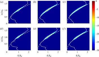
Figure 1 shows $(k,\,\unicode[STIX]{x1D714})$ -spectra from directional simulations with the highest steepness $\unicode[STIX]{x1D716}=0.10$ and the narrowest initial bandwidths $\unicode[STIX]{x1D70E}_{x}=0.07$ and $\unicode[STIX]{x1D70E}_{y}=0.02$ . Colours show spectral energy density in decibel (dB) relative to the peak. White dashed curves show LDR, $\unicode[STIX]{x1D6FA}(k)$ , from (1.1). Figures 1(a–c) and 1(d–f) show spectral evolution with regard to the NLS and MNLS equations, respectively. Figure 1(a,d) shows the $(k,\unicode[STIX]{x1D714})$ -spectra during the first fifty peak periods $t/T_{p}\in [0,50]$ , (b,e) shows $t/T_{p}\in [50,100]$ and (c,f) shows $t/T_{p}\in [100,150]$ .

Figure 1.

Evolution of $(k,\unicode[STIX]{x1D714})$ -spectra of directional wave field with $\unicode[STIX]{x1D716}=0.10$ and $\unicode[STIX]{x1D70E}_{x}=0.07$ and $\unicode[STIX]{x1D70E}_{y}=0.02$ . Colours: spectral energy density in dB. White dashed curves: LDR $\unicode[STIX]{x1D6FA}(k)$ from (1.1). White dotted curves: RMS wavenumber $k_{RMS}(\unicode[STIX]{x1D714})$ from (2.14). (a,d)  $t/T_{p}\in [0,50]$ ; (b,e)  $t/T_{p}\in [50,100]$ and (c,f)  $t/T_{p}\in [100,150]$ . (a–c) NLS equation. (d–f) MNLS equation.

Figure 1 shows the qualitative difference between spectral evolution for the NLS and MNLS equations. For the NLS equation, the spectral energy density grows symmetrically around the peak while for the MNLS equation it grows asymmetrically to wavenumbers and frequencies above peak.

Within $t/T_{p}\in [0,50]$ the waves quickly evolve into a state where spectral energy density deviates from the LDR. The white dotted curves show the RMS wavenumber, $k_{RMS}(\unicode[STIX]{x1D714})$ from (2.14), which confirms the deviation. For the NLS equation the deviation is pronounced both above and below peak while for the MNLS equation the deviation is pronounced only above peak. Above peak the MNLS equation contributes to a more pronounced deviation than the NLS equation during the time considered. Within $t/T_{p}\in [100,150]$ the spectral energy density is spread out to a rather broad distribution and starts to relax toward the LDR.

We performed simulations over longer times up to $200T_{p}$ which revealed that the directional waves eventually reach a quasi-stationary state with relaxation toward the LDR. Our narrow-banded unidirectional waves show deviation during the entire time up to $200T_{p}$ . The unidirectional waves do not reach a quasi-stationary state with relaxation toward the LDR. Thus a qualitative difference between directional and unidirectional wave propagation is observed. Qualitative difference was also observed by Gramstad & Trulsen (Reference Gramstad and Trulsen2007).

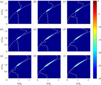
Figure 2 shows spectral evolution from directional simulations of the MNLS equation for steepnesses $\unicode[STIX]{x1D716}=$ 0.04, 0.06 and 0.08 and the narrowest initial bandwidths. Figures 2(a–c), 2(d–f) and 2(g–i) show spectral evolution for $\unicode[STIX]{x1D716}=0.04$ , 0.06 and 0.08, respectively. The waves evolve on Benjamin–Feir (BF) time scale $(\unicode[STIX]{x1D716}^{2}\unicode[STIX]{x1D714}_{p})^{-1}$ thus for different $\unicode[STIX]{x1D716}$ ranging from 0.04 to 0.10 characteristic time scales differ by approximately one order of magnitude. For $\unicode[STIX]{x1D716}=$ 0.04, 0.06, 0.08 and 0.10, BF time scale covers 100, 44, 25 and $16T_{p}$ , respectively. Figure 2 and figure 1(d–f) show that the occurrence of deviation depends on the characteristic time scales. For waves with high steepness deviation occurs, and relaxes toward LDR, sooner than for waves with lower steepness.

Figure 2.

Evolution of $(k,\unicode[STIX]{x1D714})$ -spectra of directional wave fields simulated using the MNLS equation with different $\unicode[STIX]{x1D716}$ and $\unicode[STIX]{x1D70E}_{x}=0.07$ and $\unicode[STIX]{x1D70E}_{y}=0.02$ . Colours: spectral energy density in dB. White dashed curves: LDR $\unicode[STIX]{x1D6FA}(k)$ from (1.1). White dotted curves: RMS wavenumber $k_{RMS}(\unicode[STIX]{x1D714})$ from (2.14). (a,d,g)  $t/T_{p}\in [0,50]$ ; (b,e,h)  $t/T_{p}\in [50,100]$ and (c,f,i)  $t/T_{p}\in [100,150]$ . (a–c)  $\unicode[STIX]{x1D716}=0.04$ ; (d–f)  $\unicode[STIX]{x1D716}=0.06$ and (g–i)  $\unicode[STIX]{x1D716}=0.08$ .

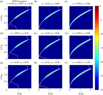
Figure 3 shows a selection of $(k,\unicode[STIX]{x1D714})$ -spectra of directional waves simulated with the MNLS equation with $\unicode[STIX]{x1D716}=0.10$ and different combinations of initial bandwidths $\unicode[STIX]{x1D70E}_{x}$ and $\unicode[STIX]{x1D70E}_{y}$ given in the titles of the panels. The spectral estimates are taken from $t/T_{p}\in [100,150]$ to observe occurrence of deviation farthest from initialization. Figure 3(a) is identical to figure 1(f). Figure 3(a,d,g) corresponds to $\unicode[STIX]{x1D70E}_{x}=0.07$ , (b,e,h) $\unicode[STIX]{x1D70E}_{x}=0.23$ and (c,f,i) $\unicode[STIX]{x1D70E}_{x}=0.49$ . Figure 3(a–c) corresponds to $\unicode[STIX]{x1D70E}_{y}=0.02$ , (d–f) $\unicode[STIX]{x1D70E}_{y}=0.26$ and (g–i) $\unicode[STIX]{x1D70E}_{y}=0.50$ .

Figure 3.

$(k,\unicode[STIX]{x1D714})$ -spectra of directional wave fields from time interval $t/T_{p}\in [100,150]$ simulated using the MNLS equation with $\unicode[STIX]{x1D716}=0.10$ and combinations of different $\unicode[STIX]{x1D70E}_{x}$ and $\unicode[STIX]{x1D70E}_{y}$ given in the title of the panels. Colours: spectral energy density in dB. Colour bar in dB. White dashed curves: LDR $\unicode[STIX]{x1D6FA}(k)$ from (1.1). White dotted curves: RMS wavenumber $k_{RMS}$ from (2.14).

From figure 3 it is observed that the occurrence of deviation depends on the initial bandwidths. For combinations of broad bandwidths corresponding to the four panels in the lower right corner of figure 3, deviation does not occur. To first order in magnitude, i.e. $\text{dB}>-10$ , and within the spectral radius of the simulations the spectral distribution resembles the shape of the LDR. Nevertheless, above peak the spectral distribution is shifted slightly toward wavenumbers and frequencies above LDR. This will be further explained below.

The simulations with $\unicode[STIX]{x1D716}=0.04$ , 0.06 and 0.08 show qualitatively similar results to those observed in figure 3 with occurrence of deviation for combinations of narrow bandwidths. For $\unicode[STIX]{x1D716}=$ 0.08 the shift above peak is observed for combinations of broad bandwidths similarly to that observed for $\unicode[STIX]{x1D716}=0.10$ while for $\unicode[STIX]{x1D716}=0.06$ and 0.04 the shift is less evident.

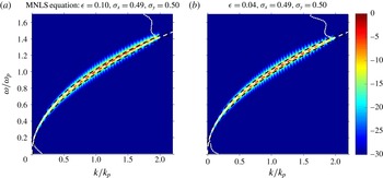
Figure 4 shows $(k,\unicode[STIX]{x1D714})$ -spectra of $\unicode[STIX]{x1D716}=0.10$ and 0.04 and broadest initial bandwidths $\unicode[STIX]{x1D70E}_{x}=0.49$ and $\unicode[STIX]{x1D70E}_{y}=0.50$ . Figure 4(a) corresponds to figure 3(i). For $\unicode[STIX]{x1D716}=0.10$ it is observed that the spectral distribution is shifted toward wavenumbers and frequencies above LDR. For $\unicode[STIX]{x1D716}=0.04$ the shift is less evident. The RMS wavenumber confirms the observation. Thus when the steepness is high, nonlinear evolution can cause a shift from the LDR for broad-banded waves. The black dashed curves show $\unicode[STIX]{x1D714}(k\pm \unicode[STIX]{x0394}k)\pm \unicode[STIX]{x0394}\unicode[STIX]{x1D714}$ as a function of $k$ where $\unicode[STIX]{x0394}k$ and $\unicode[STIX]{x0394}\unicode[STIX]{x1D714}$ are the resolutions along the wavenumber and frequency axes given by the discrete Fourier transform. These curves are commonly used as a criterion for the interpretation of marine radar images to filter out those spectral contributions that do not satisfy the LDR (Nieto Borge et al. Reference Nieto Borge, Rodríguez, Hessner and Izquierdo2004). For $\unicode[STIX]{x1D716}=0.10$ the spectral energy density is distributed along $\unicode[STIX]{x1D714}(k+\unicode[STIX]{x0394}k)+\unicode[STIX]{x0394}\unicode[STIX]{x1D714}$ above LDR while for $\unicode[STIX]{x1D716}=0.04$ the spectral energy density is distributed below $\unicode[STIX]{x1D714}(k+\unicode[STIX]{x0394}k)+\unicode[STIX]{x0394}\unicode[STIX]{x1D714}$ and closer to LDR.

Figure 4.

$(k,\unicode[STIX]{x1D714})$ -spectra of directional wave fields from time interval $t/T_{p}\in [100,150]$ simulated using the MNLS equation with $\unicode[STIX]{x1D716}=0.10$ and $\unicode[STIX]{x1D716}=0.04$ and combinations of the broadest bandwidths $\unicode[STIX]{x1D70E}_{x}$ and $\unicode[STIX]{x1D70E}_{y}$ given in the title of the panels. Colours: spectral energy density in dB. Colour bar in dB as in figure 3. White dashed curves: LDR $\unicode[STIX]{x1D6FA}(k)$ from (1.1). White dotted curves: RMS wavenumber $k_{RMS}$ from (2.14). Black dashed curves: radar filter $\unicode[STIX]{x1D714}(k\pm \unicode[STIX]{x0394}k)\pm \unicode[STIX]{x0394}\unicode[STIX]{x1D714}$ as a function of $k$ where $\unicode[STIX]{x0394}k$ and $\unicode[STIX]{x0394}\unicode[STIX]{x1D714}$ are the resolutions along the wavenumber and frequency axes given by the discrete Fourier transform.

Figure 5.

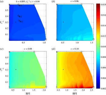
Colours: deviation parameter $\unicode[STIX]{x1D6FF}$ (2.13) as function of BFI and inverse crest length $L_{c}^{-1}$ for $\unicode[STIX]{x1D716}=0.04$ , 0.06, 0.08 and 0.10. Colour bar: magnitude of $\unicode[STIX]{x1D6FF}$ . Symbols showing location of data points corresponding to the initial bandwidths of the $(k,\unicode[STIX]{x1D714})$ -spectra shown in the diagonal panels of figure 3: ▫, $\unicode[STIX]{x1D70E}_{x}=0.07$ and $\unicode[STIX]{x1D70E}_{y}=0.02$ ; ♢, $\unicode[STIX]{x1D70E}_{x}=0.07$ and $\unicode[STIX]{x1D70E}_{y}=0.50;\times ,\unicode[STIX]{x1D70E}_{x}=0.49$ and $\unicode[STIX]{x1D70E}_{y}=0.02$ ; *, $\unicode[STIX]{x1D70E}_{x}=0.49$ and $\unicode[STIX]{x1D70E}_{y}=0.50$ and ●, $\unicode[STIX]{x1D70E}_{x}=0.23$ and $\unicode[STIX]{x1D70E}_{y}=0.26$ . Symbols showing location of data points corresponding to the BFI and inverse crest lengths $L_{c}^{-1}$ estimated from MARIN data: ▹, W1; ▵, W2; ◃, W3.

Figure 5 shows $\unicode[STIX]{x1D6FF}$ (2.13) as a function of BFI and $L_{c}^{-1}$ for 2288 simulations of the MNLS equation with $\unicode[STIX]{x1D716}=$ 0.04, 0.06, 0.08 and 0.10. The spectral estimates for $\unicode[STIX]{x1D6FF}$ are taken from $t/T_{p}\in [100,150]$ . Note that the BFI axes are different due to the different steepnesses involved. Symbols show the locations of spectra with bandwidths corresponding to diagonal panels of figure 3. Triangle symbols show the locations of data points corresponding to BFI and $L_{c}^{-1}$ estimated from the MARIN data and will be further explained in § 4.

For all steepnesses we find that the deviation from the LDR is most pronounced when the BFI is high and crests are long, and the deviation increases when the BFI increases. The highest magnitudes of $\unicode[STIX]{x1D6FF}$ were found for $\unicode[STIX]{x1D716}=$ 0.10. In particular, the highest magnitude for $\unicode[STIX]{x1D6FF}$ was found for the highest BFI given for unidirectional waves with $\unicode[STIX]{x1D716}=$ 0.10. For $\unicode[STIX]{x1D716}=0.10$ there is a sharp transition between high and low magnitudes of $\unicode[STIX]{x1D6FF}$ when crests are long and the BFI is high. Also, the magnitude of $\unicode[STIX]{x1D6FF}$ is significantly higher for $\unicode[STIX]{x1D716}=$ 0.10 compared to other steepnesses and covers a wider range relative to the lowest steepness.

Another feature observed from figure 5 is oscillations of isolines of $\unicode[STIX]{x1D6FF}$ for high BFI and long crests seen for $\unicode[STIX]{x1D716}=$ 0.06, 0.08 and 0.10. This is a consequence of non-uniformly distributed data of BFI and $L_{c}^{-1}$ discussed at the end of § 2. The peaks of oscillations appear at locations of the non-uniformly distributed data of BFI and $L_{c}^{-1}$ . Nevertheless, the choice for BFI and $L_{c}^{-1}$ should be sufficient to capture the essential result of deviation for high BFI and long crests.

Instead of the Gaussian initial spectrum (2.7) we could have used a JONSWAP spectrum (2.12). Gramstad & Trulsen (Reference Gramstad and Trulsen2007) showed in their figure 3 that with a JONSWAP spectrum it is not possible to obtain BFI as high as those obtained from the Gaussian spectrum here. We have used the Gaussian spectrum in order to examine a wider range of BFI.

4 Laboratory data

The laboratory data were collected from MARIN’s Seakeeping and Manoeuvring Basin. The basin is $170~\text{m}\times 40~\text{m}$ and the water depth was $h=5$  m. Waves were generated along one of the short side walls of the basin. The basin was equipped with flap type wave makers, adjustable wave absorbing beaches and a carriage consisting of a $10\times 10$ array of resistance type wave probes. The probes consisted of thin wires. The sampling rate of the probes was 100 Hz. The $10\times 10$ array was fixed to a carriage which could be positioned at any location in the basin. The wave fields were repeatable, see Naaijen et al. (Reference Naaijen, van Dijk, Huijsmans, El-Mouhandiz and Danneberg2009). Spatio-temporal measurements were achieved by positioning the carriage at different locations in repetitions of the same wave field. We refer to this collection of spatio-temporal measurements as the synthetic array.

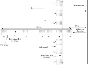
Three directional wave fields were generated. We name the wave fields W1, W2 and W3. Figure 6 shows the locations L1–L12 of the $10\times 10$ array in the basin. The main wave direction was in the $x$ -direction of the basin. The distance from the wave makers to the centre of location L12 was 7.0 m. The length of the synthetic array in the $x$ and $y$ -directions was 25.6 m and 26.8 m, respectively. In the following we consider measurements from two sub-arrays, named sub-array 1 and 2, indicated in figure 6. Sub-array 1 consisted of measurements from locations L1, L2, L3, L4, L8 and L12 along the main wave direction. Sub-array 2 consisted of measurements from locations L5–L11 perpendicular to the main wave direction. For wave fields W1 and W3 only measurements from locations L7–L9 were available perpendicular to the main wave direction.

Figure 6.

Top view of the MARIN basin showing actual ratio between width and length of the synthetic array.

The MARIN wave fields were initialized with a JONSWAP spectrum (2.9)–(2.12) with different directional spreading. Simanesew et al. (Reference Simanesew, Krogstad, Trulsen and Nieto Borge2016) analysed these wave fields with respect to directional spreading and found that even though the waves were generated with frequency-independent directional spreading they naturally evolved into frequency-dependent directional spreading similar to that observed in the ocean.

Table 1 shows initial parameters for W1, W2 and W3 estimated from sub-array 2. The location of sub-array 2 is close to the wave makers and is suitable for obtaining an estimate of initial parameters. From directional data of sub-array 2 we computed $(k_{y},\unicode[STIX]{x1D714})$ -spectra. The $(k_{y},\unicode[STIX]{x1D714})$ -spectra were obtained from uniform discrete Fourier transform of time series and non-uniform discrete Fourier transform (Fessler & Sutton Reference Fessler and Sutton2003) of data along the $y$ -axis. In order to use directional data from all probes in sub-array 2 we computed a collection of $(k_{y},\unicode[STIX]{x1D714};x)$ -spectra from 10 extracts along the $y$ -direction and averaged over $x$ to obtain the $(k_{y},\unicode[STIX]{x1D714})$ -spectrum. Extract number 1 is shown in figure 6 and extracts number 2–10 are those that follow along the $x$ -direction.

The initial peak frequencies $\unicode[STIX]{x1D714}_{p}$ of W1, W2 and W3 were estimated from $\unicode[STIX]{x1D714}$ -spectra obtained from projection of $(k_{y},\unicode[STIX]{x1D714})$ -spectra onto the $\unicode[STIX]{x1D714}$ -axis, and peak wavenumbers $k_{p}=\unicode[STIX]{x1D714}_{p}^{2}/g$ were then obtained from LDR. The peak frequencies $\unicode[STIX]{x1D714}_{p}$ and wavenumbers $k_{p}$ are given in table 1. For W1 the synthetic array covered about $16\unicode[STIX]{x1D706}_{p}$ along the main wave direction and $17\unicode[STIX]{x1D706}_{p}$ perpendicular to the main wave direction. For W2 and W3 the synthetic array covered about $15\unicode[STIX]{x1D706}_{p}$ along the main wave direction and about $16\unicode[STIX]{x1D706}_{p}$ perpendicular to the main wave direction. The non-dimensional water depth $k_{p}h$ was about 20 for W1 and 19 for W2 and W3. The wave fields were generated for $579T_{p}$ . The first $100T_{p}$ and last $429T_{p}$ were removed and the remaining $50T_{p}$ were used for spectral estimates. The spectra were ensemble averaged by 2 non-overlapping intervals of surface elevation of length $25T_{p}$ collected from total time interval of $50T_{p}$ . The time intervals of approximately $25T_{p}$ were smoothed by 10 iterations of a three-point moving average.

Peak frequencies $\unicode[STIX]{x1D714}_{p}$ were also estimated from $\unicode[STIX]{x1D714}$ -spectra obtained from time series at each of the 10 $\times$ 60 probes in sub-array 1. These peak frequencies were similar to those given in table 1 and relatively constant along the basin.

From table 1 we notice that W1, W2 and W3 have identical steepness, practically similar BFI, and noticeably different crest length. The data points of BFI and inverse crest length $L_{c}^{-1}$ from MARIN data are plotted in figure 5 for the simulations with steepness $\unicode[STIX]{x1D716}=0.04$ in § 3. The data points are situated away from highest values of $\unicode[STIX]{x1D6FF}$ , indicating that deviation due to nonlinear evolution should not be observable from the MARIN data. Figure 5 is obtained from simulations of Gaussian spectra while the MARIN data had JONSWAP spectra, nevertheless the comparison should be reasonable for the relatively low BFI and short crests involved.

The steepness was also estimated from time series at each of the $10\times 60$ probes in sub-array 1 and was similar to the steepness estimated from sub-array 2 given in table 1. Thus the wave fields were not attenuated along the main wave direction.

Table 1.

Parameters from the MARIN wave fields estimated from sub-array 2 in the basin: $\unicode[STIX]{x1D714}_{p}$ , peak frequency; $T_{p}$ , peak period; $k_{p}$ , peak wavenumber; $\unicode[STIX]{x1D706}_{p}$ , peak wavelength; $\unicode[STIX]{x1D716}$ , steepness; $\unicode[STIX]{x0394}\unicode[STIX]{x1D714}/\unicode[STIX]{x1D714}_{p}$ , HWHP frequency bandwidth; BFI, Benjamin–Feir index; $L_{c}$ , crest length and $N$ , spreading parameter given for MNLS simulations for initial spectrum (2.9).

Figure 7.

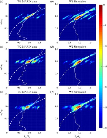
(a,c,e) $(k_{x},\unicode[STIX]{x1D714})$ -spectra obtained from sub-array 1 in the MARIN basin. (b,d,f) $(k_{x},\unicode[STIX]{x1D714})$ -spectra obtained from simulations of the MNLS equation. Colours: spectral energy density in dB. Colour bar in dB. White dashed curve: (4.1). White dotted curves: RMS wavenumber $k_{RMS}$ from (2.14).

Figure 7(a,c,e) shows $(k_{x},\unicode[STIX]{x1D714})$ -spectra of W1, W2 and W3 obtained from sub-array 1. In order to use the directional data from all probes in sub-array 1 we computed a collection of $(k_{x},\unicode[STIX]{x1D714};y)$ -spectra from 10 extracts along the $x$ -direction in the basin and averaged over $y$ to obtain the $(k_{x},\unicode[STIX]{x1D714})$ -spectrum. Extract number 1 is shown in figure 6 and extracts number 2–10 are those that follow along the $y$ -direction. The $(k_{x},\unicode[STIX]{x1D714})$ -spectra were obtained by uniform discrete Fourier transform of the time series and non-uniform discrete Fourier transform (Fessler & Sutton Reference Fessler and Sutton2003) of the data along the $x$ -axis.

The axes of figure 7(a,c,e) are normalized by the peak frequencies $\unicode[STIX]{x1D714}_{p}$ estimated from the $\unicode[STIX]{x1D714}$ -spectra obtained from projection of the $(k_{x},\unicode[STIX]{x1D714})$ -spectra of W1, W2 and W3 onto the $\unicode[STIX]{x1D714}$ -axis, and the peak wavenumbers $k_{p}=\unicode[STIX]{x1D714}_{p}^{2}/g$ from LDR. The peak frequencies $\unicode[STIX]{x1D714}_{p}$ and wavenumbers $k_{p}$ were similar to those given in table 1.

In order to compare distributions of $(k_{x},\unicode[STIX]{x1D714})$ -spectra with linear wave theory we compute

i.e. LDR (1.1) in the limit that $k_{y}=0$ . In figure 7, the white dashed curves show (4.1).

The $(k_{x},\unicode[STIX]{x1D714})$ -spectra from the MARIN data reveal contributions around (4.1) and the peaks of the spectra are in accordance with (4.1). When waves satisfying LDR are projected onto the $(k_{x},\unicode[STIX]{x1D714})$ -plane the curve (4.1) should be a lower bound for contributions in the projected spectral plane. There is no indication of deviation from LDR for the MARIN spectra. Additional distributions are seen away from peak. These are caused by aliasing as a consequence of gaps between the measurement locations in the basin. The white dotted curves show the RMS wavenumber $k_{RMS}$ (2.14). The RMS wavenumber is distributed close to peak but as a consequence of aliasing the estimate of the RMS wavenumber is slightly inaccurate.

Figure 7(b,d,f) shows $(k_{x},\unicode[STIX]{x1D714})$ -spectra obtained from simulations of the MNLS equation. The simulations were initialized with the JONSWAP spectrum (2.9)–(2.12) with $\unicode[STIX]{x1D6FC}$ chosen such that $\unicode[STIX]{x1D716}=0.04$ identical to the steepness of the MARIN wave fields. The directional spreading was determined by the spreading parameter $N$ given for the spreading function $D(\unicode[STIX]{x1D703})$ (2.11). The spreading parameters $N$ that corresponded to $L_{c}$ of the MARIN wave fields were used for simulations and are given in table 1.

The MARIN wave fields were simulated on a computational domain extending over 70 $\unicode[STIX]{x1D706}_{p}$ in both the $x$ and $y$ -directions. A uniform grid of $N_{x}\times N_{y}=512\times 512$ nodes was used. From this domain, sub-domains with spatial coverage identical to that of MARIN sub-array 1 were selected i.e. $16\unicode[STIX]{x1D706}_{p}$ for W1 and 15 $\unicode[STIX]{x1D706}_{p}$ for W2 and W3 along main wave direction. Within the sub-domains the nodes corresponding to gaps between measurement locations in sub-array 1 were removed in order to simulate the non-uniform spatial coverage. The simulated wave fields evolved for 150 $T_{p}$ and as for the MARIN wave fields we removed the first 100 $T_{p}$ and used the next 50 $T_{p}$ for spectral estimates.

Considering the group velocity $\boldsymbol{c}_{g}$ of the peak, the sub-domains were not affected by the periodic boundary conditions of the simulations. Waves leaving the sub-domains would propagate with $\boldsymbol{c}_{g}$ in the full domain without reaching the boundary of the sub-domain during the time of 50 $T_{p}$ used for the spectral estimates.