2. Previous related work

Since the epochal review of Queney (Reference Queney1948) on flow over low and steep hills, the progress of mountain meteorology has been remarkable (Taylor & Teunissen Reference Taylor and Teunissen1987; Blumen Reference Blumen1990; Scorer Reference Scorer1997; Whiteman Reference Whiteman2000). Significant progress has been made on mean flow (synoptic flow driven by large-scale pressure gradients) approaching mountains, especially for neutral (Belcher & Hunt Reference Belcher and Hunt1998) and stably stratified cases (Baines & Manins Reference Baines and Manins1989; Baines Reference Baines1995; Boyer & Davies Reference Boyer and Davies2000). For the neutrally stratified case, the pioneering two-dimensional (2D) linear analysis of Jackson & Hunt (Reference Jackson and Hunt1975) considered low hills with small slopes, say ${<}10^{\circ }$ (Hewer Reference Hewer1998). The analysis has been extended to three-dimensional (3D) cases of practical relevance (Mason & King Reference Mason and King1985; Hunt, Leibovich & Richards Reference Hunt, Leibovich and Richards1988; Carruthers et al. Reference Carruthers, Ellis, Hunt and Chan2012), and the flow features of 2D and 3D cases have been shown to differ substantially (Doyle & Durran Reference Doyle and Durran2007). For steeper slopes without ground heating, the flow separation and a recirculation bubble may appear in the lee of the slope. Weakly (Xu, Ayotte & Taylor Reference Xu, Ayotte and Taylor1994) and full (Apsley & Castro Reference Apsley and Castro1997; Crook & Tucker Reference Crook and Tucker2005) nonlinear models have been developed for flow past idealized topographies, models for flow separation have been developed for non-stratified flows (Lighthill Reference Lighthill and Rosenhead1963), and estimates have been made for the critical slope for flow separation (Wood Reference Wood1995). A number of numerical, field observational and wind tunnel studies on flow separation in neutral flows over topography have been reported (Britter, Hunt & Richards Reference Britter, Hunt and Richards1981; Gong & Ibbetson Reference Gong and Ibbetson1989; also see, Mason & King Reference Mason and King1985; Hunt Reference Hunt1991 and Hewer Reference Hewer1998).

The inclusion of thermal forcing may drastically change the flow character, depending on the competition between ensuing thermal circulation (up/downslope and up/down valley flows) and external flow. A few theoretical studies have been reported in this regard, for both 2D (Raymond Reference Raymond1972; Smith & Lin Reference Smith and Lin1982; Tian & Parker Reference Tian and Parker2003) and 3D (Reisner & Smolarkiewicz Reference Reisner and Smolarkiewicz1994) cases. Using scaling arguments, Mason (Reference Mason1987) derived a form of Froude number that helps delineate convective versus external flow dominated cases, which has broad consistency with that proposed by Lewis et al. (Reference Lewis, Mobbs, Vosper and Brown2008). Numerical studies with periodic 2D hills show that, for low hills, convective flow structures that develop without the external flow are similar to those which appear on flat terrain, but the presence of even a weak mean flow modifies them. When an external mean flow is present, both transverse and longitudinal rolls develop, in contrast to the longitudinal rolls that appear without the mean flow (Dörnbrack & Schumann Reference Dörnbrack and Schumann1993; also see Krettenauer & Schumann Reference Krettenauer and Schumann1989). According to the 2D simulations of Dörnbrack & Schumann (Reference Dörnbrack and Schumann1993), an external flow (with velocity $\overline{U}$ ) may impact on convective structures for $\overline{U}/w_{\ast }>2$ , where $w_{\ast }=(g{\it\alpha}\overline{w^{\prime }T^{\prime }}h)^{1/3}$ is the convective velocity, $g$ gravity, ${\it\alpha}$ the thermal expansion coefficient, $\overline{w^{\prime }T^{\prime }}$ the vertical temperature flux at the surface and $h$ the mean height of the flow, whence the influence of topographic details wanes in determining turbulent statistics of the overlying flow. The cause of the waning is the mean flow which tends to destroy any coherent roll motions induced by the undulating terrain for zero mean flow and therefore reduces the impact of the terrain parameters on the turbulence statistics. They showed that, for low hills of sufficient steepness, heating reduces the likelihood of lee-side flow separation, and the characteristic size and velocity of the separation bubble are reduced when heating is present. This is due to the enhanced vertical momentum diffusion on the windward side of the mountain due to convection, thus reducing the vorticity of the leeward separation bubble (Allen & Brown Reference Allen and Brown2006). On the other hand, for steeper and high topographic features, heating facilitates the lee-side flow separation, and for a given flow velocity and valley width, the separation occurs above a critical heating rate. Lehner & Whiteman (Reference Lehner and Whiteman2012) have studied separation features of idealized basin-shaped topographies using a large-eddy simulation (LES) version the Weather Research and Forecasting (WRF) model. They employed spatial and temporally varying heating, and noted that thermal asymmetry so introduced leads to closed circulations cells that move toward sidewalls of more pronounced heating.

Crook & Tucker (Reference Crook and Tucker2005) demonstrated that flow past a uniformly heated topography, consisting of an obstacle above a flat surface, can be approximated by flow past the topography with heating occurring over the obstacle surface only. They developed linear and nonlinear models and, in the former, flow past a heated low hill could be analysed by superposing the separate responses of thermal and orographic forcing. To our knowledge, no laboratory experiments delving into flow separation in heated mountainous terrain have been reported hitherto, although a number of studies have dealt with flow over a heated uniform slope (Chen et al. Reference Chen, Berman, Boyer and Fernando1996) and complex topography with spatially varying slopes (Berman et al. Reference Berman, Boyer, Brazel, Brazel, Chen, Fernando and Fitch1995; Reuten et al. Reference Reuten, Steyn and Allen2007) in the presence of background stable stratification. The stable stratification appears to have a tendency to suppress flow separation, and this case is relevant to the morning transition in complex terrain during which the nocturnal inversion is destroyed by heating of the ground during sunrise (Lu & Turco Reference Lu and Turco1994; Princevac & Fernando Reference Princevac and Fernando2008). The present paper considers the case without background stratification, which mimics the case of upslope flow after the morning transition.

3. Experiments

The experiments were carried out in a glass tank of rectangular cross-section ( $125~\text{cm}\times 30~\text{cm}$ ) filled with deionized water to a depth of 30 cm. To minimize heat leakage to ambient air, water at the room temperature was used, and 5 cm thick styrofoam thermal insulation encased the tank on all sides. The top insulation isolates the tank from ambient air, thus ensuring two-dimensionality of the flow and absence of secondary circulation. A removable window in the insulation allowed optical access to the flow. A unit serving as a $15.6~\text{cm}\times 30~\text{cm}$ heated slope was custom manufactured, which consisted of an array of densely packed heating wires embedded in silicon rubber. The bottom of the pad was fully insulated. The unit was heated by applying a constant DC current and could attain a maximum possible heat flux of $2.0~\text{kW}~\text{m}^{-2}$ , where the heat flux could be estimated as $Q=IV/A$ , where $I$ is the applied current, $V$ the applied voltage and $A$ the slope area. This estimation was independently verified using the standard calibration techniques described in Hunt, Fernando & Princevac (Reference Hunt, Fernando and Princevac2003).

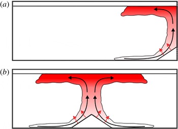
Two experimental configurations were considered, as sketched in figure 1. In the first, the slope was placed abutting the wall (figure 1 a), and by assuming that the no-slip condition plays a lesser role in the overall plume dynamics, the flow was considered similar to the case of a symmetric triangular-shaped mountain (figure 1 b). This assumption is particularly plausible for thicker (vertical) plumes, whence the flow separation is unaffected by the vertical wall. A series of experiments was conducted using both configurations, under otherwise identical conditions, and the separation points observed were within $\pm 5\,\%$ with no particular bias for one case or another. Given that the configuration in figure 1(a) allows longer flow development times before the endwalls become important, the majority of the experiments were conducted using that configuration.

Figure 1.

Schematics of experimental configurations used.

In the experiments, the water tank was allowed to settle for two hours for residual motion to decay, whereupon a prescribed current was applied to the heating elements. Video recordings were made of the initial transients, the quasi-steady current feeding the upslope flow and the flow separation. The experiment was terminated when measurable velocities were detected at the distant endwall. Post-processing of the data allowed identification of a quasi-steady period. The temperature of the sloping surface was obtained using a number of $k$ -type thermocouples. Eleven prescribed slope angles ${\it\beta}=0^{\circ }$ , 5°, 10°, 15°, 18°, 20°, 25°, 30°, 35°, 40° and 45° were used, and the heat flux was varied between $9.4~\text{W}~\text{m}^{-2}$ and $2.0~\text{kW}~\text{m}^{-2}$ .

Flow velocities were measured using particle tracking velocimetry (PTV). The flow was seeded with orange fluorescent polyethylene particles, $90~{\rm\mu}\text{m}$ in diameter and density ${\it\rho}\approx 1~\text{g}~\text{cm}^{-3}$ . A 3 mm thick Ar-ion laser sheet ( $\text{wavelength}\sim 510~\text{nm}$ ), introduced through a vertical slit in the insulation, provided illumination for a vertical cross-section of the flow in the middle of the tank. The spheres are sensitive to a wide range of excitation wavelengths and emit light at ${\sim}600~\text{nm}$ . The particle motions were viewed through an orange filter of cutoff wavelength ${\sim}600~\text{nm}$ to achieve high-contrast images with easy particle detection and processing, while eliminating light from sources other than moving particles. To obtain optimal particle track detection, special attention was paid to ensuring sufficient water clarity and particle seeding density. A $752~\text{pixel}\times 480~\text{pixel}$ CCD camera positioned in front of the observation window was used to record videos of particle motion at 5 f.p.s. The camera was set to capture the flow at the slope and its immediate vicinity at $35{-}54~\text{pixel}~\text{cm}^{-1}$ spatial resolution. Recorded videos were split into individual frames and processed by in-house-developed PTV software. Image enhancement was first applied to improve the contrast as well as for spatial filtering. Individual particles were then detected in each frame, allowing reconstruction of 2D particle motions. In later stages of data processing, the velocity components were calculated using track information.

To confirm that the insulation was sufficient, numerous vertical and horizontal cross-sections of the flow were imaged and analysed using PTV for experiments with different slope angles. The horizontal flow in the far field, especially in the central region of the tank, and its modification when approaching the near field of the slope were interrogated. Particle tracks and velocity components allowed detection of the distance $L_{s}$ along the slope at which the flow separates as well as calculation of the mean local velocity $U_{s}$ at the separation point.

The distance $L_{s}$ was detected by examining a map of particle tracks and with the help of feature tracking visualizations (FTV). The latter reconstructed particle paths by colour mapping them according to the track length and/or velocity, thus providing a good representation of the time history of the flow. A combination of static paths maps and FTV animations allowed confident detection of $L_{s}$ with acceptable accuracy, which is discussed further in § 6.1. The values of $U_{s}$ were then obtained by ensemble-averaging velocities in the vicinity of the separation point. Wherever possible, the uncertainties were estimated using the technique of Kline & McClintock (Reference Kline and McClintock1953).

4. Experimental observations

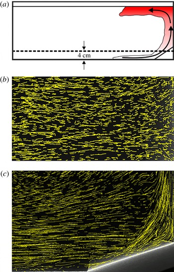
Observations were made from the initiation of heating until the plume recirculation flow reached the opposite tank wall. At first, small-scale roll structures appeared on the slope that broke down to form an upslope flow that separated, rose vertically, deflected from the top surface and flowed horizontally as an intrusion (figure 1). This transition period lasted for up to 200 s, but it varied with the experimental parameters, i.e. the higher the buoyancy flux, the shorter the transient period. As the plume intrusion gradually propagated into the tank interior, the upslope flow and the plume generated by its separation underwent a quasi-steady period. During this period, the upslope flow, rising plume and the resulting intrusion developed without any apparent influence of the endwalls. When the endwall influence sets in, a large quasi-stationary cell developed in the tank that clearly affected flow in the tank, including the upslope flow. All phases of flow evolution were observed by PTV-track maps constructed from intervals of 250 images (50 s based on 5 f.p.s.); see figure 2. Reuten et al. (Reference Reuten, Steyn, Strawbridge and Bovis2005) hypothesized that a recirculating flow may develop surrounding the upslope flow, thus trapping fluid parcels in a cell above the slope. Such closed-loop circulation was not observed in the present case; instead the upslope flow was fed by the lateral entrainment. The slope flow separated at a distance $L_{s}$ from the mountain foot, and lofted the buoyant fluid.

Figure 2.

Particle tracks at an illuminated cross-section, which shows an approach flow, parallel to the walls ( ${\it\beta}=20^{\circ }$ ). The dashed line in (a) is the location of (b), the horizontal cross-section 4 cm above the bottom. (c) The vertical cross-section passing through the tank centre in its long direction.

Figure 2(b) shows PTV pathlines obtained in the plan view by illuminating a horizontal cross-section at a representative height of 4 cm above the bottom (figure 2 a). The corresponding vertical cross-section through the centre of the tank is given in figure 2(c). Observations at several other horizontal planes also exhibited similar characteristics (not shown). Note the 2D nature of the flow, except near the tank walls where some deviations could be seen (figure 2 b). Given the 2D nature, particles could be tracked throughout the field of view, providing long pathlines. Of course, two-dimensionality is less evident near the slope, where the flow is complicated by turbulent upslope flow, separation and plume formation.

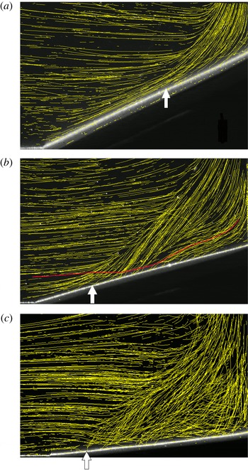
An interesting observation was the response of slope flow to varying slope angle ${\it\beta}$ . When ${\it\beta}>{\it\beta}_{c}~({\approx}20^{\circ })$ , the flow consisted of upslope flow at low elevations, flow separation at $L_{s}$ , and a rising plume fed by the separated upslope flow (figure 3 a). Up to some vertical distance from the location of formation (i.e. region of flow separation), the plume is mainly driven by the buoyancy of fluid parcels, aided by the initial vertical momentum of fluid parcels that arise from the antecedent upslope flow. The rising plume away from the source region is fed by fluid entraining from the surroundings, which approaches the rising plume almost horizontally.

Figure 3.

A track map extracted from an FTV animation. It illustrates the long-exposure pathlines of fluid parcels: (a)  ${\it\beta}=25^{\circ }$ , (b)  ${\it\beta}=15^{\circ }$ , (c)  ${\it\beta}=5^{\circ }$ . The white arrow represents the estimated separation point. Note that in (a) very few outside parcels penetrate the plume core, causing upslope flow to feed the plume entirely, whereas in (b,c) there is substantial penetration as illustrated by the red particle track in (b).

It is well known that when a buoyant fluid with some initial vertical momentum is released, the incipient motion is momentum dominated (as in the case of a jet), and after rising to the momentum length $L_{M}$ the motion becomes buoyancy dominated (behaves as a plume); see List (Reference List1982) and Papanicolaou & List (Reference Papanicolaou and List1988). For the present 2D case, the momentum length scale becomes $L_{M}=M_{0}/B_{0}^{2/3}$ , where the plume source following flow separation has a total vertical kinematic momentum flux per unit width $M_{0}$ and a buoyancy flux $B_{0}$ (also see § 5). Typical values of $L_{M}$ for the present experiments are on the order of 4 cm.

As ${\it\beta}$ decreases, the separation point recedes, arriving at a scenario where the upslope flow is not sufficiently developed to supply fluid to the separated plume, as shown in figure 3(b). This appears at ${\it\beta}\leqslant {\it\beta}_{c}$ (figure 3 b), and appreciable entrainment of outside flow into the core of the plume could be observed at the level of plume formation, together with the increasing 3D nature of the flow. Further reduction of ${\it\beta}$ completely eliminated the upslope flow, which was observed when ${\it\beta}\leqslant 10^{\circ }$ , whereupon the flow is much like a plume from a horizontal source of finite dimensions; see figure 3(c). Note that, in the near field, 2D plumes of finite width are different from those of zero width (line plumes). Colomer, Boubnov & Fernando (Reference Colomer, Boubnov and Fernando1999) have studied the former for the axisymmetric case and Rouse, Yih & Humphreys (Reference Rouse, Yih and Humphreys1952) reported a comprehensive study on the latter. The development of a simple theoretical model followed the experimental observations and is described next.

5. Model

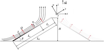
Consider a 2D upslope flow that develops on a uniformly heated incline of length $L_{0}$ and of slope angle ${\it\beta}$ described by along-slope ( $s$ ), slope-normal ( $n$ ) and $y$ coordinates as shown in figure 4. The ambient fluid is neutrally stratified, approximately mimicking quiescent atmospheric cases after the breakup of inversions (Pardyjak et al. Reference Pardyjak, Fernando, Hunt, Grachev and Anderson2009). The flow starts developing at the base of the incline as an upslope flow, entraining fluid from the surroundings. As the flow develops along the slope with upslope velocity $u$ in the $s$ direction, the heating of the incline amplifies the baroclinic torque ( $\boldsymbol{{\rm\nabla}}\times b\hat{\boldsymbol{k}}$ ) that counters the vorticity advection by the shear flow ( $\boldsymbol{u}\boldsymbol{\cdot }\boldsymbol{{\rm\nabla}}{\bf\omega}$ ), thus facilitating the flow separation. These competing terms appear in the vorticity ( ${\bf\omega}$ ) equation (to the Boussinesq approximation) as

(5.1) $$\begin{eqnarray}\frac{\partial {\bf\omega}}{\partial t}+\boldsymbol{u}\boldsymbol{\cdot }\boldsymbol{{\rm\nabla}}{\bf\omega}={\bf\omega}\boldsymbol{\cdot }\boldsymbol{{\rm\nabla}}\boldsymbol{u}+\boldsymbol{{\rm\nabla}}\times (b\hat{\boldsymbol{k}})+{\it\nu}{\rm\nabla}^{2}{\bf\omega},\end{eqnarray}$$

where ${\it\nu}$ is the viscosity, $\boldsymbol{u}$ the velocity, $b$ the buoyancy $b=g({\it\rho}_{0}-{\it\rho})/{\it\rho}_{0}$ , ${\it\rho}$ the density, ${\it\rho}_{0}$ a reference density, $g$ gravity and $t$ the time. The $y$ component of vorticity ${\it\omega}_{y}$ becomes

(5.2) $$\begin{eqnarray}\frac{\partial {\it\omega}_{y}}{\partial t}=(\boldsymbol{{\rm\nabla}}\times b\hat{\boldsymbol{k}})_{y}-u\frac{\partial {\it\omega}_{y}}{\partial s}.\end{eqnarray}$$

Assuming Reynolds number similarity, the viscous influence can be neglected. At the separation point the opposing vorticities balance, and $u\partial {\it\omega}_{y}/\partial s\sim (\boldsymbol{{\rm\nabla}}\times b\hat{\boldsymbol{k}})_{y}$ , with $(\boldsymbol{{\rm\nabla}}\times b\hat{\boldsymbol{k}})_{y}=-\partial (b\cos {\it\beta})/\partial s$ . Using the scaling $u\sim U$ , $b\sim {\rm\Delta}b$ , ${\it\omega}_{y}\sim {\it\omega},\partial /\partial n\sim 1/{\it\delta}$ and $\partial /\partial s\sim 1/s$ , where ${\it\delta}$ is the upslope-layer thickness (that grows along the slope), the vorticity scaling at separation becomes ${\it\omega}_{y}\sim {\rm\Delta}b\cos {\it\beta}/U$ . At the separation point, ${\it\omega}_{y}$ generated by buoyancy is balanced by that due to boundary-layer shear, ${\it\omega}_{y}=\partial u/\partial n\sim U/{\it\delta}$ . Using subscript $s$ to denote the separation point, the condition for the upslope flow separation can be written as ${\it\omega}_{s}\sim {\rm\Delta}b_{s}\cos {\it\beta}/U_{s}\sim U_{s}/{\it\delta}_{s}$ or

(5.3) $$\begin{eqnarray}U_{s}^{2}\sim {\rm\Delta}b_{s}\cos {\it\beta}{\it\delta}_{s}.\end{eqnarray}$$

Using the approximate buoyancy conservation equation, $\partial (bu{\it\delta})/\partial s\approx q_{0}$ , where $q_{0}=g{\it\alpha}Q/{\it\rho}_{0}C_{p},~Q$ the heat flux per unit area and $C_{p}$ the specific heat (Schumann Reference Schumann1989), an additional scaling equation is possible,

(5.4) $$\begin{eqnarray}{\rm\Delta}b_{s}U_{s}{\it\delta}_{s}\sim q_{0}L_{s},\end{eqnarray}$$

where $L_{s}$ is the separation length. From (5.3) and (5.4), the upslope velocity at the flow separation becomes

(5.5) $$\begin{eqnarray}U_{s}\sim (q_{0}L_{s}\cos {\it\beta})^{1/3}.\end{eqnarray}$$

Figure 4.

A schematic of the upslope flow. At the flow separation, the flow rises as a plume that is fed by the anabatic flow.

A velocity scale for upslope flows has been derived by Hunt et al. (Reference Hunt, Fernando and Princevac2003), by considering a steady turbulent shear flow generated by heating an incline. Their model consisted of several layers with disparate dynamics, each having an intrinsic transport mechanism. The velocity scale so derived, $U\sim (q_{0}{\it\delta}\sin {\it\beta})^{1/3}$ , is expected to be valid up to flow separation. Equating the two estimates at the separation point, we get $L_{s}/{\it\delta}_{s}\sim \tan {\it\beta}$ . Field and laboratory observations show that the separated flow rises as a plume formed in the region between the separation point and the apex of the slope (see § 6.3), for example, as shown in figures 2–4. The volume flux of the plume is mainly fed by the anterior anabatic flow (e.g. Geerts, Miao & Demko Reference Geerts, Miao and Demko2008), as was evident from the present experiments at higher slopes ${\it\beta}>{\it\beta}_{c}$ . The total buoyancy flux fed into the plume is $B_{0}=q_{0}L_{t}$ , where $L_{t}=L_{0}-L_{s}$ , and the buoyancy flux over an equivalent horizontal plane is

(5.6) $$\begin{eqnarray}q_{0}^{\ast }=\left(\frac{q_{0}L_{t}}{L_{t}\cos {\it\beta}}\right),\end{eqnarray}$$

where we have assumed that the effect of the total buoyancy flux emanating from the slope is equivalent to that of a horizontal source with the same total buoyancy flux distributed uniformly. The buoyancy $(b)$ , vertical velocity $(w)$ , and near-field entrainment velocity $(u_{e})$ scaling for horizontal plume sources of finite dimensions $(L_{w})$ driven by a buoyancy flux ( $q_{0}^{\ast }$ ) has been proposed by Colomer et al. (Reference Colomer, Boubnov and Fernando1999), which is a variant of the well-known scaling for point and line plumes (List Reference List1982). For 2D horizontal sources of finite source dimensions, the analogous 2D near-field scaling can be readily written as

(5.7a−c ) $$\begin{eqnarray}b\sim \frac{(q_{_{0}}^{\ast }L_{w})^{2/3}}{L_{w}},\quad w\sim (q_{_{0}}^{\ast }L_{w})^{1/3}\quad \text{and}\quad u_{e}\sim (q_{_{0}}^{\ast }L_{w})^{1/3}.\end{eqnarray}$$

The vertical plume velocity in the proximity of the finite-width source generated by flow separation now becomes $w_{s}\sim (q_{0}^{\ast }L_{t}\cos {\it\beta})^{1/3}$ , where the source half-width of the 2D plume is $L_{w}=L_{t}\cos {\it\beta}$ . Using (5.6) and (5.7), the vertical plume velocity scale can be written as $w_{s}\sim (q_{0}L_{t})^{1/3}$ .

As discussed in § 4, when there is initial momentum to the buoyant fluid, the rising flow is transformed into a true buoyant plume after a vertical distance of $L_{M}=M_{0}/B_{0}^{2/3}$ , and for the present case $M_{0}\approx U_{s}^{2}{\it\delta}_{s}\sin {\it\beta},~B_{0}\approx q_{0}L_{t}$ and thus $L_{M}\sim L_{s}(L_{s}/L_{t})^{2/3}\cos ^{4/3}{\it\beta}$ . Note that (5.7) is strictly valid beyond $L_{M}$ (which is suitably small in our cases), and hence in comparing with (5.7), the velocity measurements need to be taken at an appropriate distance from the flow separation location.

It is assumed that for ${\it\beta}>{\it\beta}_{c}$ the total vertical volume flux of the plume at the separation location ${\sim}(q_{0}L_{t})^{1/3}L_{t}\cos {\it\beta}$ is balanced by the along-slope volume flux of the anabatic flow ${\sim}U_{s}{\it\delta}_{s}$ that feeds the plume. Equating the two fluxes at the point of separation, $U_{s}{\it\delta}_{s}\sim (q_{0}L_{t})^{1/3}L_{t}\cos {\it\beta}$ and using (5.5) and $L_{s}+L_{t}=L_{0}$ , an expression for $L_{s}/L_{0}$ is obtained,

(5.8) $$\begin{eqnarray}\frac{L_{s}}{L_{0}}=\left[1+{\it\Pi}\frac{\sin ^{1/4}2{\it\beta}}{\sin {\it\beta}}\right]^{-1},\end{eqnarray}$$

where ${\it\Pi}$ is a proportionality constant arising from the scaling. From (5.8), it is evident that $L_{s}/L_{0}$ has a weaker dependence on ${\it\beta}$ at large ${\it\beta}$ . Also note that (5.8) is a definitive form of the functional relationship obtained from straightforward dimensional analysis, $L_{s}=f(q_{0},L_{0},{\it\beta},{\it\nu})$ . With ${\it\beta}={\it\beta}(L_{0},H)$ , where $H$ is the summit height,

(5.9) $$\begin{eqnarray}\frac{L_{s}}{L_{0}}=f_{1}\left(\frac{H}{L_{0}},\mathit{Re}_{H}\right)\rightarrow f_{2}\left(\frac{H}{L_{0}}\right)=f_{2}({\it\beta}),\end{eqnarray}$$

for large $\mathit{Re}_{H}=(q_{0}H)^{1/3}H/{\it\nu}$ , where $f_{1}$ and $f_{2}$ are functions. Note that $\mathit{Re}_{H}$ is an implicit form of the Reynolds number. At large $\mathit{Re}_{H}$ the Reynolds number similarity follows, hence causing $f_{1}$ to be independent of $\mathit{Re}_{H}$ . Since $\mathit{Re}_{H}$ is defined in terms of bulk parameters, it does not explicitly represent the velocity and length scales or slope angle dependence. Alternatively, a Reynolds number $\mathit{Re}_{U}$ can be defined in terms of the scales at flow separation, i.e.  $\mathit{Re}_{U}=U_{s}{\it\delta}_{s}/{\it\nu}$ , which is related to $\mathit{Re}_{H}$ .

Recall that the above formulation is valid for ${\it\beta}>{\it\beta}_{c}$ , and in § 4 it was pointed out that in the limit ${\it\beta}\rightarrow 0$ the flow approaches that of a uniformly heated horizontal plume source of finite width ( $L_{w}\approx L_{0}$ ), where scaling (5.7) is applicable. In this regime the slope is sufficiently small (or below a critical slope ${\it\beta}_{u}$ ) to suppress the upslope flow. According to the measurements and theoretical arguments of Princevac & Fernando (Reference Princevac and Fernando2007), for a given fluid, ${\it\beta}_{u}(\mathit{Pr})$ is fixed, being dependent only on the Prandtl number $\mathit{Pr}$ for the case of upslope flows starting from rest.

As discussed by Colomer et al. (Reference Colomer, Boubnov and Fernando1999), a plume of finite width recedes toward its centre from the edge of the source. This is nominally a flow separation region occurring due to horizontal entrainment flow into the plume that overshadows rising thermals at its edge (figure 3 c). The characteristic lateral penetration (or separation) distance $L_{s}$ of the entrainment flow before the liftoff can be estimated using the vertical momentum equation, by considering a balance of buoyancy forces due to heating of the entrainment flow and the vertical inertia forces, viz.

(5.10) $$\begin{eqnarray}b\sim \frac{\text{D}w}{\text{D}t}\sim u\frac{\partial w}{\partial x}\sim \frac{u_{e}w}{L_{s}}\sim \frac{{\it\alpha}_{1}w^{2}}{L_{s}},\end{eqnarray}$$

where $L_{s}$ is the separation distance from the edge, $w$ the vertical velocity outside the thermal boundary layer, $u_{e}={\it\alpha}_{1}w$ the entrainment velocity, and ${\it\alpha}_{1}$ the entrainment coefficient for 2D plumes (according to Rouse et al. Reference Rouse, Yih and Humphreys1952, for 2D line-source plumes, ${\it\alpha}_{1}\approx 0.25$ ). Note that this estimation is valid above the boundary-layer region of entrainment flow arriving at the heated surface. Together, (5.10) and (5.7) give

(5.11) $$\begin{eqnarray}L_{s}\sim {\it\alpha}_{1}L_{0}.\end{eqnarray}$$

The detailed predictions made in this section are evaluated against experimental data in § 6.

6. Experimental measurements

6.1. Separation length

To obtain a quasi-steady flow with minimum endwall influence for a reasonable period, a particular range of buoyancy fluxes $q_{0}$ was necessary, and our study focused only on such cases. For $q_{0}$ below this range, the flow either developed eddies that rolled up the slope (similar to laminar convection on slopes; Chen et al. Reference Chen, Labhabi, Chang and Kelly1991) or circulated in a counterclockwise direction as a single stationary eddy of size approximately equal to the depth of the tank. When conditions for quasi-steady upslope flow prevailed, the mean flow was slope-parallel, with entrainment at its edges, and flow separation occurred at a distance $L_{s}$ from the bottom (figure 3 a). Small fluctuations in the separating flow paths were detected, confirmed by releasing small amounts of fluorescent dye on the slope and by FTV animations.

The distance to the separation point $L_{s}$ was detected for each of the examined cases, and was determined by manually examining particle tracks obtained from PTV and selecting the point of the first visible track separation from the slope. The detected separation point location was then verified, and corrected if necessary, by examination of FTV animations. A combination of both the static map of particle tracks and FTV animations provided an accurate detection of $L_{s}$ . The position error was estimated to be less than the distance travelled by a particle during three consecutive frames, ${\rm\Delta}L_{s}=\pm 3{\rm\Delta}tU_{s}$ , where ${\rm\Delta}t$ is the time delay between the frames, based on the image acquisition frame rate of 5 f.p.s.

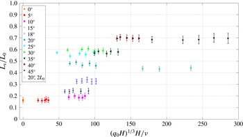
Figure 5 shows the dimensionless separation distance $L_{s}/L_{0}$ as a function of $\mathit{Re}_{H}=(q_{0}H)^{1/3}H/{\it\nu}$ for all of the examined slope angles ${\it\beta}$ . A reasonable parameter range could be obtained by varying the buoyancy flux $q_{0}$ . The estimated errors of $L_{s}/L_{0}$ were ${\sim}10\,\%$ for lower $\mathit{Re}_{H}$ and less than 3 % for higher $\mathit{Re}_{H}$ , and are presented as error bars. The separation distance increased with the slope angle, from $0.16L_{0}$ for 5° and up to $0.7L_{0}$ for the largest examined angle of 45°. With the decrease of ${\it\beta}$ , a higher $q_{0}$ was required to initiate the upslope flow. The results show that, at each angle, the separation distance is virtually a constant and therefore is $\mathit{Re}_{H}$ independent at all ranges of $\mathit{Re}_{H}$ . This confirms the Reynolds number similarity assumption made in (5.2).

Figure 5.

Dimensionless flow separation distance $L_{s}/L_{0}$ as a function of $\mathit{Re}_{H}$ . The calculation of error bars is given in § 6.1. The ♢ symbols show the double slope configuration data (figure 1 b).

Next, a double slope configuration was used, as in figure 1(b), with each slope having a length of 15.6 cm. The measurements were performed at slope angles of 20° and 30°, resulting in similar $L_{s}/L_{0}$ values (within $\pm 5\,\%$ ) to those presented in figure 5; the corresponding data points for ${\it\beta}=20^{\circ }$ are included in figure 5. The double slope, however, increased the rising flux of buoyant fluid above the slope, causing the rapid formation of a thick, warm layer at the top, which violated the assumption of constant background density. Therefore, results from the double slope were limited to a few cases.

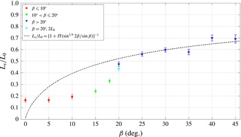
The measured normalized separation lengths are shown in figure 6 as a function of ${\it\beta}$ , together with the prediction (5.8). The model and the data agreed well for ${\it\beta}>20^{\circ }$ , with ${\it\Pi}=0.35$ but below the critical inclination ${\it\beta}_{c}\approx 20^{\circ }$ , the model overpredicted the separation length. The data show a sharp drop of $L_{s}/L_{0}$ for $20^{\circ }\geqslant {\it\beta}>10^{\circ }$ and an approximately constant $L_{s}/L_{0}\approx 0.2$ for ${\it\beta}\leqslant 10^{\circ }$ . Based on the observations discussed in § 4, this can be attributed to the transition from a flow where the upslope flow supplies the entire volume flow of the separated plume ( ${\it\beta}>{\it\beta}_{c}$ ) to one where the source region of the separated plume draws volume flux from both the upslope flow and background ( ${\it\beta}\leqslant {\it\beta}_{c}$ ). The weak variation of $L_{s}/L_{0}$ with ${\it\beta}$ for ${\it\beta}\leqslant 10^{\circ }$ can be construed as due to the approach of the horizontal-plume regime, as discussed in § 4. In this case, the contribution of the upslope flow is unimportant and the plume rises from almost the entire slope length. The estimation (5.11) for this case, $L_{s}\sim {\it\alpha}_{1}L_{0}$ , is in good agreement with the observations of figure 6 that show $L_{s}/L_{0}\approx 0.16$ for ${\it\beta}\leqslant 10^{\circ }$ . This is consistent with entrainment coefficients ${\it\alpha}_{1}$ for horizontal line plumes ( ${\it\alpha}_{1}\approx 0.25$ ), yielding an $O(1)$ proportionality constant of 0.65 for (5.11).

Figure 6.

Ensemble-averaged dimensionless separation length $L_{s}/L_{0}$ as a function of the slope angle ${\it\beta}$ . The dashed line represents the separation length prediction (5.8) with ${\it\Pi}=0.35$ .

As stated in § 5, the formation of upslope flow on an inclined heated slope is possible when ${\it\beta}>{\it\beta}_{u}(\mathit{Pr})$ , and for the present work, based on the model of Princevac & Fernando (Reference Princevac and Fernando2007), ${\it\beta}_{u}\approx 5^{\circ }$ . This is broadly consistent with the observation that the pure plume regime is originated for ${\it\beta}\leqslant 10^{\circ }$ , taking into account that Princevac & Fernando (Reference Princevac and Fernando2007) considered the (transient) case of initial upslope flow formation from rest and the present work deals with plumes at the steady state. Also note the narrow regions of figure 6 where constant $L_{s}/L_{0}$ can be identified even for ${\it\beta}>{\it\beta}_{c}$ . In such regions, we have not been able to observe any mechanistic changes to the flow or systematic departure of data from the model. Therefore, we have not placed an emphasis on such observations.

6.2. Velocity magnitude

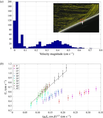
A small rectangular region of interrogation ( $\pm 0.4~\text{cm}$ ) around the detected point of separation was chosen to obtain the local mean velocity magnitude at the point of separation $U_{s}$ . To ensure the full inclusion of the near-slope boundary layer, the rectangle included a portion of the slope itself, resulting in a partial combination of raw velocity data with some falsely detected values. Particle velocities were calculated in this region by dividing digitized track lengths between two consecutive frames by the frame rate value (5 f.p.s.). A representative histogram of calculated velocity magnitudes is shown in figure 7(a).

Figure 7.

(a) Velocity magnitude distribution histogram at the point of separation. Inset figure shows an example of the small region of interest that was chosen in the vicinity of the point of separation ( ${\it\beta}=20^{\circ }$ ). (b) Local mean upslope velocity, $U_{s}$ , at the point of flow separation. Dashed line is a linear fit (5.5) with the proportionality constant ${\it\gamma}=U_{s}/(q_{0}L_{s}\cos {\it\beta})^{1/3}=4.9$ . The calculation of error bars is given in § 6.2.

The main ensemble of velocity magnitudes was distributed in an approximate bell shape, close to a normal distribution, as seen in the histogram. The velocity values on either extreme of the distribution were filtered out from the ensemble; they were attributed to false particle detection at the slope surface caused by the laser sheet reflection and particles outside the separation region. This filtering method allowed an accurate measurement of the velocity; based on the particle position detection accuracy of $\pm 0.5~\text{pixels}$ , spatial resolution $35{-}54~\text{pixel}~\text{cm}^{-1}$ and a frame rate of 5 f.p.s., errors are estimated to be from 6.8 % to 10 %.

In the analysis, interestingly, the along-slope velocities at the separation point $U_{s}$ were found to fall into three distinct regimes, consistent with those identified in § 4. All data for ${\it\beta}>{\it\beta}_{c}~({\approx}20^{\circ })$ followed (5.5), with a proportionality constant of 4.9, as shown in figure 7(b) as a plot of $U_{s}$ versus $(q_{0}L_{s}\cos {\it\beta})^{1/3}$ . The data at ${\it\beta}=25^{\circ }$ show some deviation from the data cluster of ${\it\beta}>20^{\circ }$ , perhaps indicating a gradual move toward a different dynamical regime that onsets between ${\it\beta}=20^{\circ }$ and 25°. The deviation, however, remains within the error bars and hence definite conclusions could not be made on the departure. Also evident is the clustering of data for $15^{\circ }\leqslant {\it\beta}\leqslant 20^{\circ }$ , which is the transition regime wherein the separated plume could not be supplied only via the upslope flow. Results for ${\it\beta}\leqslant 10^{\circ }$ also showed a distinct cluster, arguably approaching the case of plumes from horizontal sources of finite size (figure 3 c). The data therein follow (5.7), with $U_{s}$ being the lateral entrainment flow, $U_{s}\sim (q_{0}L_{s}\cos {\it\beta})^{1/3}\approx (q_{0}L_{0})^{1/3}$ for small ${\it\beta}$ . This is also equivalent to $U_{s}\sim (q_{0}L_{s}\cos {\it\beta})^{1/3}$ , which is supported by figure 7(b), given that $L_{s}\sim L_{0}$ .

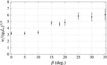
To further corroborate the velocity scaling for plumes after flow separation, the ensemble-averaged dimensionless vertical velocity (following from figure 7), $w/(q_{0}L_{t})^{1/3}$ , of the plume versus ${\it\beta}$ is shown in figure 8. These measurements were taken at a distance $z=z_{m}=0.3L_{t}\cos {\it\beta}$ above the slope apex, where $L_{t}\cos {\it\beta}$ is the plume half-width. The selection of $z_{m}$ followed the inferences of Colomer et al. (Reference Colomer, Boubnov and Fernando1999) that it is within the near field of the plume source where (5.7) holds and that it approximately satisfies the momentum length scale $L_{M}$ criterion of § 5 ( $L_{M}\sim 4~\text{cm}$ ). For ${\it\beta}\leqslant 10^{\circ }$ , $L_{t}\approx 0.8L_{0}$ , the flow behaves as a plume of finite diameter and $w$ scales as (5.7). In $10^{\circ }<{\it\beta}\leqslant 20^{\circ }$ , the flow is in a transition regime and with increasing ${\it\beta}$ the flow approaches another regime with $w/(q_{0}L_{t})^{1/3}\approx 6$ , supporting the underlying arguments of the model developed in § 5.

Figure 8.

Ensemble-averaged dimensionless vertical velocity, $w/(q_{0}L_{t})^{1/3}$ , of the plume at $z=0.3L_{t}\cos {\it\beta}$ above the slope apex as a function of ${\it\beta}$ . Here $w$ is the plume velocity outside the thermal boundary layer and $L_{t}\cos {\it\beta}$ is the plume half-width. Data beyond the 35° angle were unusable, because the field of PTV visualization did not capture a reasonable area near the plume source.

6.3. Field measurements

The field experiments were conducted at the GMAST of the US Army Dugway Proving Ground, Utah, as a component of the MATERHORN Program (for details see Fernando & Pardyjak Reference Fernando and Pardyjak2013). GMAST is centred around a single isolated (Granite) mountain, which is on average 11.8 km long, 6.1 km wide and 0.6 km high. The area surrounding the mountain was densely instrumented with a suite of point and remote sensors (Fernando et al. Reference Fernando, Pardyjak, Di Sabatino, Chow, Fernando, Pardyjak, Di Sabatino, Chow, De Wekker, Hoch, Hacker, Pace, Pratt, Pu, Steenburgh, Whiteman, Wang, Zajic, Balsley, Dimitrova, Emmitt, Higgins, Hunt, Knievel, Lawrence, Liu, Nadeau, Kit, Blomquist, Conry, Coppersmith, Creegan, Felton, Grachev, Gunawardena, Hang, Hocut, Huynh, Jeglum, Jensen, Kulandaivelu, Lehner, Leo, Liberzon, Massey, McEnerney, Pal, Price, Sghiatti, Silver, Thompson, Zhang and Zsedrovits2015). Observations were made during two major field experiments conducted during October 2012 and May 2013. Climatologically, the autumn experiment was intended to study quiescent days characterized by high pressure (low synoptic) conditions and the spring campaign was focused on synoptic days characterized by significant background winds.

Figure 9.

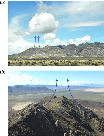
Granite Mountain, Utah with (a) frequently occurring solitary cumulus cloud formation directly over the peak (Courtesy: L. S. Leo) and (b) the LiDAR scan location revealing the quasi-symmetry.

During quiescent days with moderate to high sunshine and sufficient moisture, a solitary cumulus cloud was almost always observed directly above a peak of the Granite Mountain (figure 9 a), indicating the possibility of a separated flow from below. Upon further investigation it was found that the peak is quasi-symmetric (figure 9 b), the slope was nominally 2D over horizontal distances of ${\sim}1.5~\text{km}$ , and the north to south peak orientation provided equivalent early afternoon eastern and western slope sun exposure, thus satisfying the model assumptions of § 5 to a reasonable degree. Although the site was not in the experimental plan for siting instrumentation, special arrangements were made during the spring campaign to relocate a Doppler LiDAR (laser-Radar) to this site for a limited time for observations outside (synoptic-wind focused) the intense observational periods. The number of low-synoptic days with useful data, however, was limited during the spring experiments. Anticipating stronger winds, the tethered balloon flights were not included as part of the spring instrumentation. As such, the background stratification could not be measured directly, but a microwave radiometer located 15 km away in the valley indicated that the boundary layer was well mixed up to about 2 km on the days of measurements. Data on a suite of meteorological towers and remote sensors are available from all of the MATERHORN experiments, and are presented elsewhere (Fernando et al. Reference Fernando, Pardyjak, Di Sabatino, Chow, Fernando, Pardyjak, Di Sabatino, Chow, De Wekker, Hoch, Hacker, Pace, Pratt, Pu, Steenburgh, Whiteman, Wang, Zajic, Balsley, Dimitrova, Emmitt, Higgins, Hunt, Knievel, Lawrence, Liu, Nadeau, Kit, Blomquist, Conry, Coppersmith, Creegan, Felton, Grachev, Gunawardena, Hang, Hocut, Huynh, Jeglum, Jensen, Kulandaivelu, Lehner, Leo, Liberzon, Massey, McEnerney, Pal, Price, Sghiatti, Silver, Thompson, Zhang and Zsedrovits2015).

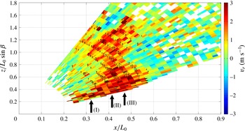
The LiDAR was positioned at the base of the slope, and was aligned to continuously scan parallel to the mean upslope flow direction, sweeping from the base of the incline towards the peak and beyond, with each scan taking 17 s to complete. There were only three days of low-synoptic conditions during the deployment period. Since the LiDAR beam scan is parallel to the mean flow direction, the ( $x,z$ ) flow components ( $u,w$ ) can be projected onto the measured radial Doppler velocity, $u_{r}=u\cos {\it\theta}+w\sin {\it\theta}$ , where ${\it\theta}$ is the scanner elevation angle from the horizontal. Within the upslope flow boundary layer, $w$ can be assumed small such that the upslope velocity $U\sim u_{r}/\cos ({\it\theta}-{\it\beta})$ , while outside the upslope flow boundary layer, the upslope velocity goes to zero and $w\sim u_{r}/\sin \,{\it\theta}$ . A LiDAR scan of the separating upslope flow is shown in figure 10, in which the radial velocity is coloured while the vectors are overlaid to show the approximate direction of the flow. The determination of the separation point is somewhat subjective as evident from figure 10, due to the limitations of measurement resolution near the surface; we therefore opted to estimate the separation point as the location where the maximum vertical velocity is first found.

Figure 10.

Doppler wind LiDAR scan of separating upslope flow, where the radial velocity is coloured with vectors overlaid. No vectors are presented where neither $u$ nor $w$ can be neglected. The flow can be decomposed into three zones, (I) the upslope flow, (II) approximate separation point and (III) plume region. The data were taken on 30 May 2013.

The estimated dimensionless separation distance is $L_{s}/L_{0}=0.45\pm 0.025$ ( $\pm 1$ LiDAR range gate), where the slope length is $L_{0}=712~\text{m}$ . Observations over three days of cumulus formation confirmed the separation distance result within 10 %. Comparison with the model, however, is somewhat problematic, given the change of slope angle in the field from ${\it\beta}=16.5^{\circ }$ at the base to ${\it\beta}=23^{\circ }$ at the peak, a complication that is absent in the model. A possibility is to use a mean slope, ${\it\beta}=19.8^{\circ }$ , and evaluate the separation distance using (5.8) as $L_{s}/L_{0}=0.52$ with an uncertainty of $\pm 0.02$ . Nonetheless, as kindly pointed out by a referee, the model is invalid for ${\it\beta}\leqslant 20^{\circ }$ , and hence it more appropriate to use the empirically determined separation distance for ${\it\beta}\approx 20^{\circ }$ based on figure 6, which is $L_{s}/L_{0}\approx 0.47\pm 0.02$ . Although the agreement is excellent, it should be viewed with circumspection because of the complicating factors present, such as variable slope, possible influence of atmospheric stability particularly at greater elevations and the slope roughness in nature that might increase the boundary-layer thickness (Britter et al. Reference Britter, Hunt and Richards1981). The stable stratification reduces the likelihood of separation while a higher surface roughness may decrease the shear-induced vorticity $U_{s}/{\it\delta}$ that keeps the flow attached. Future laboratory experimental and numerical work should consider such effects in detail.