I. Introduction
Wine descriptions are full of details on the look, smell, taste, or other aspects of wine. Yet, in a classic article published in this journal, Quandt (Reference Quandt2007) suggests wine descriptions are full of bullshit. Whether the term “bullshit” should be applied to wine descriptions can be questioned, as some have (The Economist, 2011; Jefford, Reference Jefford2015; Young, Reference Young2015), but here I will adopt Quandt's use of that term to reflect the concern of him and others (Ginsburgh, Reference Ginsburgh, Rizzo and Towse2016; Storchmann, Reference Storchmann2012, sec. 6.B.; Weil, Reference Weil2007) that wine descriptions may lack information or even contain mis- or dis-information.
For his article, Quandt collected 24 expert wine descriptions, examined their wording, and compiled a list of 123 descriptors that he deemed to be bullshit (Quandt, Reference Quandt2007, p. 131). That list was meant to be an extensive but not exhaustive compilation of wine bullshit (pp. 131–132). His list included descriptors such as “zesty mineral,” “silky tannins,” and “velvety tannins” (p. 133). The bullshitness of any descriptor could be debated, as Quandt recognized (p. 132), but he included terms he considered either overly ambiguous with many possible meanings or nonsensical with no relatable meaning. To say that a wine has zesty minerals has no clear meaning, even for those who have tasted or smelled feldspar, quartz, and other minerals, he argued, for example (p. 132).
Due to the ambiguous or nonsensical nature of the descriptors, Quandt expressed doubt over whether they could help consumers’ decision-making. “If I am given a choice between two wines that are described by identical attributes except for their textile quality, should I choose the one with silky tannins or velvety tannins? It is a problem to drive a person crazy,” he wrote (p. 132).
Such a situation, however, might not be as maddening as Quandt claims. If a consumer disregards descriptors like silky and velvety tannins as complete bullshit, then the choice is easy: Either wine would do equally well if they are the same price, and there would be no reason to pay more for one of those wines over the other. If a consumer does not disregard those descriptors, then to the extent the consumer has any preference between a wine described as having silky tannins and an otherwise identical wine described as having velvety tannins, the consumer should be willing to pay more for whichever wine they prefer.
In this paper, I try to estimate whether wine consumers are willing to pay any more or less for wine if it is described as having silky tannins, velvety tannins, or one of the other specific descriptors that Quandt deemed to be bullshit. Hereafter, I refer to that as consumers’ marginal willingness to pay (MWTP) for the Quandt descriptors.
If consumers have zero MWTP for any of the Quandt descriptors, then those descriptors would seem to be as valueless as Quandt suggests by calling them bullshit. They would seem to be unable to describe or signal any aspects of wine or, at best, describe or signal aspects to which consumers are either indifferent (perhaps because the aspects are below the minimum detectable level for humans, non-existent, or existent and detectable but indifference-inducing) or already aware of due to other information (perhaps because the descriptor is redundant with price, as Krumme, Reference Krumme2011, argues). The descriptors would also seem to add no value to the wine experience.
If consumers have a non-zero MWTP for one of the Quandt descriptors, in contrast, then even a supposedly bullshit descriptor would be valued by consumers. The descriptor may accurately describe or reliably signal objective aspects of a wine that consumers value, and/or the descriptor may add value to the subjective experience of the wine. To be told that wine has, say, “zesty minerals” may signal a real quality of a wine that a drinker finds appealing. Or it may imbue an appealing zesty minerality to the wine in the mind of the drinker.
To try to estimate consumers’ MWTP for the Quandt descriptors, I use three different methods. I start by using a hedonic regression similar to regressions used by previous studies on wine prices and descriptions. The hedonic estimates I obtain should not necessarily be believed, however, so I use two other methods to try to validate (or invalidate) some of those estimates.
The second method uses the same dataset used for my hedonic regression, but I draw on approaches for matching rich texts (Mozer et al., Reference Mozer, Miratrix, Kaufman and Anastasopoulos2020) in order to obtain matching estimates of consumers’ MWTP for select descriptors. My third method is a stated-preference survey in which I directly ask approximately 500 wine consumers about their MWTP for select descriptors.
Overall, the results of the three methods suggest that many of the descriptors that Quandt deemed to be bullshit are treated as valueless by consumers, but some consumers seem to treat some descriptors as valuable. To the extent there are consumers who value the “bullshit” descriptors, what remains unresolved is whether they are paying for a wholly subjective effect or, instead, paying for objective aspects of wine.
The rest of this paper is organized as follows. Section II discusses my hedonic regression. Section III discusses my matching estimates. Section IV discussed my survey. Section V concludes.
II. Hedonic Regression
A. Data and Methods
Many studies have used a hedonic pricing approach to estimate the implicit price that consumers attach to the characteristics of wine (Outreville and Le Fur, Reference Outreville and Le Fur2020). Variables used as proxies for wine characteristics have included grape varietal, geographic origin, and vintage year, as well as expert numerical ratings. Variables attempting to capture any information in expert wine descriptions have also been used, including the length of a description (Ramirez, Reference Ramirez2010), whether certain prespecified descriptors appear in a description (Chen and McCluskey, Reference Chen and McCluskey2018), and other simplified representations of the descriptions (McCannon, Reference McCannon2020). Chen and McCluskey (Reference Chen and McCluskey2018), in particular, use indicator variables for whether six descriptors—none of which were identical to any of the 123 descriptors identified by Quandt—appear in a wine's description in order to estimate the effect of those descriptors on a wine's price. They find effects on the order of at most $1 (ibid., p. 397).
Following that literature, my first approach to trying to estimate consumers’ MWTP for the Quandt descriptors is to use a simple hedonic regression with indicator variables for those supposedly bullshit descriptors. To apply that approach, a large dataset of wine prices and descriptions is needed. I created such a dataset by using one of the sources Quandt used. As mentioned earlier, Quandt compiled his list of 123 descriptors by examining the wording of several wine descriptions. He obtained those descriptions from promotional emails sent by three U.S. wine retailers: “K&L Wine Merchants, the Flemington (NJ) Central Liquor Store, and the Chicago Wine Company” (p. 131). The emails included wine descriptions from the retailers themselves, as well as descriptions from well-known critics—such as the Wine Advocate, Wine Enthusiast, and Wine Spectator—that the retailers had aggregated (p. 131).
All three of those retailers are still in business (although the Central Liquor Store is now called Central Wine Merchants). As part of their businesses, they have online stores. Browsing their online stores reveals that K&L Wine Merchants (hereafter, K&L) has the most information to offer. As of when I created my dataset and still as of writing, K&L has roughly 10,000 wines for purchase (either in stock or pre-arrival) and about 200,000 out-of-stock wines. For both for-sale and out-of-stock wines, K&L lists a price and often provides a wine's varietal, geographic origin, and other basic information. For many but not all wines, K&L also aggregates the ratings and descriptions of well-known wine critics such as those mentioned previously.
Given the relatively large amount of information offered by K&L's website, I used that site to create a dataset. When doing so, I chose to include for-sale and out-of-stock wines that were sold as a single 750 ml bottle, had at least some description on K&L's site, had at least one numerical rating from a wine critic according to K&L's site, and were priced at between $5 and $200. See the supplementary appendix to this paper for a discussion of those choices and other details on the construction of the dataset.
The number of wines that form my dataset is 51,043 in total. The hedonic regression I apply to that dataset is of the form

where Pi is the price of the i-th wine (in dollars for a 750 ml bottle before taxes and shipping), Di is a vector of indicator variables for whether a given descriptor from Quandt's list appears in the i-th wine's description as aggregated by K&L, Xi is a vector of control variables, α and β are vectors of parameters associated with those variables, and εi is an error term. The median price of the wines in my dataset is $49.99 and the mean (standard deviation) is about $65 ($45).
The main explanatory variables of interest are the indicators for whether a given descriptor from Quandt's list appears in a wine's description. For those indicator variables, I allow slight variations on a given descriptor to count as an instance of that descriptor. See the supplementary appendix for a discussion of that choice and the variations I allow, but in general, for a term such as “jam” (singular) from Quandt's list, I allow “jams” (plural), “jammy,” “jamlike,” “jamminess,” and “jamish” to count as equivalent instances. Hereafter, I refer to instances of slight variations on the Quandt descriptors as equivalent to instances where the exact descriptor appears as a whole word.
To try to ensure some robustness to my hedonic results, I only consider the Quandt descriptors that appear (again, either as a whole word or as one of the slight variations I allow) in the descriptions of at least 50 wines. Almost all of the 123 descriptors identified by Quandt appear that often. Specifically, 106 appear that often, including in order of prevalence with the percent of observations given parenthetically: “minerals” (39%), “blackberry” (27%), “plum” (27%), “raspberry” (25%), “earth” (21%), and 101 others that each appear in less than 20% of the observations. As few as zero and as many as 26 of those descriptors appear in a wine's description. The median number of descriptors per wine is 5 and the mean (standard deviation) is about 5.5 (3.8).
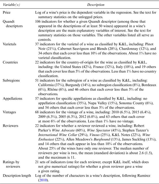
The other explanatory variables I include in the regression all serve as controls. The control variables hopefully ensure that any estimate of the effect of a descriptor on price is due to the descriptor itself or something non-obvious (rather than due to a correlation between the descriptor and something more obvious about the wine). I control for a wine's varietal, geographic origin, vintage year, reviewers, numerical ratings, and description length. See Table 1 for a summary of those controls and the other variables in my hedonic regression.
Variables in the Hedonic Regression

Notes: This table describes the variables included in the hedonic regression, which are all indicator variables, except the (log of the) price of a wine and length of its description. The percentages in parentheses are the frequencies with which an indicator variable occurs in the dataset. See the appendix for more details on the control variables.
B. Results and Discussion
Given a large number of explanatory variables and my focus on the Quandt descriptors, I do not report full regression results here, but they can be summarized as follows. When the previously discussed explanatory variables are included in the regression, there are 50,202 degrees of freedom left over from the 51,043 observations. About 67% of the variation in log prices is explained by those variables. The indicator variables for the 106 descriptors (which again are the Quandt descriptors that appear in the descriptions of at least 50 wines in my dataset) are jointly statistically significant (p-value < 0.01).
Despite their joint significance, many of the descriptors have effects that are not statistically significantly different from zero at conventional levels. Examples of descriptors with statistically insignificant effects include “silky” and “silky tannins.” The effect on a wine's price of “silky” appearing in its description is estimated to be only 0.4% (se = 0.6%, p-value = 0.49), where here and throughout I use Kennedy's (Reference Kennedy1981) and Van Garderen and Shah's (Reference Van Garderen and Shah2002) approach to estimating the effect of an indicator variable in log-linear regressions like Equation (1). The effect of “silky tannins” is 1.1% (se = 1.0%, p-value = 0.25), where I account for the fact that some descriptors such as “silky tannins” have other descriptors such as “silky” nested in them.
Some descriptors do have effects that are statistically different from zero. Of the 106 descriptors, 43 have effects that are significantly significant at the 10% level. Yet, some of those statistically significant effects are not substantively significant. For example, the effect of “velvety tannins” is statistically different from zero (p-value = 0.03), but it is arguably small at only 2.5% (se = 1.1%). A 2.5% change is less than a $1 change for any bottle under $40.
Some of the effects that are statistically different from zero are also neither statistically nor substantively different from the effects of other descriptors. The difference between having “velvety tannins” rather than “silky tannins” is estimated to be only about 1.4% (se = 1.4%) and not statistically different from zero (p-value = 0.32).
That result is noteworthy because it suggests an answer to Quandt's quandary. If given a choice between two wines that only differ in whether their tannins are described as silky or velvety, it seems consumers may have a slight preference for the wine with velvety tannins, but any preference is statistically indistinguishable from indifference. That finding would be supported by the fact that, according to Parker's wine glossary, “velvety” is a “textural description” and a “synonym for […] silky” (Wine Advocate, 2020). Velvety and silky tannins may indeed be synonymous for both wine critics and consumers.
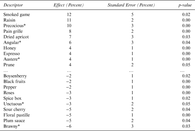
Although many of the Quandt descriptors have insignificant effects, some have effects that are significantly different from zero and each other. Table 2 summarizes the descriptors with effects that are statistically significant (at the 10% level, in particular) and the largest out of all the estimated effects (the 10 most negative and 10 most positive effects, in particular). As seen in that table, some descriptors such as “smoked game” are estimated as having a significant positive effect on the price, while others such as “brawny” are estimated as having a significant negative effect.
Hedonic Results for Descriptors with Most Significant Price Effects

Notes: This table reports, for the Quandt descriptors that have the most significant effects on price according to my hedonic regression, the estimated effect on the price of a wine (in percentage terms) of a descriptor appearing in the wine's description, the standard error of that estimated effect, and a p-value for a z-test of whether the effect is different from zero. These descriptors have the most significant effects in the sense that they are statistically different from zero at the 10% level and have one of the 10 most positive or negative effects. The descriptors are sorted by the size of their effect before rounding.
* Defined in Parker's wine glossary, as noted by Quandt (Reference Quandt2007, p. 133).
If those hedonic results are momentarily accepted, there is much to puzzle over. Why would consumers be willing to pay so much more for wine if an expert described it in terms of the smoked game? How much more or less would they be willing to pay if the expert described the game as being prepared differently, such as by roasting, steaming, or boiling? And what if the expert described the game as a specific type of animal such as a pheasant, boar, deer, squirrel, or some elusive or imaginary creature that few if any have tasted? Questions abound. The approach used earlier opens up some possibility of answering those questions, to the extent that relevant descriptors appear in wine descriptions, and to the extent that the results of such regressions are to be believed.
Unfortunately, my hedonic estimates are not necessarily to be believed. One potential issue is they may suffer from a reverse causality bias. It is widely recognized that a simple regression of wine prices on expert ratings may suffer from reverse causality because ratings may be a consequence and not just a cause of a wine's price (see, e.g., Oczkowski and Pawsey, Reference Oczkowski and Pawsey2019). My regression may suffer from an analogous issue because expert descriptions may be both a cause and consequence of a wine's price; Krumme (Reference Krumme2011), in particular, argues that a wine's price affects descriptions of it.
To try to address concerns about reverse causality, previous studies on wine prices and expert descriptions have used descriptions written based on “blind” tastings in which some information about wine such as its price and producer is masked from a taster, but the taster is given other information such as the wine's varietal, region, and vintage (Chen and McCluskey, Reference Chen and McCluskey2018, p. 391; Ramirez, Reference Ramirez2010, p. 144). That sort of “blind” tasting might minimize concern over prices affecting descriptions, but it would not eliminate the concern because the unmasked information could provide price signals to wine experts (Krumme, Reference Krumme2011). Prices and descriptions would be further entangled by any retasting of the sort described by Reuter (Reference Reuter2009) or any rewriting based on unmasked information.
If descriptions—even those written based on “blind” tastings—cannot be presumed to be only a cause and not also a consequence of price, then the literature on wine prices and expert ratings could perhaps suggest instrumental variables to use in a hedonic regression. Yet, at least for the dataset I have constructed, there are no obvious variables to use as instruments for the descriptors. Other methods such as the stated-preference survey discussed in Section IV or experimental methods like those suggested in the conclusion of this paper may be needed to estimate consumers’ MWTP for descriptors and thereby validate or invalidate my hedonic estimates.
Despite no obvious way to control for potential endogeneity, there are other possible issues with my hedonic estimates that can be addressed by applying a matching approach to the same dataset.
III. Matching Estimates
A. Data and Methods
Another potential issue with my hedonic regression is it ignored most of the rich text in the wine descriptions. Although some aspects of the wine descriptions were accounted for directly (most notably, the Quandt descriptors) and other aspects may have been accounted for indirectly through the control variables, most parts of the wine descriptions were ignored. If those ignored parts do not affect (or are not associated with) the price of a wine, then they can be safely ignored, but the premise of this paper is there might be a relationship between wine prices and descriptions.
The richness of wine descriptions makes it difficult to capture them in a simple regression. Including indicator variables for additional descriptors besides the Quandt descriptors would quickly exhaust the regression's degrees of freedom, so alternative approaches for quantitatively using rich text are needed.
The approach I adopt here is a text-matching estimator. Any matching estimator tries to match subjects who have received a treatment to control subjects who are as similar as possible, except they did not receive the treatment. After matching, the effect of the treatment on an outcome of interest can be estimated by comparing the outcomes of the matched subjects. Here, the “subjects” are wines, the “treatment” is whether a given Quandt descriptor appears in a wine's description, and the outcome of interest is the wine's price.
A text-matching estimator matches subjects based on rich texts associated with them. Mozer et al. (Reference Mozer, Miratrix, Kaufman and Anastasopoulos2020) compare different text-matching methods and recommend an approach I largely adopt. See the supplementary appendix to this paper for more details and discussion, but my approach was as follows. For each “treated” wine that has a given descriptor appear in its description and for each wine that was available as a possible “control” because the descriptor did not appear in its description, I created a simple representation of its description. Specifically, for a given wine, I represented its description as a one-dimensional array where the elements correspond to the unique words in any of the wines' descriptions, and each element took on the value of either unity or zero depending on whether the word appeared in the wine's description or not. That is a so-called “bag-of-words” representation of a text (Mozer et al., Reference Mozer, Miratrix, Kaufman and Anastasopoulos2020, p. 6). After doing that, I matched each treated wine to a control wine based on the similarity of the bag-of-words representations of their descriptions. Specifically, I matched them using one-to-one nearest neighbor matching without replacement (where Mozer et al., Reference Mozer, Miratrix, Kaufman and Anastasopoulos2020, also use one-to-one matching without replacement) based on the cosine similarity of their bag-of-words representations (where cosine similarity is the distance measure recommended by Mozer et al., Reference Mozer, Miratrix, Kaufman and Anastasopoulos2020). Each treated wine was in that sense matched to a control wine that is as similar as possible and ideally identical, except again that the descriptor of interest appears in the treated wine's description but not in the control wine’s description. Finally, I estimated the effect of the descriptor of interest on a wine's price as

where Pi(1) denotes the price of the i-th of N treated wines and Pi(0) denotes the price of the control wine matched to the i-th treated wine. The latter price serves as an estimate of what the price the i-th wine would have been if it had not been treated. Using the log difference between those prices implies the effect is (approximately) in percentage terms and thereby comparable to my earlier hedonic estimates. I apply that approach to the same dataset discussed above.Footnote 1
In addition to making greater use of the text in the wine descriptions, my matching approach addresses other potential issues with my hedonic regression. A log-linear form is a standard form to assume for hedonic regressions, but it might not be the most appropriate form. Even if it is, the explanatory variables could interact in more complicated ways than I assumed. My matching approach, in contrast, offers a nonparametric estimate of the descriptor's effect on (or association with) price.
Of note, there are other possible matching approaches besides the one I adopt. Exact matching (in which matched wines would be identical, except for one descriptor used to describe them) would be ideal, but exact matches are rare or non-existent in my dataset, especially if any attempt is made to account for the rich text in the wine descriptions. Propensity score matching (in which wines are matched based on estimated treatment probabilities) is another possibility, but at least for the logit regressions that conventionally underlie a propensity score matching approach, most of the text in the wine descriptions would need to be ignored to avoid exhausting the degrees of freedom for those regressions. Matching based on other representations of rich text (such as estimated topic probabilities from a topic model) is also possible, but again I have largely followed the approach advocated by Mozer et al. (Reference Mozer, Miratrix, Kaufman and Anastasopoulos2020).
B. Results and Discussion
The matching approach discussed previously is computationally intensive, and the similarity of matched subjects should be assessed, so here I focus on validating (or invalidating) a small number of results from my hedonic regression. I specifically focus on whether my matching approach suggests the descriptors “smoked game” and “brawny,” as well as “silky tannins” and “velvety tannins,” have effects that are similar to those suggested by my hedonic estimates. Recall that “smoked game” and “brawny” had the most significant positive and negative effects on price according to the hedonic estimates, while “velvety tannins” and “silky tannins” had little or no effect according to those estimates.
Consider first the appearance of “smoked game” as the treatment and the absence of that descriptor as the control. There are 55 wines in my dataset described by that descriptor, so the other 50,988 wines are available as possible matches. After applying the previously discussed matching approach, some matches were better than others. The highest cosine similarity between any matched treated and control wine was between—on the one hand—the 2013 Domaine Tollot-Beaut Corton-Bressandes Grand Cru with four reviews, including a Burghound review that said the wine had “notes of […] smoked game,” and—on the other hand—the same wine listed under a different stock-keeping unit (SKU) and including all of the same reviews, except the Burghound review. Because they differ in terms of their SKUs and the Burghound review, I did not ignore one of those two wines as a duplicate of the other when constructing my dataset, but my matching approach found two wines that are identical except for one review.Footnote 2
The cosine similarity for that match was 0.85, which is relatively high. The highest possible value is unity, which would occur if two descriptions had the exact same text. The lowest possible value is zero, which would occur if two descriptions had no text in common.
Not all matches were that similar. The mean of the cosine similarities between the matched wines was 0.49 (se = 0.08). The matched wines were nevertheless as similar as possible in terms of the cosine similarity of bag-of-words representations of their descriptions.
The matches were also similar in terms of many of the variables used as controls in my earlier hedonic regression, even though my matching approach was strictly in terms of the text of the wine descriptions and not directly in terms of those variables. Comparing each treated wine to its matched control wine, 82% of the matched wines were the same in terms of their varietal as classified by K&L. Similarly large percentages of the matched wines (ranging from 76% to 100%) were the same in terms of their geographic origin and whether or not they were reviewed by a given reviewer. The matched wines also had similar description lengths; the length of a treated wine's description was about 97% of the length of its matched control wine's description on average (se = 31%).
The matched wines were less similar in terms of their vintage year and numerical ratings. In terms of vintage: Only about 38% shared the same vintage. Dissimilarity along that dimension could be due to poor matching, although it is not implausible that better matches might be found across years (e.g., between the same producer) rather than within years. In terms of ratings: The proportion of matched wines with the same rating from a given reviewer varied but was generally low. To give one example, for each of the 40 treated wines with a numerical rating from Parker, only 14 of the matched control wines had the same rating from him.
The matching is not exact, but again, the matches are as similar as possible. For brevity, it can be noted that the match quality for each of the other treatments discussed later was very similar to the match quality for the “smoked game” treatment. The mean cosine similarities were 0.50 or near that. The vast majority of the matched wines were the same in terms of their varietal, geographic origin, and whether a given reviewer reviewed the wine. Their description lengths were also close to one-to-one on average. The matches were less similar in terms of their vintage and ratings.
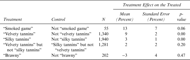
After matching, the effect of the appearance of the “smoked game” treatment can be estimated using Equation (2). Its estimated effect is reported in Table 3 along with the effects of the other treatments discussed later. Its effect is estimated to be about 13% (se = 7%, p-value = 0.06). That matching estimate is similar to my earlier hedonic estimate in terms of its substantive and statistical significance.
Matching Results for Price Effects of Select Descriptors

Notes: This table reports my matching estimates of the effect on the price of a wine of a given “treatment” relative to a given “control,” where the treatments and controls relate to the appearance or absence of a descriptor in a wine's description. The mean price effect, its standard error, and a p-value for a Welch's t-test of whether the effect is different from zero are reported. The number of treated wines (N) is also reported. See the text for a discussion of the treatments and match quality.
Next, consider “brawny” as the treatment and the lack of that descriptor as the control. Its effect is estimated to be negative but small (at about half the size of my earlier hedonic estimate) and not statistically different from zero (p-value = 0.47). That matching estimate is not necessarily inconsistent with my earlier hedonic estimate because of the uncertainty associated with those estimates. Yet unlike my hedonic approach that suggested brawny had a relatively large negative effect on the price, my matching approach suggests that descriptor has little or no effect.
“Velvety tannins” was a descriptor with a relatively small but statistically significant effect according to my hedonic estimates. If its appearance is taken as the treatment and its absence as the control, then my matching estimate of its effect is 9.5% (se = 1.5%, p-value < 0.01), which is bigger than my hedonic estimate.
“Silky tannins” was a descriptor with an insignificant effect according to my hedonic estimates. If that descriptor's appearance is now taken as the treatment and its absence as the control, then my matching estimate of its effect is 3.5% (se = 1.2%, p-value < 0.01), which is slightly bigger than but not necessarily inconsistent with my hedonic estimate.
My matching estimates are therefore generally consistent or not inconsistent with my hedonic estimates. The matching estimates, however, have their own potential issues too. The richness of wine descriptions means that matching will always be inexact, which means that matched wines will always differ in other ways besides the descriptor of interest, which in turn means that matching estimates of the effect of a descriptor could be conflated with the effects of other descriptors. If “velvety tannins” and “silky tannins” have their own separate effects on the price of wine but tend to co-occur together, for example, then the matching estimates could conflate the effect of those descriptors.
To more directly examine the relative effects of different descriptors, different treatment and control conditions can be considered. The relative effects of velvety and silky tannins are of particular interest because of Quandt's quandary. There are 1,281 wines in my dataset for which the “velvety tannins” descriptor appears and the “silky tannins” descriptor is absent. Those wines with velvety but not silky tannins can be taken as treated wines. Each of those wines can be matched to one of the wines for which the “velvety tannins” descriptor is absent and the “silky tannins” descriptor appears. The effect of having velvety rather than silky tannins is then estimated to be 2.4% (se = 1.8%) and not statistically different from zero (p-value = 0.20). My matching approach, therefore, suggests the same answer to Quandt's quandary as to my hedonic approach: Consumers may have a slight preference for velvety over silky tannins, but any preference is statistically indistinguishable from indifference. My matching estimate, as well as the hedonic estimate of that effect, could nevertheless still be confounded with the effects of other descriptors.
Other potential issues with my matching approach include the previously discussed endogeneity issue from which my hedonic approach may suffer. Both approaches may also fail to account for important determinants of a wine's price; the price of a given vintage of a wine may be affected by descriptions of previous vintages of that wine, for example, as Ramirez (Reference Ramirez2010) argues.Footnote 3 Lacking easy or obvious ways to address such issues, other approaches may be needed.
IV. Stated Preference Survey
A. Questions and Sample
My third approach for trying to estimate MWTP for the Quandt descriptors was a stated-preference survey of U.S. wine consumers. The entire survey is discussed in the supplementary appendix, but the key questions I will focus on here are as follows.
After obtaining their informed consent at the start of the survey, I asked respondents to self-report their knowledge of wine (on a five-item Likert scale with “Average” as the center option), to read a “cheap talk” script of the sort that has been shown to mitigate hypothetical bias (Penn and Hu, Reference Penn and Hu2019), and to report the price they “typically” pay when shopping for a bottle of wine (where the options for that were “$5,” “$10,” “$20,” “$30,” “$40,” “$50,” or an open-ended option of “Over $50” that required them to specify a dollar amount over $50).
I then asked respondents which of two wines in their “typical price range” they would buy if the wines were “almost identical,” except each wine had a different descriptor associated with it. I asked: “Suppose that, while shopping for wine, you find two wines in your typical price range. The wines are almost identical, except one is described as having silky tannins and the other is described as having velvety tannins. Which wine would you buy?” I thereby asked respondents essentially the same question that Quandt asked rhetorically in his article. The four choices available to respondents were: “The wine with silky tannins,” “The wine with velvety tannins,” “Either of those wines,” and “Neither of those wines.”
Respondents who chose “Either of those wines” were subsequently asked which wine would they buy if they were forced to choose. A forced-choice follow-up question seemed appropriate, given that trying to choose between wines described by descriptors such as silky and velvety tannins may be difficult and given that any preference for one over the other might be slight. It is of interest to know whether respondents who say they would buy either wine are truly indifferent; if they are, they should break evenly between the two wines when forced to choose.
Respondents who chose “Neither of those wines” were also asked the forced-choice question so they followed the same path as other respondents, but in the analysis below, I ignore their responses to such questions, given that they said they would not buy either wine.Footnote 4
After expressing their preference between the two wines, respondents were directly asked about their MWTP in dollar terms for the wine they said they preferred relative to the other wine. Respondents who said they would buy the wine with, say, velvety rather than silky tannins were asked: “You said you'd buy the wine with velvety tannins. What's the most you'd be willing to pay for that wine, compared to the almost identical wine with silky tannins?” A similar question was asked of respondents who said they would buy the wine with silky rather than velvety tannins.
Asking each respondent which wine they prefer and then asking them to report a non-negative MWTP for it was inspired by Hanley et al. (Reference Hanley, Colombo, Kriström and Watson2009). Their study assumes different people may have a positive, zero, or negative MWTP for a given change. Here, people could have a positive MWTP for a wine with velvety rather than silky tannins, zero MWTP for that, or a negative MWTP for that in the sense they prefer a wine with silky rather than velvety tannins. Hanley et al. (Reference Hanley, Colombo, Kriström and Watson2009) ask respondents about their preferred change, then ask respondents to report a non-negative MWTP for their preferred change, and finally, estimate average MWTP across all respondents for a given change by assuming that the negative of a respondent's MWTP for their preferred change is equal to their negative MWTP for the change they do not prefer. I make the same assumption later to estimate the average MWTP for one wine rather than the other. See Hanley et al. (Reference Hanley, Colombo, Kriström and Watson2009, sec. 4) for a defense of their approach over other possible approaches (such as ignoring respondents who do not prefer a given change or asking those respondents about their willingness to accept compensation).
When respondents to my survey expressed their MWTP, the options available to them were: “At most zero dollars more,” “At most one dollar more,” “At most 5 dollars more,” “At most 10 dollars more,” and an open-ended option of “Over 10 dollars more” that required respondents to specify an amount above 10 dollars. The options I presented to respondents were loosely based on the size of the previously discussed estimates and the expectation that most people would typically pay less than $50 for a bottle of wine. The options were also based on the desire to include $0, as well as a small non-zero amount (such as $1), as choices. If a respondent is indifferent between the two wines, their MWTP should be $0. If a respondent has a slight preference, they should be willing to pay a slightly different amount.
Ideally, I would have asked respondents about their MWTP for many other descriptors besides silky or velvety tannins, but there are practical limits to doing that, so I only asked about a few descriptors. Asking about only a few can still yield insight. If my survey suggests that consumers’ MWTP for velvety rather than silky tannins is similar to my hedonic and matching estimates, then that complementary evidence reinforces the conclusions drawn.
Other questions in my survey included attention checks toward the beginning and end of the survey. Two questions from Aqueveque's (Reference Aqueveque2018) test of wine knowledge were also asked toward the end of the survey. One question was about the meaning of tannins, and the other was about common descriptors for a certain grape varietal.
After my survey was approved in accordance with my university's policies for human subjects research, I purchased 500 responses through SurveyMonkey, which is a publicly-traded company that maintains a panel of U.S. participants who voluntarily take part in online surveys. Participants complete surveys in return for small credits toward a gift card (typically 50¢), small chances at winning a $100 gift card, or small charitable donations. SurveyMonkey also allows targeting subpopulations, including respondents who purchased wine in the last 30 days; I targeted that subpopulation so my respondents can be assumed to be wine consumers.
By all indications, SurveyMonkey is a reliable source from which to collect responses. Bentley et al. (Reference Bentley, O'Neill, Quehl and Lottridge2020) obtained responses to the same questions from several different survey companies and found SurveyMonkey to offer results as reliable as more expensive alternatives (ibid., p. 9).
B. Results and Discussion
In total, 501 completed responses from U.S. wine consumers were provided by the survey company. The company also provided 70 incomplete responses from people who started the survey by answering at least the first question but did not finish; I ignored those responses because they apparently withdrew their consent to participate. Given the number of complete and incomplete responses, my survey's completion rate is about 88%, which is higher than might be expected based on the potentially maddening nature of some of the questions.
Among the 501 respondents who completed the survey, 469, or about 94%, passed the attention checks. I ignored all respondents who did not pass the attention checks.
Wine experts may have different perceptions or preferences than novices, especially when it comes to wine descriptions (Ashton, Reference Ashton2017, sec. 3.B; Marks, Reference Marks2015; Storchmann, Reference Storchmann2012, sec. 6.B.), so in addition to pooling all 469 respondents, I split my sample into experts and non-experts. I classify respondents as “experts” if they self-reported at least an average level of knowledge and also correctly answered the questions I asked from Aqueveque's (Reference Aqueveque2018) test. There are 103 such respondents in my sample. I classify everyone else as “non-experts.”
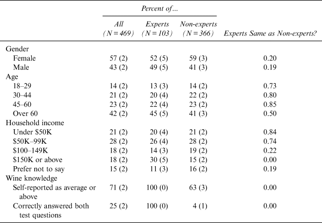
Demographic information on my sample is reported in Table 4. The sample is perhaps more female, older, and rich than the U.S. population, but that may be representative of U.S. wine consumers. The experts and non-experts differ in their wine knowledge by construction, and they seem to be somewhat richer, but they are otherwise similar in terms of their demographics.
Demographic Information on Survey Respondents

Notes: This table shows the proportion of my survey respondents who fall into a given demographic category. Standard errors are reported in parentheses. Those proportions are also broken down by whether a respondent was an “expert” (i.e., self-reported at least an average level of wine knowledge and correctly answered both wine knowledge test questions) or “non-expert” (i.e., everyone else). To assess whether there are any differences between experts and non-experts, the p-values for z-tests of independent proportions are reported in the last column. Of note, the correlation between respondents’ self-reported wine knowledge and their score on that wine knowledge test was 0.36 (p-value < 0.01).
In terms of the prices that respondents typically pay when shopping for a bottle of wine, the mean (standard deviation) was about $14 ($8). Experts reported paying slightly more on average than non-experts, but the difference was less than $1 (specifically, 68¢) and not statistically different from zero (based on a Welch's t-test; p-value = 0.38). Only one respondent reported typically paying over $40; that respondent was an expert who said they typically pay $100 for a bottle of wine.
When respondents were asked whether they would prefer the wine with silky or velvety tannins, some respondents said they would prefer neither wine. About 10% of the 469 respondents, as well as about 10% of both experts and non-experts, said that (with standard errors of about 1%, 3%, and 2%, respectively). There was no statistically significant difference between the percentage of experts and non-experts who said they would prefer neither wine (based on a z-test of independent proportions; p-value = 0.97).
Almost exactly 50% (se = 2%) of the respondents initially said they preferred either wine. When forced to choose, 52% (se = 3%) of those respondents chose the wine with silky rather than velvety tannins, which is close to half of them and not statistically different from it (p-value = 0.51). The fact that those respondents broke almost evenly between the wines when forced to choose suggests they were indeed indifferent.
Among the roughly 40% of respondents who were not forced to choose because they initially said they preferred one wine over the other, about 53% (se = 4%) said they preferred the wine with velvety rather than silky tannins, which is close to 50% and not statistically different from it (p-value = 0.38).
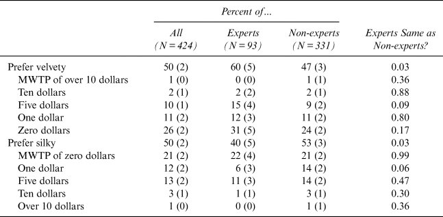
Table 5 summarizes the preferences expressed by the respondents, including the forced choices of respondents who initially said they preferred either wine and excluding respondents who said they preferred neither wine. As shown in that table, there was an even split between the wines with velvety and silky tannins among the respondents as a whole.
Survey Results for Wine Preferences

Notes: This table reports, for all survey respondents except the 45 who said they preferred neither wine, the percentage who said they preferred the wine with velvety or silky tannins. The forced choices of the 234 respondents who initially said they would prefer either wine are included in the calculations. The table also shows their MWTP for their preferred wine relative to the other wine. Standard errors are reported in parentheses. Responses are also broken down by whether a respondent was an “expert” or not. To assess whether there are any differences between experts and non-experts, the p-values for z-tests of independent proportions are reported in the last column.
Experts and non-experts did choose somewhat differently, however, as shown in the same table. About 60% of experts chose the wine with velvety rather than silky tannins, which is statistically different from half of them (p-value = 0.04), and also statistically different from the 47% of non-experts who chose the same (p-value = 0.03), which itself is not statistically different from one-half (p-value = 0.35). Thus, unlike the non-experts, the experts leaned slightly toward the descriptor that may have a slight premium according to the hedonic and matching estimates.
Table 5 also summarizes respondents’ MWTP in dollar terms for their preferred wine relative to the other wine. For all the respondents, the experts, and the non-experts who preferred velvety over silky tannins, the mode of their MWTP for their preferred wine was $0. The same is true for those who preferred silky over velvety tannins.
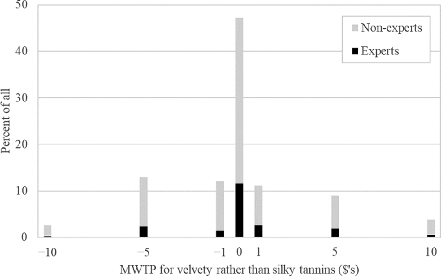
Figure 1 shows the distribution of MWTP for velvety rather than silky tannins among all the respondents, where I follow Hanley et al. (Reference Hanley, Colombo, Kriström and Watson2009) by assuming that the negative of a respondent's MWTP for silky rather than velvety tannins is their negative MWTP for velvety rather than silky tannins. As that figure suggests, a near or slight majority of all respondents, experts, and non-experts said they would pay exactly $0 (specifically, 47%, 53%, and 46% of those groups said that). Over two-thirds of each of those groups had a MWTP within $1 of $0.
Distribution of MWTP for a Wine with Velvety Rather Than Silky Tannins
Notes: This figure shows, for all survey respondents (except the 45 who said they preferred neither wine), a histogram of respondents’ MWTP for a wine with velvety rather than silky tannins. A negative MWTP denotes a MWTP for silky rather than velvety tannins. Whether respondents were experts or non-experts is also shown. Six outliers in MWTP (three less than −$10 and three more than $10) lie beyond the range shown above, as discussed in the text.

My survey, therefore, suggests most consumers have a zero or near-zero MWTP for velvety rather than silky tannins; that would be consistent with “velvety” and “silky” being synonyms and not inconsistent with my hedonic and matching estimates that suggested at most a small price premium for velvety over silky tannins.
Yet, not all respondents had a near-zero MWTP. Indeed, there were even a few outliers that lie beyond the range shown in Figure 1. Three respondents, who were all non-experts, reported MWTP for silky rather than velvety tannins of $20, $20, and $14. Three more respondents, who were also all non-experts, reported marginal willingnesses to pay for velvety rather than silky tannins of $14, $25, and $50. Those dollar amounts seem suspiciously large (perhaps because those six respondents confused the total cost of wine with its marginal cost relative to the other wine), but there were other non-zero valuations too.
Despite some non-zero valuations, the average MWTP is essentially $0. As a simple average across respondents, the mean MWTP for velvety rather than silky tannins is negative 8¢ for all respondents, positive 38¢ for experts, and negative 21¢ for non-experts (with standard errors of 22¢, 33¢, and 27¢). None of those amounts are statistically different from zero (with p-values of 0.72, 0.25, and 0.44). That the mean difference in MWTP between experts and non-experts suggests a slight difference of opinion, although the difference is only 58¢ and not statistically different from zero (p-value = 0.17).
To more directly compare the survey estimates of mean MWTP to my hedonic and matching estimates, a respondent's MWTP can also be expressed in percentage terms relative to the price they reported typically paying for a bottle of wine. Table 6 recalculates the mean MWTP in those terms.
Survey Results for Mean MWTP in Percentage Terms

Notes: This table reports the means (and standard errors) of respondents’ MWTP in percentage terms for a wine with velvety rather than silky tannins (except the 45 who preferred neither of those). Responses are also broken down by whether a respondent was an expert or not. The p-value for a Welch's t-test of whether the mean MWTP of experts is different from the mean MWTP of non-experts is reported in the last column. A respondent's MWTP in percentage terms was calculated as their MWTP in dollar terms for their preferred descriptor, on the one hand, all over the price in dollars they said they typically pay for a bottle of wine, on the other hand. A negative MWTP was again used to denote a MWTP for silky rather than velvety tannins.
As reported in the table, the mean MWTP in percentage terms for velvety rather than silky tannins is about negative 2% (se = 2%) for all respondents, which is not statistically different from zero (p-value = 0.28). That zero or near-zero survey estimate does not seem too inconsistent with my hedonic and matching estimates of at most a small premium for velvety rather than silky tannins.
Interestingly, the mean MWTP over all respondents may be masking a difference of opinion between experts and non-experts. Experts have a mean MWTP of about positive 3% (se = 3%) while non-experts have a mean MWTP of negative 3% (se = 2%). Neither of those means are statistically different from zero at conventional levels (with p-values of 0.22 and 0.11), but the mean difference between them is statistically significant (p-value = 0.05). That finding could be consistent with a slight premium for velvety rather than silky tannins if the preferences of experts matter more to price determination.
V. Conclusions
This paper tried to estimate wine consumers’ MWTP for wines described by the specific descriptors that Quandt deemed to be bullshit. If consumers are unwilling to pay, then those descriptors are not necessarily false, but consumers treat them as valueless. If consumers are willing to pay, then the descriptors are not necessarily true, but consumers apparently value them.
Three approaches to estimate consumers’ MWTP for the Quandt descriptors were used: a simple hedonic regression, a text-matching estimator, and a stated-preference survey. Each approach has potential issues, but overall, they suggested two main conclusions.
One conclusion is that most consumers seem to have little if any MWTP for wines described by most of the Quandt descriptors. My hedonic approach suggested the majority of the descriptors have a price premium of zero or near-zero. My matching and survey estimates were generally consistent or not inconsistent with my hedonic estimates, at least for the select descriptors considered.
The other conclusion is that some consumers have a non-zero MWTP for wines described by some of the Quandt descriptors. The hedonic approach suggested some descriptors have price premiums (or discounts) that are significant in the statistical sense and arguably significant in the substantive sense. My matching approach suggested the same. And my survey approach suggested some expert and novice wine consumers are willing to pay more than nothing for some descriptors.
If some consumers do have a non-zero MWTP for wines described by some of the Quandt descriptors, then the question becomes: What exactly are they paying for? If they are paying for aspects of a wine that can be objectively verified (perhaps through the sort of chemical analysis that underlies Barth et al.'s Reference Barth, Katumullage, Yang and Cao2021 study), then the Quandt descriptors would seem to be much less bullshitty than he suggested. If consumers are paying for a wholly subjective effect, then Quandt may still be justified in deeming the descriptors bullshit. Experiments similar to those conducted by Goldstein (Reference Goldstein2019) may help determine whether people are paying for real or imaginary aspects. An investigator could identify a wine that an expert has described as having both “silky tannins” and “velvety tannins” (such as the 2010 Chateau Haut-Bailly that James Suckling described as having both). A subject could be given two masked samples of that same wine. The investigator could truthfully tell the subject that a wine expert has described the wine in the first sample as having “silky tannins” and the wine in the second sample as having “velvety tannins.” If a subject is not indifferent between those two samples of the same wine, then their preference could only be due to a wholly subjective effect of the different descriptors.
Supplementary Material
To view supplementary material for this article, please visit https://doi.org/10.1017/jwe.2021.24.