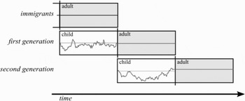
In this paper, we use mathematical modeling to evaluate Trudgill's theory of new-dialect formation, as applied to the emergence of New Zealand English (Trudgill, Reference Trudgill2004; see also Gordon, Campbell, Hay, Maclagan, Sudbury, & Trudgill, Reference Gordon, Campbell, Hay, Maclagan, Sudbury and Trudgill2004; Trudgill, Reference Trudgill1986; Trudgill et al., Reference Trudgill, Gordon, Lewis and Maclagan2000). Our goals are twofold. The first is to investigate certain properties of the propagation of language change. Trudgill's theory of new-dialect formation for isolated speech communities has an interesting and theoretically controversial property, which Trudgill calls determinism. There is no role for social factors such as prestige or identity in the emergence of isolated new dialects such as New Zealand English. Instead, new-dialect formation is purely frequency-based, in terms of exposure to tokens of language use by the speakers with whom one interacts. That is, the primary or sole social factor involved in new-dialect formation is accommodation (Giles, Reference Giles1973). Trudgill even questioned whether accommodation is “social” in the sense of behavior potentially under the control of human beings in social interaction. He argued that accommodation is universal (Trudgill, Reference Trudgill1986:2), and more recently, he suggested that accommodation has an innate biological basis (Trudgill, Reference Trudgill2004:28; Reference Trudgill2008:252).

Trudgill's theory is related to usage-based theories of linguistic knowledge and language use (e.g., Bybee, Reference Bybee2001; Pierrehumbert, Reference Pierrehumbert, Boc, Hay and Jannedy2003) in that linguistic behavior is determined by language use in communicative interaction. Trudgill's deterministic theory corresponds to a neutral evolution model in evolutionary theory, as we will argue later. Trudgill's theory contrasts with “classical” sociohistorical linguistic theory, in which variants of linguistic variables are associated with social factors (Labov, Reference Labov1972): this association is part of speakers' knowledge about their language, and propagation of language change is the result of the relationship between speakers and those social factors. There are debates about what those social factors are (e.g., social class, [covert] prestige, group identity), and how speakers relate to them in propagating certain linguistic variants at the expense of others. What matters in Trudgill's theory, however, is that no such factors are associated with linguistic variants; frequency of use and accommodation are the sole mechanisms necessary to account for new-dialect formation.

The classical sociohistorical linguistic theory corresponds to a selection model of change by replication, in which individual variants have an associated “fitness” value, as we argue later. Thus our evaluation of Trudgill's theory is a test of whether a neutral evolution model can be a complete model of the propagation of language change in an isolated new-dialect formation situation.

Our second goal is to bring mathematical models to bear on the explanation of empirical observations of language change, and thereby enrich sociohistorical linguistic theory. Mathematical models have been used to model numerous aspects of social behavior. For example, although the motion of an individual may not be predictable, the motion of groups of individuals might have statistical aspects that have some degree of regularity. This has been used to model the motion of people down corridors and in the formation of trails in open spaces (Helbing, Molnár, Farkas, & Bolay, Reference Helbing, Molnar, Farkas and Vicsek2001; Schreckenberg & Sharma, Reference Schreckenberg and Sharma2001). This is of particular importance in the understanding of the way people move through restricted exits, where overcrowding can lead to potentially lethal crushes and stampedes (Helbing, Farkas, & Vicsek, Reference Helbing, Farkas and Vicsek2000; Kirchner & Schadschneider, Reference Kirchner and Schadschneider2002). Such considerations have also been used to reduce the risk of dangerous overcrowding at large outdoor events (Batty, Desyllas, & Duxbury, Reference Batty, Desyllas and Duxbury2003). Regularities in the flow of traffic may, in the same way, also be amenable to analysis. Computational models of traffic flow based on a similar approach (Helbing, Reference Helbing2001) have the potential to yield useful traffic forecasts and to plan new road networks (Kerner, Reference Kerner2002; Maerivoet & De Moor, Reference Maerivoet and De Moor2005).

The implementation of theories, particularly quantitative theories such as those found in sociohistorical linguistics, through mathematical models is essential for evaluating their plausibility as well as their utility. Such models are essentially probabilistic. That is, they predict or simulate overall behavioral patterns of the collectivity rather than predicting the occurrence of individual events. It is a commonplace in historical linguistics that particular events of language change cannot be predicted (e.g., Trudgill, Reference Trudgill2004:26–27). Trudgill et al. specifically describe their “deterministic” model as probabilistic, in that the “deterministic” theory predicts the overall proportions of variants used by speakers, not the particular proportion of variants used by any individual speaker (Trudgill et al., Reference Trudgill, Gordon, Lewis and Maclagan2000:310).

We begin by outlining what is known about the basic facts surrounding the emergence of New Zealand English, and Trudgill's theory of new-dialect formation as he applies it to this situation. We discuss some of the potential empirical difficulties in applying Trudgill's theory to New Zealand English (many of which are also raised in Kerswill, Reference Kerswill2007). However, the focus of our paper is on whether Trudgill's theory can account for what Trudgill predicted, even if there is doubt as to whether Trudgill's predictions actually hold for New Zealand English.

We then turn to the modeling of Trudgill's theory. The mathematical model presented in this paper is based on the usage-based theory of language change proposed by Croft (Reference Croft2000), who is also cited by Trudgill in support of his deterministic theory (Trudgill, Reference Trudgill2004:150–151). This model is essentially an evolutionary one, which fits well with both a usage-based theory of innovation and the sociohistorical linguistic theory of propagation of innovations in a speech community (Croft, Reference Croft2000, Reference Croft and Thomsen2006). We explore a variety of neutral evolution models that represent the essential characteristics of Trudgill's deterministic theory of new-dialect formation, in particular the essential role of accommodation in Trudgill's theory, and describe their properties with respect to theories of language change.

We conclude, among other things, that none of the neutral evolution models we explore can account for the New Zealand English data under plausible assumptions. This is not to say that neutral evolution plays no role in new-dialect formation, or other circumstances of language change, for that matter. In fact, Trudgill's explanation for the central fact of the emergence of New Zealand English—that on the whole, the variant used by the majority of speakers emerges as the variant of the new dialect—is confirmed by our model. However, our model also implies that new-dialect formation, like other sociolinguistic situations of language change, requires a selection mechanism of some sort in addition to the neutral-evolution mechanisms advocated by Trudgill.

THE CREATION OF NEW ZEALAND ENGLISH: DEMOGRAPHY AND LANGUAGE

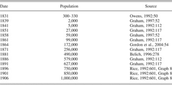
A crucial aspect of Trudgill's theory for the emergence of isolated new dialects is demography. If the result is determined by the proportions of variants in the input provided by the immigrants and their accommodation in communicative interaction, one must gather as much information as possible about the input. New Zealand English is one of the most recent varieties of colonial English to emerge. Although the first European settlers arrived in the 1790s, it was not until the Treaty of Waitangi was signed in 1840 that substantial numbers of Europeans began to arrive in New Zealand (Gordon et al., Reference Gordon, Campbell, Hay, Maclagan, Sudbury and Trudgill2004:38–39; Trudgill, Reference Trudgill2004:24). The European population increased dramatically from 1850 to around 1890, as indicated in the figures in Table 1.

Table 1.

European population of New Zealand in the nineteenth century

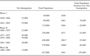
Between 1831 and 1881, 400,000 persons migrated to New Zealand; of these, 300,000 stayed in New Zealand. During the same period, 250,000 persons were born in New Zealand (Belich, Reference Belich1996:278). More precise figures for immigration between 1858 and 1890 are given by Graham (Reference Graham and Rice1992:125), and are compared in Table 2 with the population figures from Table 1 (the figures in italics at the right represent the approximate number of native-born New Zealanders from the preceding date; however, it understates the native-born because it does not include deaths since the preceding date).

Table 2.

A comparison of immigration to total population in New Zealand, 1858–1890

*250,000 native-born inhabitants in 1881 (Belich, Reference Belich1996:278).

†300,000 native-born inhabitants in 1886 (Graham, Reference Graham and Rice1992:112).

Table 2 indicates three phases of demographic change in nineteenth-century New Zealand. Phase I, from the 1840s to around 1864, was a period when almost all the European population increase in New Zealand was by immigration. Phase II, from 1864 to around 1886, was the period when the first substantial New Zealand native generation was born; significant immigration continued through Phase II. Phase III, from 1886 until after 1900, was a period when immigration, or at least net immigration, largely ceased. Immigration did not pick up significantly again until after 1900;Footnote ¹ but by then, net new immigration was only a small percentage of the total population (McKinnon, Reference McKinnon1997:49). Native-born New Zealanders constituted around 48% of the total population in 1881, 52% in 1886, and 60% in 1901 (Hamer, Reference Hamer and Sinclair1997:144).

The vast majority of immigrants at this time came from the British Isles (Gordon et al., Reference Gordon, Campbell, Hay, Maclagan, Sudbury and Trudgill2004:44), although many of these came via Australia. The British immigrants largely came from southern England (Gordon et al., Reference Gordon, Campbell, Hay, Maclagan, Sudbury and Trudgill2004:139; Trudgill, Reference Trudgill2004:16), Scotland, and Ireland; the approximate proportion was 50% English, 27% Scottish, and 23% Irish (Trudgill, Reference Trudgill2004:13, 16, citing McKinnon, Reference McKinnon1997). There were attempts to exclude or restrict Irish Catholic immigrants, but they were largely unsuccessful (Gordon et al., Reference Gordon, Campbell, Hay, Maclagan, Sudbury and Trudgill2004:42, 43). Thus, a variety of British English dialects, though not northern English dialects, contributed to the formation of New Zealand English.

A distinctive, relatively stable New Zealand English dialect emerged with the generation of New Zealanders born around 1890 (Trudgill, Reference Trudgill2004:24–25, 113). This is approximately the second generation of native-born New Zealanders. Remarkably, there are recordings available of some of the first generation of native New Zealand speakers, that is, those born from the 1850s to the 1880s. In the late 1940s, the New Zealand National Broadcasting Service sent a Mobile Disc Recording Unit to record music and oral histories from towns and rural settlements (Gordon et al., Reference Gordon, Campbell, Hay, Maclagan, Sudbury and Trudgill2004:1–4). These speakers represent a generation before the emergence of the New Zealand English variety, albeit a biased sample—for example, speakers from larger towns and cities were not interviewed, and a larger number of male speakers and speakers from the South Island were interviewed.

These recordings were purchased and used to analyze the origins of this colonial variety in the Origins of New Zealand English (ONZE) project.Footnote ² The major report of this study is the book by Gordon et al. (Reference Gordon, Campbell, Hay, Maclagan, Sudbury and Trudgill2004). The deterministic theory was originally proposed by Trudgill in his 1986 book on dialects in contact (Trudgill, Reference Trudgill1986). Trudgill was part of the ONZE project team; the team applied the deterministic theory to New Zealand English in Trudgill et al. (Reference Trudgill, Gordon, Lewis and Maclagan2000). Trudgill published a slightly different version of his theory in a separate book (2004); see also Trudgill (Reference Trudgill2008). We now turn to Trudgill's theory, chiefly as it is presented in Trudgill (Reference Trudgill2004).

TRUDGILL'S DETERMINISTIC THEORY

Trudgill's deterministic theory is intended to apply only to a very specific type of language change: new-dialect formation as a result of dialect mixture in a community isolated from other speakers of the same language (what Trudgill calls a “tabula rasa” situation [Trudgill, Reference Trudgill2004:26]). Thus, for example, it does not cover the new town koinés of towns such as Milton Keynes in England (Kerswill, Reference Kerswill1996; Kerswill & Williams, Reference Kerswill and Williams2000, Reference Kerswill and Williams2005), which is surrounded by older English-speaking communities, let alone language change in established speech communities. New Zealand English appears to satisfy these criteria. New Zealand was overwhelmingly populated by speakers of English varieties, and the influence of the indigenous language, Maori, was minimal (Gordon et al., Reference Gordon, Campbell, Hay, Maclagan, Sudbury and Trudgill2004:69–70, 219; Trudgill, Reference Trudgill2004:4–5). However, New Zealand was populated by speakers of different English varieties, leading to dialect mixture. New Zealand is geographically isolated from other English-speaking communities, both the United Kingdom and Australia, although there was significant movement between New Zealand and Australia (Gordon et al., Reference Gordon, Campbell, Hay, Maclagan, Sudbury and Trudgill2004:224–230). Finally, the creation of a new speech community eventually led to the creation of a new English dialect, New Zealand English. Trudgill argued that the process of new-dialect formation, at least in this type of situation, takes two generations, or approximately fifty years (Trudgill, Reference Trudgill2004:23).

Trudgill's theory involves several different mechanisms, but the central hypothesis is that, within certain bounds, the outcome of the new-dialect formation process can be predicted using a small number of principles, if one knows the linguistic variants of the input dialects and the proportions of immigrants speaking those dialects. The basic proportions of immigrants speaking the broad dialects of southern England, Scotland, and Ireland were given earlier, and a large part of Trudgill's book is devoted to identifying the linguistic variants of the input dialects in mid- to late-nineteenth-century Britain (Trudgill, Reference Trudgill2004:31–82). The most important principle of Trudgill's theory is that the most frequent variant, based on demography, survives to form part of the new dialect.

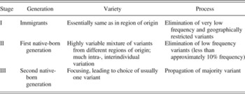
Trudgill divided the process of new-dialect formation into three stages, corresponding roughly to three discrete generations of speakers. Stage I represents the immigrant generation: native speakers of different British dialects who arrived in New Zealand after the middle of the nineteenth century. This generation basically speaks the dialect of their place of origin. However, in the dialect contact situation of early colonial New Zealand, Trudgill argued that variants that are in a very small minority or are geographically very restricted will be eliminated even at this early stage, giving plausible examples from a number of colonial dialects (his “rudimentary leveling” [Trudgill, Reference Trudgill2004:89–93]). Trudgill also suggested that interdialect forms may arise in Stage I (ibid., 94–99). Stage I corresponds basically to Phase I of the demographic history of New Zealand described earlier. A small number of Phase I speakers were recorded by the Mobile Disc Recording Unit.

Stage II represents the first native-born generation; this is the generation chiefly recorded by the Mobile Disc Recording Unit. The availability of these recordings allows us to observe the features of a transitional generation that has been lost to linguistic analysis in other new-dialect formation situations (Trudgill, Reference Trudgill2004:100). Trudgill argued that Stage II is characterized in the ONZE project data by extreme variability, both in comparison to the source dialects in Britain and in comparison to speakers of the second native-born generation. Trudgill argued that children in this generation do not have a societal norm among their peers because of the absence of such norms in the new-dialect situation. Hence “in diffuse dialect-contact situations the role of adults will be more significant than is usually the case” (ibid., 101). Because the adults came from a variety of dialect backgrounds, the children's language will contain a mixture of variants originally from different dialect areas in Britain. Trudgill gave the example of a Stage II ONZE speaker, Mrs. German, whose parents were from Suffolk, but lived in a community with a large number of Scottish immigrants. Mrs. German's speech included a mixture of East Anglian and Scottish features. The variation displayed by Stage II ONZE project speakers is of three types:

1. 1. The speakers “select variants from different dialects at will” (Trudgill, Reference Trudgill2004:103), as in the case of Mrs. German, producing combinations of variants not found in Britain. This process does not seem to represent choice of a majority variant: for example, Mrs. German uses some East Anglian variants and some Scottish variants. Trudgill characterized this phenomenon as highly individual and added that “most of these combinations have had little permanent effect on the shape of modern New Zealand English” (ibid., 104).

2. 2. The speakers use multiple variants more variably than in more stable speech communities (ibid., 105–106).

3. 3. The speakers growing up in a single location “may differ very markedly from one another,” having selected different variants that are available in the same community (ibid., 106–108).

Thus there is little uniformity in the variants of the Stage II ONZE speakers taken as a whole, certainly in comparison to the next generation (see Stage III discussion). Nevertheless, Trudgill does argue that very low frequency variants in the input from the Stage I speakers (the immigrants) will be eliminated at Stage II. He suggests a threshold of approximately 10% presence for a variant to survive in Stage II speech (Trudgill, Reference Trudgill2004:110–111). Stage II corresponds basically to Phase II in the demographic history of New Zealand described earlier. However, Trudgill's Stage II does not include continued immigration, as actually took place in Phase II of the demographic history of New Zealand (compare Trudgill [2004:163], and see following discussion).

Stage III represents the second native-born generation; this is the first generation of speakers of an identifiable New Zealand English variety. Some Stage III speakers were also recorded by the Mobile Disc Recording Unit. Stage III corresponds basically to Phase III in the demographic history of New Zealand as described earlier, although in Phase III there remain a large proportion of immigrants (somewhat under half; see Table 2). This stage is characterized by focusing (LePage & Tabouret-Keller, Reference LePage and Tabouret-Keller1985; see the following section). Trudgill described focusing as “the process by means of which the new variety acquires norms and stability” (Trudgill, Reference Trudgill2004:88). The focusing process follows on a leveling of the variants from Stage II, such that the number of variant forms are reduced, usually to a single variant, “as a result of group accommodation in face-to-face interaction” (ibid., 113–114).

Trudgill argued that the mechanism by which variants are chosen to be the norms of the focused variety is frequency-based: the majority form is the one that survives. Trudgill argues that again, it is the children—that is, the members of the second native-born generation—who do the choosing, from the input provided by speakers from the Stage II generation. In particular, the Stage III speakers do not choose the variant that is characterized by some social factor, such as an origin in the southeast of England. Trudgill argued that a number of features of Southern Hemisphere Englishes, including New Zealand English, are not of southeastern English origin, and they survived precisely because they outnumbered the southeastern variant in the demographic makeup of the immigrants (see also Trudgill et al., Reference Trudgill, Gordon, Lewis and Maclagan2000:309). The southeastern variants that survived were those that were also present in other dialects of other immigrants. They survived because these variants were the majority variants, not because of any prestige attached to the southeastern English dialect.

Trudgill's model is summarized in Table 3.

Table 3.

Stages in Trudgill's theory of new-dialect formation

SOME ISSUES IN APPLYING TRUDGILL'S THEORY TO NEW ZEALAND ENGLISH

Trudgill observed that two variants investigated in the ONZE project do not follow the deterministic principle that the majority variant in the demographic input becomes the New Zealand English variant. In New Zealand English, there was a merger of the weak vowels /ǝ/ and /ɪ/ to /ǝ/ (schwa), even though only 32% of the Mobile Unit speakers use schwa. Trudgill attributed this to the “unmarked” status of schwa combined with the fact that it represents a fairly large minority (Trudgill, Reference Trudgill2004:119–120). However, Trudgill only invokes “markedness” to account for the exceptions to the “majority wins” hypothesis. It is not clear to us under what conditions the unmarked variant wins out and under what conditions the majority variant wins out regardless of markedness in Trudgill's theory. In this case, Gordon et al. (Reference Gordon, Campbell, Hay, Maclagan, Sudbury and Trudgill2004:237) noted that further acoustic analysis indicated that around 50% of speakers merged weak vowels, but not all of them to schwa; hence this is not such a strong counterexample to Trudgill's theory.

The second problematic case is the fronting and lowering of the vowel /ʌ/ in the strut class of words (Trudgill, Reference Trudgill2004:136). Among the ONZE speakers born between 1850 and 1869, 34% have fronting and lowering of the strut vowel, but among the ONZE speakers born between 1870 and 1889, 40% have fronting and lowering of the strut vowel (Gordon et al. [2004:242] gave updated figures of 35% and 60%, respectively). Yet fronting and lowering of the strut vowel is characteristic of New Zealand English. Trudgill explained this in terms of the linguistic notion of drift, that is, “inherited propensities for change” (Gordon et al., Reference Gordon, Campbell, Hay, Maclagan, Sudbury and Trudgill2004:241). In particular, Trudgill pointed out that parallel changes took place across Southern Hemisphere Englishes that are all the result of dialect mixture from British English. The linguistic notion of drift, however, is problematic. In the case of the fronting/lowering of the strut vowel, drift means that change is propagated in a parallel fashion in different speech communities descended from the same ancestral community. But what is the mechanism that drives the parallel propagation process in different speech communities? To us, drift is a nonexplanation because there is no mechanism for propagation.

Nevertheless, against these two problematic cases, Trudgill provided seven positive cases where the deterministic theory made the correct prediction; that is, seven out of nine cases fit Trudgill's majority wins hypothesis. Gordon et al. further noted that if the proportion of a variant is calculated in terms of tokens of the variants, rather than the proportion of speakers using the variant, then another case, loss of rhoticity, also fits the deterministic theory. Although most Stage II ONZE project speakers produced rhotic variants, only 9% of the tokens produced were rhotic (Gordon et al., Reference Gordon, Campbell, Hay, Maclagan, Sudbury and Trudgill2004:240–241). We return to this “success rate” later.

Another objection that has been raised is that there is evidence of social factors of the more traditional sociohistorical linguistic type in early colonial New Zealand. In particular, gender plays its usual sociolinguistic role, familiar from many other studies. Women are more advanced than men in the shift toward the emerging New Zealand English conventions (Gordon et al., Reference Gordon, Campbell, Hay, Maclagan, Sudbury and Trudgill2004:211–212, 276). Trudgill suggested that this could be due to female children interacting more frequently with older women than older men (Trudgill, Reference Trudgill2004:150). That is, Trudgill accounts for this pattern in the data in terms of his pure accommodation theory. The differences in the linguistic behavior of women are not due to their associating a social value (of any sort) to a linguistic variant. A critic could alternatively argue that this pattern could be due to the survival of traditional European gender roles in colonial New Zealand, and that those gender differences played the same sociolinguistic role in propagation of a change in colonial New Zealand as they have done in other Western societies. As Kerswill noted, “European New Zealand was from the start a complex society, similar in very many respects to its British progenitor” (Kerswill, Reference Kerswill2007:661).

Nevertheless, one could argue that these discrepancies between Trudgill's theory and the linguistic facts emerging from the ONZE project are not failings of Trudgill's theory but simply indicate that colonial New Zealand was not the perfect tabula rasa situation that Trudgill's theory requires. Perhaps if New Zealand really were a tabula rasa, then it would fit Trudgill's theory better. This is the view taken by Kerswill (Reference Kerswill2007:661). This is the view that we will be examining in the remainder of this paper.

Finally, Trudgill's own theory contains crucial reference to the process of focusing. Focusing is essential in Trudgill's theory for the transition from the extreme variability of Stage II to the relative uniformity of Stage III. Exactly how focusing works for Trudgill is not entirely clear to us, however. The opposing states of focused versus diffuse speech communities are well described, beginning with LePage and Tabouret-Keller (Reference LePage and Tabouret-Keller1985) and succinctly characterized by Trudgill (Reference Trudgill1986:85–86). A focused language variety “is felt to be clearly distinct from other languages; its ‘boundaries’ are clearly delineated; and members of the speech community show a high level of agreement as to what does and does not constitute ‘the language.’” In a diffuse language situation, on the other hand, “speakers may have no very clear idea about what language they are speaking; and what does and does not constitute the language will be perceived as an issue of no great importance” (ibid.). The New Zealand English situation appears to represent a shift from a diffuse speech community to a focused one. In Stage II, there is a high degree of variability, there was probably no clear idea about what dialect one was speaking, and it did not particularly matter. By the time the Stage III generation became adults, there was a high degree of dialect uniformity, and its identity was much clearer.

The question is: What mechanism leads from a diffuse speech community to a focused one? LePage and Tabouret-Keller's (1985) book is titled Acts of Identity, and they refer to “our ability to get into focus with those with whom we wish to identify” (p. 182). Yet Trudgill strongly rejected any role for emerging social identity in new-dialect formation (Trudgill, Reference Trudgill2008; it should be noted that Trudgill was not as hostile to the role of identity in focusing in earlier work; see Trudgill, Reference Trudgill1986:86, 126). Trudgill wrote that “it would be ludicrous to suggest that New Zealand English speakers deliberately developed, say, closer front vowels in order to symbolize some kind of local or national New Zealand identity” (Trudgill, Reference Trudgill2004:157). A national New Zealand identity did not exist in the nineteenth century, when New Zealand was still a British colony. Trudgill also argued against the Stage II generation signaling a mixed identity through their mixed language and argued that Stage III speakers did not focus on the emerging New Zealand English variety via prestige factors based on England English (Trudgill, Reference Trudgill2004:157).

Instead, Trudgill argued for the role of simple accommodation to bring about focusing. In his 1986 book, Trudgill argued that the reduction process in focusing “presumably occurs via accommodation” (Trudgill, Reference Trudgill1986:126). The simplest interpretation of Trudgill's view of focusing in new-dialect formation is that it is a process of accommodation that requires some two generations to complete, or at least that it takes place between the first and second native-born generations (i.e., Stage II and Stage III speakers). Trudgill noted the high degree of mobility of early New Zealanders and argued that “this was a society with relatively weak social network ties—precisely the sorts of ties that are the breeding ground for rapid supralocal linguistic change” (Trudgill, Reference Trudgill2004:161–162). Trudgill described focusing as following a leveling process that reduced the Stage II variants to the one that became the New Zealand English variant (ibid., 113). This suggests that Trudgill believed that the fixation of the New Zealand English variants was a consequence of the leveling process, and that focusing merely solidified the outcome of leveling. If so, then the leveling process simply needs two generations of pliable language learners to lead to fixation of the new dialect variants.

What is clear, however, is that for Trudgill, the focusing process does not involve the association of any social value, such as identity, to particular variants that would lead to their being chosen for the emerging new dialect. Hence, in evaluating Trudgill's theory, we investigate only a model of language change in which no social valuation of either speakers or variants exists.

A USAGE-BASED EVOLUTIONARY FRAMEWORK FOR LANGUAGE CHANGE

Our aim in this paper is to attempt to model Trudgill's theory as summarized in Table 3, using only mechanisms corresponding to those proposed by Trudgill and without appealing to any mechanism that would correspond to the introduction of social factors such as prestige, stigma, or acts of identity. This goal is part of a general project of modeling language change following Croft's (2000, 2006, forthcoming) usage-based, evolutionary framework for language change. Croft's framework and its relationship to sociohistorical linguistic theory is described in this section; the following sections describe those aspects of the framework that we are modeling and their relevance to the emergence of New Zealand English.

Croft's framework treats language change as taking place through language use. Language change is a two-step process, the generation of variation (innovations), and the propagation of a variant through the speech community. Sociohistorical linguistics has focused on the latter step, whereas a variety of theories have been proposed for the former step. Croft's framework essentially incorporates the sociohistorical approach to the propagation of change and develops a usage-based model of innovation.

The fundamental process of linguistic behavior is the replication of tokens of linguistic structure—sounds, words, and constructions—in language use. Each time a speaker produces an utterance, she replicates linguistic structures that she has heard before, although the structures are often combined in novel ways. This replication process is mediated by the speaker and her knowledge about her language, which is based in turn on the language use she has been exposed to in face-to-face interaction. This knowledge takes the form of a usage-based mental representation: that is, the mental representation of linguistic structures includes a representation of their frequency in the input (see Bybee, Reference Bybee2001; Pierrehumbert, Reference Pierrehumbert, Bybee and Hopper2001, Reference Pierrehumbert, Boc, Hay and Jannedy2003). A usage-based model of linguistic knowledge can represent sociolinguistic variants and their frequencies as well.

When a speaker replicates a token of a linguistic structure, called a lingueme by Croft, the replication may be altered from prior replications—this would be an innovation. Thus, a lingueme may have two or more variants: in other words, a lingueme corresponds to a sociolinguistic variable. The rate of replication of one lingueme variant over another may be influenced by a number of factors, including the rate of exposure to particular speakers using different lingueme variants (i.e., social network effects), or a social value attached to the lingueme variants (e.g., classical social variables such as socioeconomic class or social group identity associated with the sociolinguistic variable; e.g., Labov, Reference Labov1972:178–180, 283–299).

Models of change by replication, as opposed to the inherent change of an object, are evolutionary models. Croft's framework is an instantiation of David Hull's General Analysis of Selection (GAS), which Hull applied to biological evolution and to conceptual change in science (Hull, Reference Hull1988, Reference Hull2001). The central element in GAS is the replicator, a term that was coined by Dawkins (Reference Dawkins1976) in a similar approach. The replicator is the entity that is replicated in some process, preserving most of its structure (Hull, Reference Hull1988:408). In biological evolution, the canonical replicator is the gene, and the process is meiosis, which takes place in reproduction (sexual or asexual). In language change, the replicator is the lingueme, and the replication process is language use in face-to-face interaction. Replication must preserve much of the replicator's structure. For example, a speaker more or less accurately replicates the phonetic, grammatical, and semantic structure of the sounds, words, and constructions when she produces an utterance.

Hull argued that for selection to operate, a second entity (or set of entities) is required, the interactor. The interactor is an entity that interacts with its environment in such a way that it causes the differential replication of replicators (Hull, Reference Hull1988:408). In biological evolution, the canonical interactor is the organism. It interacts with its environment—the ecosystem and its fellow organisms—in such a way that it causes differential replication of its replicators. That is, the organism survives and reproduces, or does not survive or reproduce, and as a consequence its genes are differentially replicated—they are propagated through the population, or they ultimately go extinct. This process is selection. In language change, the speaker is the canonical interactor. The speaker interacts with her environment, in particular other speakers, and by virtue of that interaction causes differential replication of linguemes (variants). That is, in the context of social interaction, the speaker will replicate some linguistic variants and not others, and thereby cause the differential replication of variants. The result is language change.

The selection process presented in the preceding paragraph is described in very abstract terms, because it is intended to apply to change by replication in any domain: biological evolution, conceptual change in science, language change, and so on. The GAS is inspired by research in biological evolution, but it abstracts away from those aspects of biological evolution that are irrelevant to change by replication and hence do not carry over into other domains. In particular, the mechanism that causes variation to be generated and the mechanism by which selection operates are specific to each domain (see Croft, Reference Croft and Thomsen2006:96).

REPLICATOR SELECTION, NEUTRAL EVOLUTION, AND INTERACTOR SELECTION

Because our concern is with propagation, we will not discuss mechanisms by which variation is generated (for mechanisms of innovation in sound change, see Bybee, Reference Bybee2001; Ohala, Reference Ohala, Breivik and Jahr1989; in grammatical change, see Croft, Reference Croft2000, forthcoming). As with most sociolinguistic research, we assume the existence of multiple variants, and we analyze how they are propagated (or not).

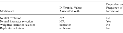
In the classical evolutionary selection model, variant replicators differ in fitness, a value associated with each replicator, and differences in fitness result in differential replication. We will call this classical selection model replicator selection: there is a value directly associated with the replicator that leads to its differential replication.

In language change, replicator selection models the classical sociohistorical linguistic theory. In this theory, different variants have different social values associated with them. By virtue of the social values associated with the variable, some variants are propagated at the expense of other variants. In the earlier versions of the model, factors such as social class, education level, and gender are correlated with linguistic variants. However, these correlations are interpreted as representing other, less easily measured factors, for example, that a higher social class is perceived as more prestigious than a lower social class, and so the actual social value associated with the variant is a higher degree of prestige (e.g., Labov, Reference Labov1972:290). More recently, it has been hypothesized that the social value associated with a linguistic variant that speakers use in choosing that variant is the group identity associated with that variant (LePage & Tabouret-Keller, Reference LePage and Tabouret-Keller1985:181–182). This is the theory that Trudgill rejected for new-dialect formation in an isolated speech community.

However, change by replication can happen without (replicator) selection operating. Because there is a degree of randomness in the replication process, there will be random fluctuations in replicator frequencies as reproduction takes place in a finite population. If the fluctuation happens to hit zero, then the replicator goes extinct. Thus, change takes place in the population simply by virtue of random processes; no selection has taken place. This process is called genetic drift (Crow & Kimura, Reference Crow and Kimura1970); genetic drift is very different from linguistic drift. The process is also called neutral evolution, and we will use this term to avoid confusion.

In language change, a neutral evolution model corresponds to Trudgill's deterministic model. A significant property of neutral evolution models is that the probability of fixation—fully successful propagation of a variant—is a function of the frequency of the variant. Neutral evolution is a probabilistic model, which is fundamentally different from a model that predicts that the majority variant will always win out. However, because Trudgill's theory is invoking the same usage-based processes as we are, namely that speakers alter their behavior in response to the language they hear around them, and those usage-based processes are probabilistic, then it is not implausible to consider Trudgill's theory in probabilistic terms, as we will do. Trudgill himself predicted that speakers “simply selected, in most cases, the variants which were most common” (Trudgill, Reference Trudgill2004:115, emphasis added).

Neutral evolution models include processes that lead to differential replication. This can best be understood by considering the closest biological parallel, which is a group of islands in which each contain a set of individuals of different species or alternatively individuals who have a particular gene that has different variants. Here speakers are equivalent to islands and utterances to migrations of individuals between islands (Blythe & McKane, Reference Blythe and McKane2007). Even though no species or allele is favored over another, if one island is geographically closer to another, for instance, then the chances of interaction between these islands are greater. More generally, the nature of the network of islands and the strengths of the interactions between the islands would appear to have an influence on the evolutionary process. In the GAS, as defined earlier, this process is a type of selection: interaction of an interactor with its environment causes replication to be differential. What is unusual is that the environment in this case is another interactor. We will call this process interactor selection, to differentiate it from classical replicator selection.

In language change, structured social networks mean that a speaker is more likely to interact with certain speakers rather than others. In this sense, social distance replaces the geographical distance used in the biological example (though geographical distance contributes to social distance). Because the interaction results in the replication of some linguistic variants (replicators) over others in language use, depending on the language produced by the speakers one interacts with, it can bring about differential replication. We will call this type of interactor selection neutral interactor selection, in that the only factor that influences replication is the frequency of interaction with the interactor.

Trudgill allowed for neutral interactor selection in his deterministic theory. Neutral interactor selection is essentially accommodation to the speech of one's interlocutors. Earlier, we noted that Trudgill proposed that women are more advanced in the use of New Zealand English variants because female children interact more with older women than with older men. This is neutral interactor selection: women speak more to women than to men. Neutral interactor selection is a possible mechanism for another effect observed in the Stage II ONZE project speakers. The use of variants is partly correlated with the ethnicity of the speaker's parents (Gordon et al., Reference Gordon, Campbell, Hay, Maclagan, Sudbury and Trudgill2004:263; see also Trudgill's example of Mrs. German). Presumably this is because children speak more to their parents (at least at first) than to other members of the community. This was particularly likely before schooling became common (the New Zealand Education Act mandating compulsory primary education was passed only in 1877).

There is another type of interactor selection that is possible in language change. In this type of interactor selection, interactors (interlocutors) are preferred or dispreferred by a speaker no matter how frequently or infrequently she interacts with them, and their linguistic replications (utterances) are weighted accordingly. Thus, variants of a speaker whose productions are weighted more heavily will be differentially replicated. This type of interactor selection is unlike network structure, in which the weighting of variants is simply a consequence of frequency of interaction with different speakers producing different variants. We will call this weighted interactor selection, because interactors are weighting the productions (replicator replications) of particular interactors differently; no matter what the frequency of interaction with them is.

Weighted interactor selection implies that a speaker's linguistic behavior is influenced not just by frequency of interaction but also a differential social valuation of particular speakers, possibly because of the social group to which they belong. It is not clear whether Trudgill would have considered weighted interactor selection to conform to his model. However, Trudgill described his theory as deterministic and made assertions such as “the minority quite simply and mechanistically accommodated to the majority” (Trudgill, Reference Trudgill2004:148) and “the new colonial dialects are a statistical composite of the dialect mixture” (ibid., 123, emphasis original). These statements imply that Trudgill did not allow weighted interactor selection in his deterministic theory.

The four mechanisms are summarized in Table 4.

Table 4.

Mechanisms for propagation of variants

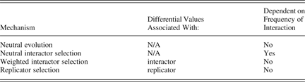
Because Trudgill's theory excludes replicator selection and (apparently) weighted interactor selection, in order to test Trudgill's deterministic theory of new dialect formation, we need only investigate models of neutral evolution and of neutral interactor selection. Our aim is to push models of neutral evolution and neutral interactor selection as far as possible to see if they can model the emergence of a new dialect without having to resort to replicator selection or even weighted interactor selection.

THE DESCRIPTION OF THE MODEL

The model we have constructed was first described in Baxter et al. (Reference Baxter, Blythe, Croft and McKane2006, section III). Here we summarize it in a slightly more qualitative way and refer the reader to Baxter et al. (Reference Baxter, Blythe, Croft and McKane2006) for a more mathematical treatment.

Trudgill's theory does not imply any interaction between sociolinguistic variables (linguemes), and we similarly assume that they are independent.Footnote ³ This allows us to focus on a single lingueme, which we assume can exist in several variants denoted by α, β, γ, … . The speech community consists of N speakers, labeled by an integer i that runs from 1 up to N. Each speaker will have a grammar—knowledge about their language—that includes her perceived frequency of the variants of the linguemes/sociolinguistic variables, in conformity with the principles of the usage-based model of linguistic representation. For example, the frequency of H-retention—the variant with the phoneme /h/ in particular contexts—in the English of early New Zealand was 75%, and the frequency of H-deletion is therefore 25% (Trudgill, Reference Trudgill2004:116). If this fact represents what speakers are exposed to, then their knowledge about New Zealand English at the time includes this frequency information.

Because we are focusing on one lingueme, the grammar at a particular time, t, can be considered to be the set of perceived frequencies of the variants of that one lingueme at this time. To formulate this mathematically, we assume, to make the description of the model easier, that there are only two variants, α and β. Then the grammar of speaker i at time t can be specified by x _i(t), where x is the perceived fraction of time the α variant is used, and (1 − x) is the perceived fraction of time that the β variant is used. For example, the grammar of speaker 3 could at some time be such that x ₃ = .9. This would mean that, because 1 − x ₃ = .1, she would perceive that the α variant is nine times more likely to be used than the β variant. The state of the language at time t is the set of the grammars of the individual speakers: {x ₁(t), x ₂(t) …, x _N(t)}.

The aim of the model is to see how the fractions x _i change with time due to the various interactions between the speakers. The first thing that has to be done is to set the initial values of these fractions. These could be taken to be random numbers between 0 and 1, or they could have a more specific form. For example, all speakers could have x = .5 initially, so that the α and β variants are perceived to be equally likely by all speakers. After choosing this initial condition, we allow the grammar of the population of speakers to evolve with time. We do this by repeating three steps in sequence: social interaction, reproduction, retention.

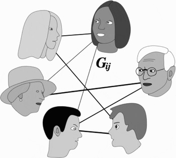
In the first step, social interaction, a pair i,j of speakers is chosen to interact (hold a conversation). Some speakers could in principle be favored over others, simply because they are very well connected. Conversely, isolated speakers might have less chance of being picked. To model this, we give a probability for each pair of speakers to be picked and make the choice on the basis of this. This probability is denoted by G _ij. G _ij represents simply the likelihood of occurrence of a linguistic interaction between two speakers; it is symmetric because if speaker i interacts with speaker j, then speaker j necessarily interacts with speaker i. G _ij reflects the geographical and social structure of the network of speakers; it models neutral interactor selection. This is illustrated in Figure 1.

Figure 1.

Speakers in the society interact with different frequencies (shown here schematically by different thicknesses of lines connecting them). The pair of speakers i,j is chosen to interact with probability G _ij.

So, in practice, a pair i,j of speakers are selected with a prescribed probability G _ij.

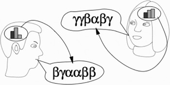
In the second step, reproduction, each of the speakers selected in step 1 are now allowed to interact by first one of the individuals producing 10 or 20 (in general, T) tokens of the lingueme, and then the other doing the same. For example if T equals 10, 8 of these might be in the α form and 2 in the β form. To reflect the stochastic nature of the communicative process seen in real conversations (that is, that all language behavior is variable and probabilistic), the number of α or β variants will reflect the state of the grammar of the speaker, but will be random in the same way that a coin toss or the roll of a die is random. To take a simple example, suppose for speaker i that x _i = 5/6, then we can roll a die to see whether an α or β variant should be uttered; if a 1 was rolled, the β variant would be uttered, but if any other number was rolled, the α variant would be uttered. If T = 12, for instance, then it would be most likely that 2 β and 10 α variants would be uttered. But this would only be the most likely scenario. It could be that 9 or 11 α variants were uttered, or even 12, with no β variants being uttered at all. It is the stochastic nature of these events that ultimately leads to particular variants becoming extinct from the population. When only one variant is left, we adopt the language of population genetics and say that it has become fixed. In general we can imagine tossing a (biased) coin—with a probability x _i of coming up heads—T times to see how many α variants are produced by speaker i in a particular utterance.

After speaker i has produced an utterance, speaker j produces a sequence of tokens according to the same prescription, but using their grammar. This is illustrated in Figure 2.

Figure 2.

Both speakers i and j produce an utterance, with particular lingueme variants appearing with a frequency given by the value stored in the utterer's grammar. In this particular case three variants are shown (α, β, and γ) and the number of tokens, T, is equal to 6.

We now need to describe the effect of these utterances on the listener—and also on the speaker who made the utterance.

The final step, retention, is to modify each speaker's grammar to reflect the actual language used in the course of the interaction. The simplest approach is to add to the existing speaker's grammar additional contributions that reflect both the tokens produced by herself and by her interlocutor. The weight given to these tokens, relative to the existing grammar, is given by a parameter λ. This parameter can be thought of as the receptiveness of the speaker to changing her grammar on the basis of the language she hears. Presumably, there will be a large amount of inertia in the retention of a grammar, and therefore λ will be small. The utterance that has just been produced will only have a small effect on the existing grammar. It is the cumulative effect of utterances over many interactions that will lead to a significant change in the grammars of the speakers.

The weighting of existing tokens relative to new tokens represented by λ brings about a reduction in the weight of existing tokens that continues every time new tokens are added to a speaker's memory. This reduction of weighting of older tokens is equivalent to their decay in memory. The rate of decay is controlled by λ, and if λ is small, as just described, the decay function is close to the exponential form widely used in psychological models of memory (see Anderson & Schooler, Reference Anderson and Schooler1991:396). After a token's memory has decayed to a value ε, the token is defined to be forgotten. The forgetting of tokens is what allows propagation/extinction to take place. After all tokens of one variant are forgotten, that variant is no longer produced and has gone extinct.

Conversely, retention in memory of a particular variant is dependent on continuously hearing new tokens of the variant. Our model of entrenchment in memory is broadly compatible with three general results. The first is that exposure to tokens distributed over time rather than massed at once facilitates entrenchment or consolidation of the memory (see Rovee-Collier, Reference Rovee-Collier1995:148, and references cited therein). In our model, the value of x _i is higher if the corresponding tokens arrive uniformly over some time interval than if they were committed to the store at the start of it.

The second result is that there is a lower limit to the rate of decay imposed by consolidation of memory. This has been discussed in terms of a time window for laying down a memory (Rovee-Collier, Reference Rovee-Collier1995). If time between two tokens of the same variant is longer than the time window, then the new tokens do not help to consolidate the memory trace of the original tokens, and the memory is not entrenched (i.e., the older memory traces decay [Rovee-Collier, 1995]). In our model, we can define a time window through the length of time it takes for the memory of a token to decay to the level ε that arises for a particular choice of the parameter λ. As we will discuss in detail, the fact that the time window has been reported to be about two days in infants (Rovee-Collier, Reference Rovee-Collier1995), and somewhat longer in adults, imposes a minimum decay rate λ.

The third result is a linguistic generalization. Linguistic forms with a higher token frequency are more likely to be retained, whereas linguistic forms with a lower token frequency are more likely to be replaced with novel variants (see, for example, Bybee [Reference Bybee1985] on the replacement of low token frequency forms in a morphological paradigm, Bybee and Slobin [Reference Bybee and Slobin1982] and Lieberman, Michel, Jackson, Tang, and Nowak [Reference Lieberman, Michel, Jackson, Tang and Nowak2007] on the replacement of irregular forms in low token frequency words, and Phillips [Reference Phillips1984] on the replacement of the “underlying forms” of low token frequency variants). This linguistic generalization follows from the first two results about memory. The lower the token frequency, the greater the memory of each one decays between the arrival of individual instances, thereby making it less likely new tokens will contribute to the entrenchment of the variant.

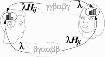
The weight, relative to her own utterances, that speaker i gives to speaker j's utterances is specified by a number H _ij. This is intended to reflect the interlocutor's social status and other social effects, and models weighted interactor selection. H _ij is asymmetric: speaker i may not give the same weight to speaker j's utterance that speaker j gives to speaker i's utterance. For the purpose of testing Trudgill's theory, we begin by taking H _ij to be the same for all pairs i and j, denoted by the constant H (i.e., H _ij is symmetric and the same for all speakers), to see if the data can be explained without having to resort to social effects of this kind.

To specify how exactly x _i changes during this time step, let us denote x _i at time t by x _i(t), as before, and x _i at time t + 1 by x _i(t + 1). Also suppose our random number generator (the die or coin described earlier), produces n α variants for speaker i and m α variants for speaker j. Then x _i(t) will be modified by two factors: (i) we will have to add a factor of λn/T to x _i(t), because n/T is the fraction of α variants given in speaker i's utterance and λ is the weight we are giving to them; (ii) we will also have to add a factor of λH _ijm/T to x _i(t), because m/T is the fraction of α variants given in speaker j's utterance, λ is the weight we are giving to them, and H _ij is the relative weight that speaker i gives to speaker j's utterances. In terms of equations

There will be a similar rule for speaker j, but with i and j interchanged and the numbers n and m interchanged. Figure 3 illustrates this step.

Figure 3.

After the utterances have been produced, both speakers modify their grammars by adding to them the frequencies with which the variants were reproduced in the conversation. Note each speaker retains both her own utterances as well as those of her interlocutor, albeit with different weights.

We have used the symbol ∝ \, \propto \,(proportional to) in this equation, rather than an equality symbol. To see why this is, we imagine that we start from the fraction of the β variant in the grammar and carry out the same exercise. This would increase also, due to the addition of terms. So the fraction of α and β variants at time t + 1 when added together would be greater than 1. To remedy this, we have to divide the right-hand side of the equation by a factor of 1 + λ+ λH _ij, which guarantees that the sum of the fraction of α and β variants add up to 1 at all times. Dividing by this factor means that we can replace the proportionality symbol by an equality symbol.

Having carried out these three steps, we now pick another pair of speakers at random and continue in this way for a large number of time steps until the x values have been modified significantly. In the absence of other factors, the final state will be when either the α or the β variant dies out completely: all the x _i are either 0 or 1. One of the questions of interest is: How long on average is it before this fixation happens? This may be investigated both mathematically and using computer simulations. To carry out the latter, a particular network structure has to be assumed. In the next section, we will see that it can be shown mathematically that in many cases the time to fixation is independent of the network structure. However, here we briefly consider two examples of speaker networks that we might expect to be applicable to the early colonial period in New Zealand.

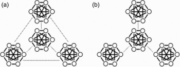
The first is the “equal-groups” network, which might model several isolated homesteads in occasional contact with each other. The simplest case would consist of l groups of M speakers, so that N = Ml. Speakers within a particular group would all be interconnected and interact with the same strength, but there would only be weak interaction between the groups, perhaps mediated by a single speaker from each group. This is illustrated in Figure 4a. As townships formed, this network structure might be replaced by a “hub-and-spoke” network, which is as in the equal-group case, but with one group (the hub) being bigger than the others (not indicated in the figure), and with the other (l − 1) groups interacting with each other via the hub. This is shown in Figure 4b.

Figure 4.

Illustration of two network structures. (a) A community divided into a number of equal groups within which interactions are frequent but between which are less so: the dotted lines are intended to indicate interactions between one or more pairs of speakers from different groups. (b) A “hub-and-spoke” community in which there is one central (hub) group and several peripheral (spoke) groups. No interactions take place between different spoke groups, but all spokes interact with the hub.

These two network models imply that there are strong network ties among the speakers within the groups but weak ties between speakers of different groups (cf. Milroy, Reference Milroy1987).Footnote ⁴ Trudgill however also suggested that early New Zealand society as a whole was made up of weak ties, as we already noted. Such a society would be better modeled by a relatively “flat” network in which all speakers have equal likelihood of interacting with all other speakers.

Clearly many other network topologies may be postulated. Fortunately, as already mentioned, we will not need to specify the topology to find the mean time to fixation (see also the Mathematical Appendix in the online version for discussion of different network structures). Both this result and more details of our investigations of the model are discussed in the next section.

PROPAGATION BY NEUTRAL INTERACTOR SELECTION

In this section our aim is to explore whether the mathematical model described in the previous section reproduces behavior actually observed in the emergence of New Zealand English with empirically plausible parameter settings. Specifically, we wish to determine whether the main features of the empirical data—namely, that variants initially in the majority were in almost all cases adopted by all New Zealand English speakers in the space of about 50 years (Trudgill, Reference Trudgill2004:23)—can be explained by neutral interactor selection alone, as Trudgill proposed.

We focus initially on an idealization in which the community of speakers has a fixed size over the relevant historical period. This is a simplification of the true situation, in which old speakers die and new speakers are born or continue to arrive through immigration. However, this simple case is still useful to us in evaluating Trudgill's deterministic theory because we can obtain quite general mathematical results and then see (e.g., by means of computer simulation) how these are affected as progressively more realistic features are introduced into the model. These extensions will be described in the next section.

As described in the previous section, the model is stochastic: every time it is run, a different outcome might be realized. To make comparisons with the empirical data, we must therefore determine how likely a particular outcome is to be obtained within the model, or how such an outcome is typically reached.

In particular, we noted that if initially a lingueme has multiple variants, eventually all but one of them will go extinct in the model. The probability that a specific variant, say α, fixes (i.e., is the only one remaining after a large number of interactions) can be calculated exactly. We focus specifically on the case of neutral interactor selection, in which all speakers ascribe the same weight to others' utterances: mathematically, this means setting all H _ij parameters to the same value. Then, the model predicts that variant α fixes with a probability equal to its initial frequency across all speakers' grammars. For example, if some fraction x of speakers all initially use only variant α, and the remaining fraction initially do not use α at all, the probability that α fixes is x. The same fixation probability is also obtained if all speakers initially use α a fraction x of the time in their speech. This result (whose derivation is given in the online Mathematical Appendix) holds no matter how large the community of speakers is, what its network structure is, how large the common value of H _ij is, or how the variants are initially distributed among speakers as long as the only type of selection operating is neutral interactor selection. Therefore, it is not necessary for us to know any of these parameters in order to predict fixation probabilities from the model within the constraints imposed by neutral interactor selection.

The most likely outcome of the model is that all the variants that are initially in the majority go to fixation. If there are variants that are initially in a slight minority, their chances of fixation are almost as high as that of the majority variants. This provides support for Trudgill's majority rule, and, in particular, the observation that the relevant initial frequency is not the number of speakers using a particular variant, but the token frequency (Gordon et al., Reference Gordon, Campbell, Hay, Maclagan, Sudbury and Trudgill2004:239–241). In our model, the grammar frequency corresponds to the frequency with which a speaker produces tokens of a particular variant. Furthermore, the stochastic nature of the interactions allows minority variants to fix without the need to invoke special mechanisms such as (linguistic) drift (Trudgill Reference Trudgill2004:129–47). Two minority forms that did fix in the formation of the modern New Zealand English variety were the weak vowel schwa, initially used by 32% of the Stage II ONZE speakers (Trudgill, Reference Trudgill2004:119) and fronted and lowered strut vowels, initially used by 34% of the Stage II ONZE speakers (Trudgill, Reference Trudgill2004:136; see earlier discussion). Unfortunately it is not clear what fraction of tokens these speaker percentages correspond to. Under the assumption that speakers were initially using these variants consistently (i.e., only ever-produced tokens of a single variant), the token frequencies and speaker frequencies would coincide. Then, the model predicts that fixation of both minority forms through purely random effects would occur with probability .32 × .34 = .1088, about 11%. That is, there is an 11% likelihood that under a neutral evolution model, minority variants with 32% and 34% occurrence will go to fixation. This is a sufficiently high likelihood that the minority variants went to fixation simply by chance. Therefore the hypothesis that propagation of these variants was due to some process other than neutral interactor selection alone, such as markedness or linguistic drift, cannot be accepted with a high degree of confidence.

We now turn to possibly the most striking aspect of the ONZE data: that a relatively uniform New Zealand English dialect was established in a community of between 100,000 and 600,000 speakers in the course of 50 years (see Table 1, 1861–1890). Trudgill (Reference Trudgill2004:113) wrote,

As noted previously, Trudgill indicated that this stage takes approximately 50 years, or two generations, to emerge (Trudgill, Reference Trudgill2004:23), although Trudgill did acknowledge that some of the ONZE project speakers born after 1890 did not have a recognizably New Zealand English dialect (Trudgill, Reference Trudgill2004:24).

Again, each run of the model yields a different time to fixation of a single variant. We therefore ask what the mean time to fixation is over many different runs, averaged over those runs in which the variant of interest actually became fixed. It is this value that we will compare with empirical data. An anonymous reviewer pointed out that language changes rarely go to complete fixation. However, the mean time to near-fixation will be on the same time scale as the mean time to complete fixation.

Analysis of the model, outlined in the online Mathematical Appendix, leads to the result that for the vast majority of network structures, the number of interactions that need to take place on average until fixation occurs is independent of the network structure. Intuitively, one might expect a variant used by a speaker who interacts frequently to be more likely to fix, or fix more quickly, than one used by an infrequently interacting speaker. However, fixation is a property of the whole system, not just a particular individual; so the infrequently interacting speaker still has to have used or heard the variant enough times to reach the state of fixation. Changing the structure of the network does not affect this time in those cases where the time it takes for the initial awareness of the variant to spread across the network is much less than the fixation time. These are in fact the vast majority of cases (see the online Mathematical Appendix). Some extreme cases (such as chains of speakers or very narrow bottlenecks between different groups) would in fact increase the fixation time (see the discussion of Equation (2)).

This number of interactions is given by the following combination of model parameters:

(1)

In this equation, N is the number of speakers; T is the number of tokens exchanged per interaction; λ is the parameter controlling the rate at which speakers' grammars are allowed to change; x is the variant's initial frequency; and all interaction parameters are set to a common value H _ij = λh. (The appearance of λ here is due to technical reasons discussed in Baxter et al. [2006]).

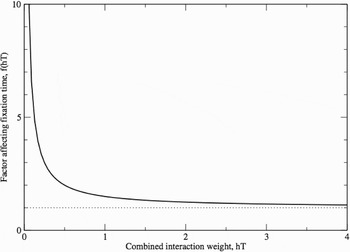
The notation f(hT) indicates the presence of a factor contributing to I _fix through the product of the interaction parameter h and the number of tokens uttered per interaction T. This factor is plotted as a function of hT in Figure 5 and can be seen to be slowly varying and close to 1 when this product is large, but diverging rapidly if it is small.

Figure 5.

The factor f(hT) appearing in Equation (1) for the number of interactions until fixation, plotted as a function of the combined interaction weight, hT, which is the product of the interaction weight h given to a single utterance from another speaker and the number of tokens per utterance T. As hT gets ever larger, the factor approaches the value 1 (the dotted line) from above.

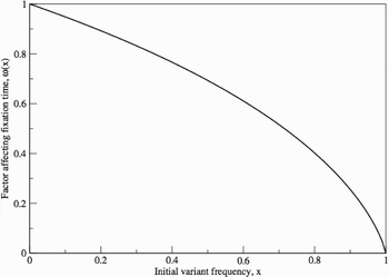
In practice, the latter occurs only if h is very small, because T is by definition at least 1. This reflects the fact that the number of interactions needed until fixation occurs is very large if speakers give only a very small weight to others' utterances. Similarly, the initial variant frequency x contributes another factor ω(x) to I _fix, which we have plotted in Figure 6.

Figure 6.

The factor ω(x) appearing in Equation (1) for the number of interactions until fixation, plotted as a function of the initial frequency x of the ultimately surviving variant.

The shape of the curve indicates that variants with an initially high frequency tend to fix more quickly in the model than those with a low initial frequency, as one might expect. The mathematical forms of both factors are presented in the online Mathematical Appendix for the interested reader.

To make a comparison of Equation (1) with empirical data, there are two specific problems to overcome. First, we need to find a way to convert the number of interactions to a real time; and second we need to relate the abstract model parameters λ and h to real-world quantities. (We regard N, T, and x as, at least in principle, measurable quantities).

The first task is achieved by estimating how many tokens of a linguistic variable a single speaker is likely to be exposed to in her lifetime. We call this number T* (the asterisk distinguishing it from the number uttered per interaction). Then, because T tokens are uttered per interaction, the number of interactions per speaker lifetime is given by T*/T.

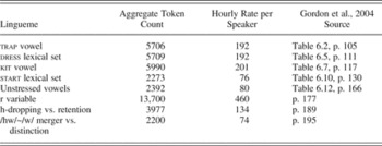
Of course, one expects a huge variation in T* over all possible variables. We focus therefore specifically on those analyzed in the ONZE project, which were mostly vowel variables and a few other phonetic features. In Gordon et al. (Reference Gordon, Campbell, Hay, Maclagan, Sudbury and Trudgill2004), token counts were presented for eight linguemes aggregated over interviews with 59 speakers of Early New Zealand English. These data are summarized in Table 5.

Table 5.

Rate of occurence for eight different linguemes analyzed quantitatively in one ONZE data

In order to estimate T*, we need to convert these token counts into rates per speaker, which in turn demands knowledge of the length of the interviews conducted. This information is not presented in Gordon et al. (Reference Gordon, Campbell, Hay, Maclagan, Sudbury and Trudgill2004), but can be estimated by identifying the relevant recordings in the catalog held by the New Zealand Radio Sound Archives.Footnote ⁵ We found the recordings of 55 of the 59 speakers listed in Gordon et al. (Reference Gordon, Campbell, Hay, Maclagan, Sudbury and Trudgill2004:334–37). Taking into account that some recordings involved multiple speakers (by dividing the time of the recording equally between them), we found the mean recording length over these 55 speakers to be 30 hr 15 min. From this we can deduce the hourly per-speaker token rate also presented in Table 5. We have since been informed (Jennifer Hay, personal communication) that, in fact, only a subset of the tokens uttered by each speaker were included in the token counts given. Therefore, the actual token rate would be higher than that given in Table 4, at least in the type of speech produced in an interview situation. As it happens, the mathematical analysis we are about to describe calls for us to use the smallest reasonable value for T* so that neutral interactor selection has the greatest chance of explaining the empirical data. Thus we will take the smallest rate from Table 4, assume that on a typical day a speaker produces at least as much speech as they would in a 1-hour interview, and further assume a 50-year lifespan for each speaker (as data for life expectancy in the late nineteenth century suggestFootnote ⁶). This leads to a lifetime T* estimate of approximately 1.3 million tokens (although one should bear in mind that the true value is likely to be much higher).

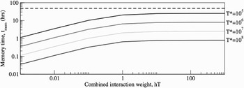
With the connection between the number of interactions and a real time fixed by T*, our strategy now is to vary the unknown parameter λ so that the mean time to fixation given by Equation (1) corresponds with the observed 50 years. It then remains to decide if this value of λ is empirically plausible. Recall that λ controls the amount to which tokens uttered in the previous interaction affect the grammar. We can ask how many interactions are needed until the intensity of a stored token in the memory drops to some fraction ε of its initial value. For example, if ε = 0.01, this would correspond to time taken for the initial intensity to decay to 1% of its original value. We call this time the memory time, and, as a fraction of a speaker's lifetime, will denote it t _mem. In the online Mathematical Appendix, we show that for fixation to occur in 50 years, t _mem for at least one speaker in the community must satisfy the relationship

(2)

Again, this relationship holds for any social network structure comprising N speakers, as long as propagation is by neutral interactor selection alone. There are two reasons why this expression is written as an inequality rather than as an equality. First, there are a small number of networks for which I _fix exceeds the value given by Equation (1). Second, the memory lifetime imposed by a particular value of λ varies from speaker to speaker in models in which different speakers interact with one another with different frequencies.

The inverse relationship between the upper bound on the memory window t _mem and the token frequency T* is at first sight puzzling. Intuitively, it seems that the more frequently a new variant is used, the faster it would reach fixation. However, the old variant is used frequently too. For fixation to occur, the collective memory of the old variant must be erased, and this can only be achieved if individual speakers are prepared to forget single utterances on a short timescale. In short, the elimination of the old variant is the crucial limiting factor for the fixation of the new variant. The variants of a phonological variable such as H-retention are variant pronunciations of particular words (i.e., those with an etymological h). Although those words may occur at a rate high enough for the word as whole to be retained in memory, one variant of a phoneme in the word such as (h) may decline in use to too low a rate for a speaker to retain that phoneme variant in memory. If the speakers collectively are no longer exposed to this variant at a rate sufficient to retain it in memory, then it is lost, and the other variant then achieves fixation (in the case of a variable with two variants).

The question then arises: What is an acceptable range for the rate at which an individual token is forgotten, that is, t _mem? This is the time window within which exposures must reoccur for this consolidation to take place (Rovee-Collier, Reference Rovee-Collier1995; see earlier discussion). For infants (aged 3 to 6 months), this time window is about 2 to 4 days for a range of learning tasks; for adults, these windows appear to be longer, in fact, much longer (Rovee-Collier, Reference Rovee-Collier1995). Therefore, if a speaker's t _mem is required to be less than 2 days for community-wide fixation to occur in 50 years, we have a criterion for rejecting the model of propagation by neutral interactor selection.

So that this rejection criterion is invoked with the smallest likelihood, we choose parameter values that make the right-hand side of Equation (2) as large as is reasonably consistent with the empirical data. That is, we choose the smallest N and T* suggested by the data. From Table 1, we see that the smallest N during the period of interest (1864 to 1890) is about 100,000. We have argued for an underestimate on T* of 1.3 × 10⁶. Because ω (x) is a decreasing function of x, we should also focus on the lingueme variants reported by Trudgill (Reference Trudgill2004) to have been in a healthy majority among the Stage II ONZE speakers. Two features, H-retention (Trudgill, Reference Trudgill2004:116) and diphthong shift (ibid., 121), were reported as being initially used by 75% of speakers, so we shall take x = .75 as a representative value.

In Figure 7, we plot the memory time appearing on the right-hand side of Equation (2) as a function of the product hT for various T*, N = 100,000, x = .75 and ε = .01. This means that every possible combination of the unknown parameters T and h is included somewhere on the graph. Note that the data have been plotted on logarithmic axes, which means that even with the smallest T* plotted—10⁵, which is an order of magnitude lower than our earlier underestimate—memory times imposed by the model are already an order of magnitude shorter than the minimum 2-day time window, and even smaller for larger (and probably more realistic) values for T*.

Figure 7.

The memory time appearing on the right-hand side of Equation (2) that is imposed on the model by requiring fixation to occur within 50 years, as a function of the (unknown) combined interaction weight hT appearing in Figure 4 (T is the number of tokens exchanged in an interaction, and h is the fixed weighting of tokens). As described in the text, we have taken N = 100,000, x = .75, and ε = .01 for values of T* ranging from 10⁵ (top curve) to 10⁸ (bottom curve). For the linguemes relevant to the ONZE project, the data suggest that T* of at least 10⁶ is appropriate. The dashed line is the shortest memory time that we deem plausible (see text). Note that both axes are logarithmic: although the longest time window (largest h, smallest T*) is only half that of a human infant, the shortest (smallest h, largest T*) is 1000 times shorter.

Bearing in mind that Equation (2) is an overestimate of a speaker's memory time, and that we have deliberately erred on the side of caution with the values of N, T*, and x, we believe Figure 7 provides compelling evidence that neutral interactor selection is unlikely to be solely responsible for the fast convergence of the New Zealand dialect to a homogeneous, stable variety. Although this conclusion is based on our having set the forgetting parameter ε to the somewhat arbitrary value of .01 (1%), we note that for the case T* = 10⁶ suggested by the data, the curve in Figure 7 can be made to approach the desired two-day memory window for large hT only if ε is reduced to approximately 10⁻¹², an unfeasibly small number. So although we are confident that our argument is correct, this aspect would benefit from further study. This is discussed once more in the final section, but for the moment, we note that not only would larger, and more empirically reasonable, values of N and T* demand an even smaller value for ε, but also that extensions to the model that include more realistic features also have the effect of extending fixation times, and hence further reduce the t _mem that is imposed. These effects are the subject of the next section.

MODELING GENERATIONAL REPLACEMENT

In this section, we add generational effects to our model of neutral interactor selection. The effect of the presence of speakers born at different times is an integral part of Trudgill's account. His three stages correspond to three generations: immigrants, first-generation native New Zealanders and second-generation New Zealanders. Trudgill uses the simplifying assumption that each generation is discrete and separate in time (Trudgill, Reference Trudgill2004:24). This is a stylized representation of demographic reality, but we will begin by modeling these three distinct generations. In this section, we will show that this generational model—and even more realistic models of speakers of differing ages—does not ameliorate the difficulty that fixation cannot occur within 50 years and in fact makes the situation worse.

In the previous section, we used the most optimistic condition that all speakers had the same receptiveness to language use around them as children. Now we assume that children are more adaptable in their language use than adults are— that is, adults are less adaptable than children. It seems clear that if some of the speakers in the population change more slowly than in the model in the previous section, the time taken for the population as a whole to reach fixation must be longer. This is borne out in simulations, which we now describe.

To represent the difference in susceptibilities between children and adults, in our first simulation speakers are assigned a constant value of the update parameter λ for the first half of their lifetime, which represents childhood. In the second half of their lives, the adult stage, speakers interact as normal, but their grammars are not updated at all, that is, λ is set to 0 for these speakers. The generations overlap, so that each generation's child phase coincides with the previous generation's adult phase, as represented in Figure 8.

Figure 8.

Schematic representation of the three discrete generations. The immigrant generation arrives as adult speakers. Each subsequent generation begins as children then changes into adults. At the same time, the adults are removed. The colored traces represent the overall proportion with which each generation uses the first variant (α).

At any time, two generations coexist, one in an adult stage and one in a child stage. We make the further simplification that the original generation of immigrants is already in the adult phase at the beginning of the simulation, and they speak with a fixed grammar representing their original dialects (this assumption has been questioned empirically and will be relaxed in the following discussion). All other aspects of the model described previously remain unchanged.

In this model, the rudimentary leveling and other changes in Trudgill's first stage (Trudgill Reference Trudgill2004:89–99) are considered to be sufficiently minor that we can neglect them for our current purposes. The probability that a variant reaches fixation in our model is dependent only on its initial proportion and not on the number or value of the other variants (Baxter, Blythe, & McKane, Reference Baxter, Blythe and McKane2007). Because we are interested mainly in the fate of the major variant that eventually fixes, it is sufficient for our current purposes to consider a model with only two variants—it makes no difference in the model whether the second variant represents a single variant or the collective frequency of all the minority variants. The early elimination of small minority variants makes no difference to the probability or eventual time to fixation of the majority variant, provided the initial frequency of this variant is set correctly. Similarly, small amounts of accommodation by adult speakers in the first stage would not significantly alter the frequencies with which the (main) variants are used in the population as a whole, and therefore, this has only negligible impact on the mean time to reach fixation.

In repeated simulations of this model, we found that the children as a group duplicated the overall proportion of variants used by the adults, but individually there was a large variation between speakers. This can be seen in Figure 9 in which the proportion of speakers who used variant α with a frequency x lying in a narrow range is represented by a vertical bar covering that range.

Figure 9.

The distribution of speaker's grammar values x (the frequency with which variant α is used) in each of the three generations. The immigrant generation is fixed at the initial conditions (in this case, 40% use exclusively variant α and 60% variant β) whereas subsequent generations conform to a distribution resulting from the interaction dynamics. Results shown are for a population of 60 speakers with interaction parameter h = .2 and child susceptibility λ = .05. Distributions have been averaged over 100 repeats of the experiment.

The bars just below 0 and just above 1 represent the proportion of speakers that use exclusively variant β or exclusively variant α, respectively, at the end of each generation. Forty percent of the immigrant generation used exclusively variant α, whereas the remainder used exclusively variant β. The results shown in the figure are for a relatively small population, but the shape of the distribution shown depends only on the interaction parameter h and not on the population size (it is very similar to the quasistationary distribution described in Baxter et al. [2006]). Several different values of T*, the number of tokens each speaker hears in a lifetime, were tried, but it was found that an equilibrium distribution was reached relatively quickly in each generation and did not change when generations ran for a larger number of interactions.

In the first generation, all speakers used both variants (the proportion of speakers who use exclusively one variant is zero), but most speakers used one variant a large majority of the time: some speakers used mostly variant β, and others used mostly variant α. This distribution arises because the children's grammars drift due to the stochastic nature of the model and their interactions with each other, with the feedback from a speaker's own utterances tending to drive her grammar toward a majority of one variant. On the other hand, because the children continue to hear examples of both variants from the immigrant generation adults (and in the original proportions), the overall proportion of variants used by the first generation tends to stay fairly close to that used by the immigrant generation. This situation is qualitatively similar to the intra- and interindividual variability of Trudgill's Stage II (Trudgill, Reference Trudgill2004:101–108). Individual speakers differ from one another, their usage can be variable, and the overall mixture reflects the range and frequency of variants available. It should also be noted that this variation appears in the early stages of any model in which speakers can drift, even if there is no inclusion of different generations of speakers.

More problematic for Trudgill's thesis is that the second generation repeats this process in relation to the first generation, learning a similar overall frequency of variant use and settling on a very similar distribution of frequencies of use among different speakers, as can be seen in the rightmost panel of Figure 9. In Figure 8, the overall proportion of variant α used by each generation is represented by a colored trace. We see that each generation shows some variation during their childhood phase, but the frequency does not move very far from that used by the previous generation in their adult phase. This pattern continues over subsequent generations, with a small random variation between generations until one variant finally becomes fixed. The amount of change from one generation to the next is independent of the number of tokens each speaker hears in her lifetime (T*) and is instead governed by the size of the population and the strength of the interaction between speakers (the parameter h of the previous section). The effect of the presence of a “frozen” adult generation is to inhibit fixation. The time taken to reach fixation for a population of 100,000 speakers and small values of h is typically hundreds of generations. The number of generations required to reach fixation actually increases with larger values of h.

We also investigated allowing adult speakers to modify their grammars a little. There is evidence that adult speakers are able to vary their usage of linguistic variants to some degree (Harrington, Palethorpe, & Watson, Reference Harrington, Palethorpe and Watson2000; Sankoff & Blondeau, Reference Sankoff and Blondeau2007), so a model allowing this possibility is empirically more plausible. The value of λ used for the adults should be much smaller than that used for children to represent the relative inflexibility of adult speakers. (For example, assigning the adults a value of t _mem of 1 year and children a value of 2 days would mean the λ values for adults would be 1/200 of that used for children.) This allows the population as a whole to drift a little in each generation, making fixation times shorter than if the adults are frozen, but still significantly slower than in the undifferentiated population of the previous section (where we used the optimal learning rates of children for the entire population). Similarly, we considered variations of the model in which the time delay between generations and the relative proportions of the lifespan spent as children and adults were varied. In any version in which the child generation is always coexisting with an adult generation, the outcomes are qualitatively the same. In versions in which the children spent some time in isolation—the adults were “killed off” before the younger generation switched to being adults—each generation could drift somewhat away from the previous generation's mean value in the gap between generations. Even in the extreme case in which children spend almost their entire lives without contact with adults, fixation is still slower than in the generationless model we described in the previous section. Furthermore, this scenario is very unrealistic, as it requires all the adults to vanish while their offspring are still children, creating a society of orphans that grows up independently from their parents' influence.

Finally, we explored models in which the idealization of three distinct generations of speakers was relaxed. In particular, we investigated continuous generations in which speakers are removed and new speakers introduced individually at different times, rather than an entire generation being replaced at once. We also allowed for a gradual decrease in receptiveness instead of the all-or-none model we began with. Of course such a model is much more realistic than the previous one, though now it is much more difficult to identify speakers as belonging to a particular generation. In these models, speakers begin with a high receptiveness (high λ), which declines in a smooth way as they get older (compare Tomasello, Reference Tomasello2003:286–287). The rate at which λ declines was varied, from a situation in which speakers remained plastic throughout their lifespan, to one in which they very quickly became “set in their ways” and did not change at all after a few interactions. If the speakers' receptiveness decays quickly, the population contains a group of adults whose grammars are essentially fixed (they cannot change enough to drop either variant within their lifetime). These speakers still have an effect on the other members of the population, and so we have a situation similar to the original model with discrete generations: variants take a very long time to be eliminated because examples of it are always produced by adults with unchangeable grammars. The slower the decay in receptiveness, the shorter the mean time to fixation becomes. Nevertheless, even with very little decay in λ, the average time that it takes for fixation to occur is still longer than we would find if all speakers used the same (children's) value of λ. The same is true of all the variations investigated. As adult learning rates are necessarily slower than those of children, so the overall rate at which change can happen must be lower (i.e., fixation times longer) than those estimated in the previous section.

Trudgill made the simplifying assumption that immigration does not continue after Stage I, or at least that this does not have a significant effect on the process (Trudgill, Reference Trudgill2004:163). In fact, because time to fixation increases with population size, the natural growth of the population and continuing immigration will further slow the fixation process. New immigrants in Stages II and III would also slow the approach to consensus through their continued use of minority variants that may have already become less frequent or lost completely among the native speakers. Under neutral interactor selection, the usage patterns of all speakers are equally influential, even if the speakers in question arrive later. Trudgill (Reference Trudgill2004:163–164) discussed the “founder effect” (Mufwene, Reference Mufwene2001), in which the speech of the initial immigrants appear to be more weighted than that of later immigrants (this would be weighted interactor selection). But he argued that the founder effect is epiphenomenal, a result of newer immigrants arriving “in dribs and drabs” and therefore having less effect on the overall proportion of variants based on a pure accommodation model—or if newer immigrants do arrive in greater numbers, then they will have the predicted effect on the new dialect based on their numbers. Finally, in these generational variations to the model, the result still holds that the structure of the network of interactions does not affect the outcome at all.

This exhausts the possibilities for modeling the NZE situation with neutral interactor selection only, as suggested by Trudgill's theory. Although the introduction of generations appears to model some of the basic features of Stage II of Trudgill's theory—the extreme variability of the linguistic behavior of the first native-born generation—it does not by itself allow for the transition to a leveled, uniform new dialect. In making the model more realistic by introducing adults resistant to influence, a decrease in receptiveness as speakers age, the outcome is always that fixation is slower than in the nonaging model of the previous section. It is clear that such a situation is insufficient to achieve a common dialect in the time frame that is observed in the ONZE data.