2.1. Two-phase solver

We use our in-house DNS code to solve the Navier–Stokes equations for incompressible, isothermal flow in dimensionless form, with variable properties

(2.1) \begin{align}&\qquad\qquad\qquad\qquad\qquad \boldsymbol{\nabla }\boldsymbol{\cdot }\boldsymbol{u} = 0, \end{align}

(2.2) \begin{align}& \frac {\partial \boldsymbol{u}}{\partial t} + \boldsymbol{u} \boldsymbol{\cdot }\boldsymbol{\nabla }\boldsymbol{u} = - \frac {\boldsymbol{\nabla \!}p}{\rho '} + \frac{1}{\rho' \textit{Re}} \nabla \boldsymbol{\cdot} \mu' \big( \nabla \boldsymbol{u} + \nabla \boldsymbol{u}^{\top} \big) {- \frac {\boldsymbol{e_z}}{\textit{Fr}^2}} + \boldsymbol{f}^T, \\[6pt] \nonumber \end{align}

where $\boldsymbol{u} = (u,v,w)^\top$ is the velocity vector, $p$ the pressure, $\boldsymbol{e_z}$ the unit vector in the vertical direction and $t$ is time; $\rho ' = \rho _i / \rho _2$ and $\mu ' = \mu _i / \mu _2$ are the ratios of density and dynamic viscosity, respectively, of the local fluid phase $(i=1,2)$ , with respect to the reference denser phase. An additional source term $\boldsymbol{f^T}$ is added to sustain turbulence and is described in § 2.2. The Reynolds, Weber and Froude numbers are hence defined as

(2.3) \begin{equation} Re = \frac {\rho _2 \tilde {U} \tilde {L}}{\mu _2}, \qquad \textit{We} = \frac {\rho _2 \tilde {U}^2 \tilde {L}}{\sigma }, \qquad \textit{Fr} = \frac {\tilde {U}}{\sqrt {g \tilde {L}}}, \end{equation}

where $\tilde {U}$ , $\tilde {L}$ , $g$ , $\sigma$ are the characteristic values for velocity, length, gravity and the surface tension coefficient. A staggered arrangement of the flow variables is adopted on a structured Cartesian grid, with all spatial derivatives approximated by second-order finite differences. A fractional step method is used to advance the Navier–Stokes equations in time, where all terms are computed in an explicit fashion using a second-order Adams–Bashforth (AB2) scheme. The pressure jump across the interface due to surface tension uses a variant of the ghost fluid method by Fedkiw et al. (Reference Fedkiw, Aslam, Merriman and Osher1999). The implementation details are discussed in Dhruv et al. (Reference Dhruv, Balaras, Riaz and Kim2019). The Poisson equation for pressure is written in a constant coefficient form, based on the splitting procedure introduced by Dodd & Ferrante (Reference Dodd and Ferrante2014).

The interface between the liquid and gas phase is tracked via conservative level-set approach. The level-set function, $\phi$ , corresponds to a signed distance function from the interface such that $\phi \gt 0$ indicates fluid 1 (gas) and $\phi \lt 0$ fluid 2 (liquid). A sharp interface approach is used to compute fluid properties and surface tension force. The unit normal vector, $\boldsymbol{n} = \boldsymbol{\nabla }\phi / |\boldsymbol{\nabla }\phi |$ , and interface curvature, $\kappa =\boldsymbol{\nabla }\boldsymbol{\cdot }\boldsymbol{n}$ , are computed directly from the level-set function. The advection equation for the level-set is discretised in space using a fifth-order weighted essentially non-oscillatory (WENO-5) scheme (Jiang & Peng Reference Jiang and Peng2000) and advanced in time with a third-order total variation diminishing Runge–Kutta scheme (Shu & Osher Reference Shu and Osher1988). A dual-redistancing approach is used at every time step to ensure the level-set remains a signed distance function while maintaining the global mass conservation of each phase (Chang et al. Reference Chang, Hou, Merriman and Osher1996; Zhang, Zheng & Hou Reference Zhang, Zheng and Hou1998; Calado, Yildiran & Balaras Reference Calado, Yildiran and Balaras2025).

2.2. Problem formulation

Statistically stationary HIT is sustained at a certain depth below the free-surface. Following previous studies by Guo & Shen (Reference Guo and Shen2009, Reference Guo and Shen2010) a bulk HIT forcing region with total height $2l_b$ is in between two symmetric damping regions of size $l_d$ . We similarly define the ratios $l_b / L = 0.75$ and $l_d / L = 0.25$ , with $L=5$ being the horizontal domain size imposed by the forcing scheme by Rosales & Meneveau (Reference Rosales and Meneveau2005). In order to preserve the isotropic nature of the turbulence, there must be sufficient length for both the bulk and damping regions (see Guo & Shen Reference Guo and Shen2009). From the top damping region the distance between mean free-surface is also $0.25 L$ . As such, no active forcing is present surrounding the intermittent free-surface. The boundary conditions are periodic on the horizontal ( $xy$ ) plane, with slip boundaries on the top and bottom ( $z$ ). The spatial forcing function, $f(z_p)$ , depends on the vertical distance to the centre of the bulk region, $z_p=|z-z_c|$ , and is given by

(2.4) \begin{equation} f(z_p)=\left \{ \begin{array}{@{}ll@{}} 1, & z_p \leqslant l_b, \\[4pt] \dfrac {1}{2} \left (1 - \text{cos}\left [ \dfrac {\pi }{l_d} \left (z_p-(l_b+l_d) \right ) \right ] \right )\!, & z_p \leqslant l_b+l_d,\\[4pt] 0, & z_p \gt l_b+l_d. \end{array}\right . \end{equation}

A schematic view of the domain and $f(z_p)$ is shown in figure 1(a). The instantaneous spatial average of the TKE, $k_b(t)$ , within the bulk region is used to modulate the forcing coefficient on the right-hand side of the momentum equation:

(2.5) \begin{equation} \boldsymbol{f}^T = f(z_p) a_0 \frac {k_0}{ k_b(t) } \boldsymbol{u}. \end{equation}

Here $a_0=1/3$ and $k_0 =3/2$ (Lundgren Reference Lundgren2003; Carroll & Blanquart Reference Carroll and Blanquart2013). The reference length scale is the integral scale of the generated turbulence, $\ell = u_0^3 / \varepsilon$ , where the reference velocity is the root-mean-square (r.m.s.) velocity, $u_0$ , and $\varepsilon$ is the turbulent dissipation rate. The total vertical domain height is $L_z = 3L = 15\ell$ , with a height of air above the free-surface equal to $2.5 \ell$ . 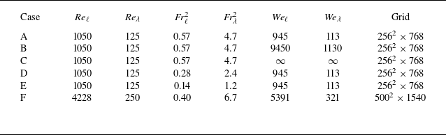The dimensionless parameters of the simulations relative to the integral and Taylor microscale ( $\lambda$ ) within the bulk forcing region are given in table 1 since those parameters are controlled. Given the nature of HIT, the r.m.s. velocity decays from the bulk to $z=-1.25 \ell$ by roughly 70 % (see Appendix A), where forcing is zero. The Taylor microscale is found to remain nearly constant with depth, hence, the Taylor scale Froude number near the free-surface is still of order unity, and can be considered moderate FST. For all cases, the density and viscosity ratios of air–water are considered: $\rho _2 / \rho _1 = 833.3$ , $\mu _2 / \mu _1 = 55.2$ . The grid is uniform and is of the same order of magnitude as the Kolmogorov scale $\eta = (\nu ^3 / \varepsilon )^{1/4}$ . The baseline grid has $256^2 \times 768$ points, with a refined grid in case F where ${\textit{Re}}$ is increased. While the variation in ${\textit{Re}}$ is limited due to computational costs, to the author’s knowledge the present DNS are the highest ${\textit{Re}}$ number isotropic FST flow to date with a deformable interface and air entrainment. The grid sizes are sufficient to capture all the relevant scales of turbulence and velocity gradients that reach the free-surface, from different metrics shown in the following sections. Statistics on entrained bubbles are shown in § 3, showing good agreement with expected scalings. The grid Weber number, ${\textit{We}}_{\Delta h}=(\rho _1+\rho _2)|u|^2\Delta h /(4 \pi \sigma )$ (Popinet Reference Popinet2018), for all cases except C ( ${\textit{We}}=\infty$ ) is calculated to be of order 1 or less, with a local velocity scale evaluated at $z=0$ . A snapshot rendering from the DNS showing the turbulent free-surface can be seen in figure 1(b).

Table 1.

Summary of free-surface turbulence DNS cases.

Figure 1.

(a) Schematic view of the domain for the subsurface turbulence generation showing damping and bulk forcing regions. Mean free-surface is at $z=0$ . The profile on the right represents the spatial forcing function $f(z_p)$ . (b) Direct numerical simulation rendering of the turbulent free-surface.

For the analysis of the flow field data, we perform ensemble averaging over uncorrelated snapshots in time (one large eddy turnover time apart). A total of 10 snapshots are used, once the flow has reached a statistical steady state. Sensitivity of the number of snapshots used in the ensemble averaging has been verified in previous works (see Calado et al. Reference Calado, Yildiran and Balaras2025) and is shown in Appendix A. Unless otherwise specified, we define the averaging operator $\langle \boldsymbol{\cdot }\rangle$ as denoting ensemble averages over the horizontal plane in the water phase. As proposed by Brocchini & Peregrine (Reference Brocchini and Peregrine2001a ), we can define an intermittency function $\gamma$ based on the average volume fraction of water. We first define the Eulerian phase function, $I(\boldsymbol{x},t)$ ,

(2.6) \begin{equation} I(\boldsymbol{x},t)=\left \{ \begin{array}{@{}ll@{}} 1 & \textrm {in water}, \\ 0 & \textrm {in air}, \\ \end{array}\right . \end{equation}

and through the averaging operator we obtain $\gamma (z) = \langle I(z) \rangle$ , as well as the intermittency layer, $\delta _i$ , where $0 \lt \gamma \lt 1$ .

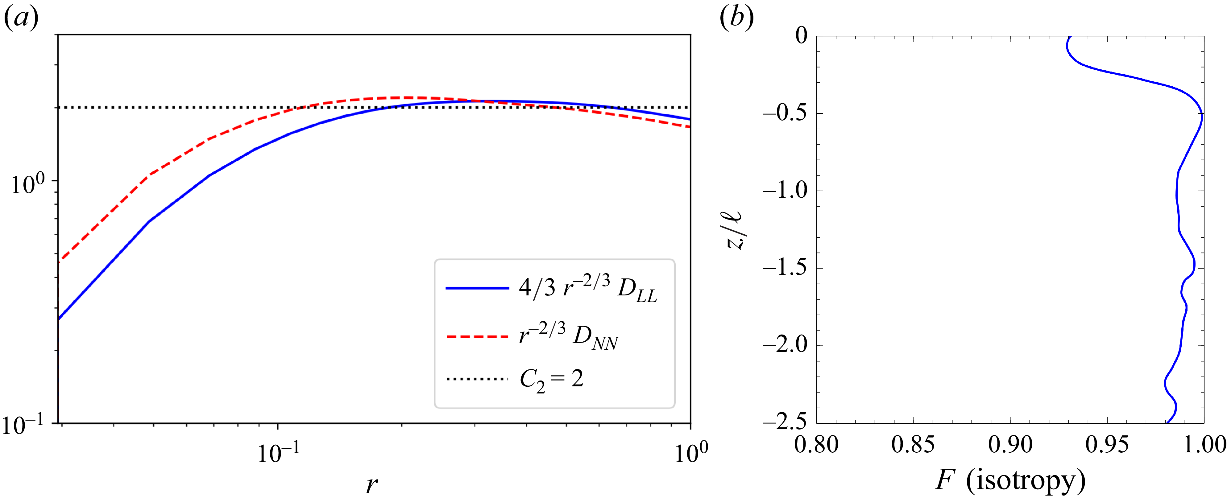
The generated turbulence in the bulk is verified to be isotropic by analysing different metrics: in figure 2(a) we plot the pre-multiplied longitudinal and transverse second-order structure functions ( $D_{\textit{LL}}$ and $D_{\textit{NN}}$ ), which exhibit a plateau around the constant $C_2 = 2.0$ in the inertial range (Pope Reference Pope2000). In addition, the level of isotropy as a function of the depth, $z$ , is quantified in figure 2(b) with the isotropy scalar, $F$ , which is bounded between 0 and 1 (pure isotropy):

(2.7) \begin{equation} F(z) = \frac {27 \langle u'^2 \rangle \langle v'^2 \rangle \langle w'^2 \rangle }{( \langle u'^2 \rangle + \langle v'^2 \rangle + \langle w'^2 \rangle )^3}. \end{equation}

We observe that the turbulence is indeed isotropic, with $F \gt 0.9$ within the bulk and damping regions, $z/\ell \lt -1.25$ , and for the selected case A, it remains isotropic until almost $z=0$ .

Figure 2.

(a) Pre-multiplied longitudinal and transverse second-order structure functions in the bulk turbulence region. (b) Phase-averaged isotropy scalar $F$ as a function of depth. Data are for case A.

4.1. Surface deformation

In the case of a quasi-flat free-surface, a linear dependency of the vertical velocity component is expected around $z=0$ such that $w(z) \sim z \partial _z w$ (McKenna & McGillis Reference McKenna and McGillis2004; Lovecchio et al. Reference Lovecchio, Zonta and Soldati2015). This also implies that the surface divergence can be evaluated as $\boldsymbol{\nabla \!} _\bot \boldsymbol{\cdot }\boldsymbol{u} = \partial _x u + \partial _y v = - \partial _z w$ , and the local sign and magnitude can indicate the presence of upwelling or downwelling structures (Longuet-Higgins Reference Longuet-Higgins1996; Babiker et al. Reference Babiker, Bjerkebaek, Xuan, Shen and Ellingsen2023). This definition however is not valid for larger ${\textit{Fr}}$ and ${\textit{We}}$ where surface deformations are appreciable (nonlinear), as seen, for example, in figure 4. The orientation of the free-surface is quantified by plotting the distribution of its normal vector components in figure 5(a) for the lowest ${\textit{Fr}}$ number case (E): it is evident that the $x$ and $y$ components are symmetrically distributed around zero and that $n_z$ is dominant. Comparing the vertical component $n_z$ for the different ${\textit{Fr}}$ we considered (see figure 5 b), we observe that even though $n_z \approx 1$ is most common, the distribution tends to be flatter indicating that the horizontal components become more relevant as the free-surface becomes increasingly deformed. Hence, we propose that the surface divergence be evaluated using the 3-D normal vector as

(4.1) \begin{equation} \boldsymbol{\nabla \!} _\bot \boldsymbol{\cdot }\boldsymbol{u} = n_x \partial _x u + n_y \partial _y v + n_z \partial _z w. \end{equation}

Figure 5.

(a) The PDF of free-surface normal components for case E, (b) PDF of $n_z$ for different ${\textit{Fr}}$ , and (c) PDF of $(\boldsymbol{\nabla \!} _\bot \boldsymbol{\cdot }\boldsymbol{u})^2$ and $\omega _z^2$ , scaled by r.m.s., for case E.

An alternative metric indicative of the deformation of the interface is related to the net stretching of the interface by the strain rate tensor $\boldsymbol{S}=(\boldsymbol{\nabla }\boldsymbol{u}+ \boldsymbol{\nabla }\boldsymbol{u}^{\top })/2$ introduced by Vela-Martín & Avila (Reference Vela-Martín and Avila2021), and written out in Cartesian coordinates as

(4.2) \begin{align} {\vartheta } &= -\boldsymbol{n}^\top \boldsymbol{\cdot }\boldsymbol{S} \boldsymbol{\cdot }\boldsymbol{n} \nonumber\\ &= n_x^2 \partial _x u + n_y^2 \partial _v + n_z^2 \partial _z w + n_x n_y (\partial _y u + \partial _x v) + n_x n_z (\partial _x w + \partial _z u) + n_y n_z (\partial _y w + \partial _z v) .\end{align}

This surface energy increase from net stretching $\vartheta \gt 0$ (or $\vartheta \lt 0$ in the case of compression) is scaled by the surface tension coefficient or ${\textit{We}}$ number as $\hat {\vartheta } = \vartheta / \textit{We}$ . The total energy being absorbed or released from the interface is thus proportional to $\varPsi _\sigma \propto - \int _\varGamma \hat {\vartheta } d\varGamma$ and can also be related to the rate of change of total interfacial area (see Dodd & Ferrante Reference Dodd and Ferrante2016; Calado & Balaras Reference Calado and Balaras2024a ). The resemblance between (4.1) and (4.2) is clear, although $\vartheta$ is introduced in the more general context of surface energy calculation for multiphase flows. In figure 5(c) we also observe that $(\boldsymbol{\nabla \!} _\bot \boldsymbol{\cdot }\boldsymbol{u})^2$ and $\omega _z^2$ at the free-surface exhibit a power law tail for small values, attributed to a chi-squared type distribution where small velocity gradients acts as random variables, highlighted in the experiments of Qi, Li & Coletti (Reference Qi, Li and Coletti2025). These variables involve a single squared term, resulting in $\beta = 1$ degrees of freedom, and a $\beta /2-1=-1/2$ scaling.

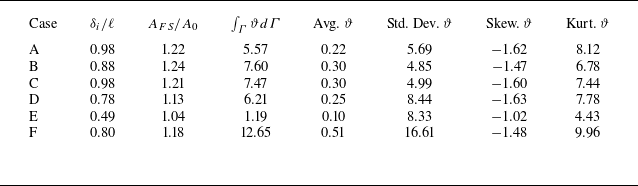
Ensemble-averaged statistics for the free-surface are presented in table 2. We compute different quantities that reflect the extent of deformation experienced by the free-surface for the different cases. These include the intermittency layer $\delta _i$ , the ratio of total free-surface area $A_{FS}$ with initial flat surface area $A_0 = L^2$ and the surface integral $\int _{\varGamma } \vartheta d\varGamma$ indicating the net stretching effect. The PDF for $\vartheta$ is characterised in terms of the mean, standard deviation, skewness and kurtosis.

Table 2.

Ensemble statistics for free-surface deformation.

Figure 6.

Comparison of free-surface contours for different surface deformation metrics for a snapshot of case E. Results are shown for (a) $- \partial _z w$ , (b) $\boldsymbol{\nabla \!} _\bot \boldsymbol{\cdot }\boldsymbol{u}$ and (c) $\vartheta$ .

We observe that the free-surface statistics are comparable between cases A, B and C, with a relative increase in surface area around $\sim\! 20 \,\%$ and weakly dependent on ${\textit{We}}$ . Note that, for this problem, since ${\textit{Fr}}^2 \ll \textit{We}$ , it is gravity that dominates the interfacial dynamics at larger scales, even though these three cases are considered to be in the moderate FST regime $(\textit{Fr}^2_{\lambda } \sim \mathcal{O}(1))$ as shown in figure 4(a), with air entrainment. The intermittency layer is found to be of the order of the integral length scale $\delta _i \sim \ell$ , although decreasing with ${\textit{Fr}}$ . Decreasing ${\textit{Fr}}$ in cases D and E shows a reduction in the total surface area and net stretching effect from $\vartheta$ , since the gravity force increases that stabilises any disruptions from the free-surface. Finally, for the high- ${\textit{Re}}$ case F, the total surface area is comparable to cases A and D, given the similar integral scale ${\textit{Fr}}^2_{\ell }$ , which determines the large-scale deformation. On the other hand, the statistics for the mean and variance of $\vartheta$ are much higher, indicative of higher velocity gradients at the interface, and smaller $\lambda$ .

Finally, we comment on the fact that all cases show a negative skewness and high kurtosis (super-Gaussian) for $\vartheta$ , which indicate large tails, with more extreme values of $\vartheta \lt 0$ , or compression. These are associated with the ridges seen in figure 6 that are thin and elongated, compared to regions of upwelling where $\vartheta \gt 0$ . As also observed by Longuet-Higgins (Reference Longuet-Higgins1996), the regions of downwelling have signature steeper waves and they surround smoother regions of upwelling. This can be tied to the upwelling versus downwelling events and their energy. Ruth & Coletti (Reference Ruth and Coletti2024) pointed out that downwellings compress energy to small scales and are less energetic compared to upwellings, which are associated with larger scales. Our results for the TKE exchange near the free-surface are presented in § 5.

4.2. Two-dimensional compressibility

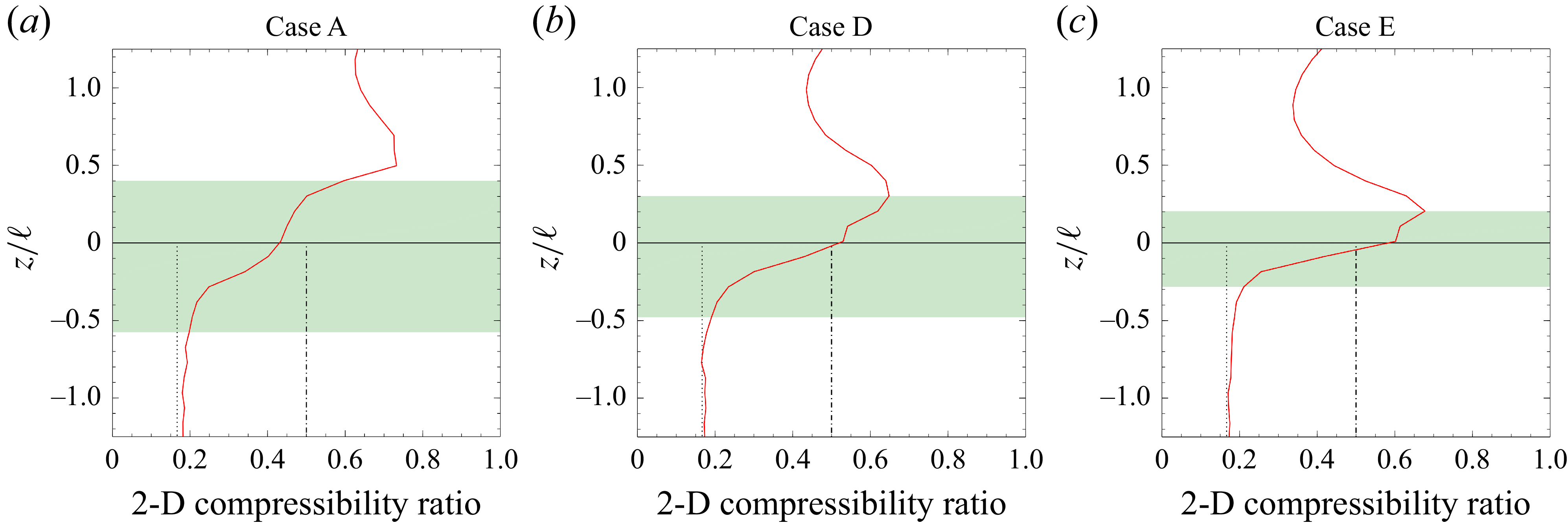
Another measure of the free-surface dynamics is the Eulerian compressibility ratio that can take values between 0 and 1. The compressibility effect can be linked to the directionality of the energy transfer (Chertkov, Kolokolov & Vergassola Reference Chertkov, Kolokolov and Vergassola1998; Lovecchio et al. Reference Lovecchio, Zonta and Soldati2015) and in free-surface flows results in Lagrangian particle clustering (Boffetta et al. Reference Boffetta, Davoudi, Eckhardt and Schumacher2004). By definition this factor is zero in three-dimensional (3-D) incompressible flows, however, in the case of homogeneous flow in the plane, this ratio can be computed in two dimensions as

(4.3) \begin{equation} \mathcal{C} = \frac {\left\langle (\boldsymbol{\nabla}_{\kern-1.5pt \textit{xy}} \boldsymbol{\cdot }\boldsymbol{u})^2 \right\rangle }{\langle |\boldsymbol{\nabla}_{\kern-1.5pt \textit{xy}} \boldsymbol{u}|^2 \rangle } = \frac {\left\langle (\partial _x u + \partial _y v)^2 \right\rangle }{ \left\langle (\partial _x u)^2 + (\partial _x v)^2 + (\partial _y u)^2 + (\partial _y v)^2 \right\rangle }. \end{equation}

Note that in this definition we consider a continuous velocity field and ignore phase distribution. A two-dimensional (2-D) cut through 3-D HIT results in an asymptotic value of $\mathcal{C} = 1/6$ , while values close to $1/2$ are observed near the free-surface in low ${\textit{Fr}}$ number experiments and DNS with a slip wall boundary condition (Cressman et al. Reference Cressman, Davoudi, Goldburg and Schumacher2004; Lovecchio et al. Reference Lovecchio, Zonta and Soldati2015). The value of $\mathcal{C}=1/2$ is also the theoretical limit for compressible 2-D Kraichnan flow (Chertkov et al. Reference Chertkov, Kolokolov and Vergassola1998) and also implies a null cross-correlation for $\langle \partial _xu \, \partial _y v \rangle$ (Boffetta et al. Reference Boffetta, Davoudi, Eckhardt and Schumacher2004). Results from our DNS are given in figure 7 for different ${\textit{Fr}}$ numbers. We observe a similar behaviour to previous studies, with an increasing value of $\mathcal{C}$ from $1/6$ in the pure water depths to $\mathcal{C} \approx 1/2$ at $z=0$ . Since data from the air side is also available, we plot the values for $z\gt 0$ , indicating a continued increase until the upper limit of $\delta _i$ is reached. As the ${\textit{Fr}}$ number is decreased, the value of $\mathcal{C}$ at $z=0$ decreases, with a stronger inflection for the highest ${\textit{Fr}}$ case. This shows that as turbulence becomes stronger, the apparent 2-D compressibility drops in magnitude while $\delta _i$ grows.

Figure 7.

Two-dimensional compressibility ratio $\mathcal{C}$ as a function of depth. The green shaded region indicates the intermittency layer $\delta _i$ ; vertical lines are shown for $\mathcal{C}=1/6$ (dotted) and $\mathcal{C}=1/2$ (dash-dotted). (a) Case A (b) Case D (c) Case E.

4.3. Vorticity alignment

In an incompressible interfacial flow, the only mechanism to generate vorticity is the inviscid relative acceleration between fluids due to tangential pressure gradients or body forces (see Terrington et al. Reference Terrington, Hourigan and Thompson2022b ). Surface normal vorticity can appear either from advection across the interface or from viscous diffusion of tangential vorticity. This leads to the attachment of vortex filaments to the free-surface, such that the kinematic condition is satisfied (vortex filaments do not end inside a fluid). The no-slip condition between two fluids imposes the normal vorticity component to be continuous, while the tangential components are related to the interface curvature (Dopazo, Lozano & Barreras Reference Dopazo, Lozano and Barreras2000).

Ignoring the absolute value in the sign of vorticity, we compute the averages of squared vorticity components, $\langle \omega _i^2 \rangle$ , and plot them in figure 8(a) for case A. Note that these averages are not phase averaged. The vorticity is seen to be isotropic below $z/\ell \lt -0.5$ , with a change in behaviour approaching $z=0$ , with an inflection for all components, and a stronger increase in horizontal components. This was seen consistently in all cases, although as ${\textit{Fr}}$ decreases, the increase in the vertical component $\omega _z$ is negligible. The vorticity alignment with the free-surface can be evaluated using the dot product between the vorticity $\boldsymbol{\omega } = \boldsymbol{\nabla }\times \boldsymbol{u}$ and the normal vector (Mukherjee et al. Reference Mukherjee, Safdari, Shardt, Kenjereš and Akker2019; Vela-Martín & Avila Reference Vela-Martín and Avila2021; Cannon, Soligo & Rosti Reference Cannon, Soligo and Rosti2024):

(4.4) \begin{equation} \textrm {cos}(\theta _{\omega }) = \frac {\boldsymbol{n}\boldsymbol{\cdot }\boldsymbol{\omega }}{|| \boldsymbol{\omega } ||}. \end{equation}

Plotting the PDF of this function shows a symmetric distribution around $\textrm {cos}(\theta _\omega ) = 0$ that can be approximated by a Laplacian distribution $\mathcal{L} (x|s) = \textrm {exp}( - |x|/s)/(2s)$ with scale parameter $s=0.3$ , as seen in figure 8(b). Using this model, Laplacian distribution equates to $\sim\! 80 \,\%$ probability for the angle $\theta _\omega$ being greater than $60^\circ$ . This distribution was also found to be weakly dependent on ${\textit{Fr}}$ and ${\textit{We}}$ . These results indicate that the vorticity is mainly oriented parallel to the free-surface, in agreement with other works for free-surface and disperse two-phase flows (Sarpkaya Reference Sarpkaya1996; André & Bardet Reference André and Bardet2017; Yu et al. Reference Yu, Hendrickson, Campbell and Yue2019; Masnadi et al. Reference Masnadi, Erinin, Washuta, Nasiri, Balaras and Duncan2020; Vela-Martín & Avila Reference Vela-Martín and Avila2021; Calado & Balaras Reference Calado and Balaras2024a ). We observe that the case with the lowest ${\textit{Fr}}$ number has some differences at the tails, indicating a higher likelihood for vortices to connect normal to the interface due to stronger gravity and a flatter interface.

Figure 8.

(a) Squared vorticity components (non-phase averaged) normalised by values at $z/\ell =-1.25$ for case A, (b) PDF of $\textrm {cos}(\theta _\omega )$ for different ${\textit{Fr}}$ and Laplacian distribution.

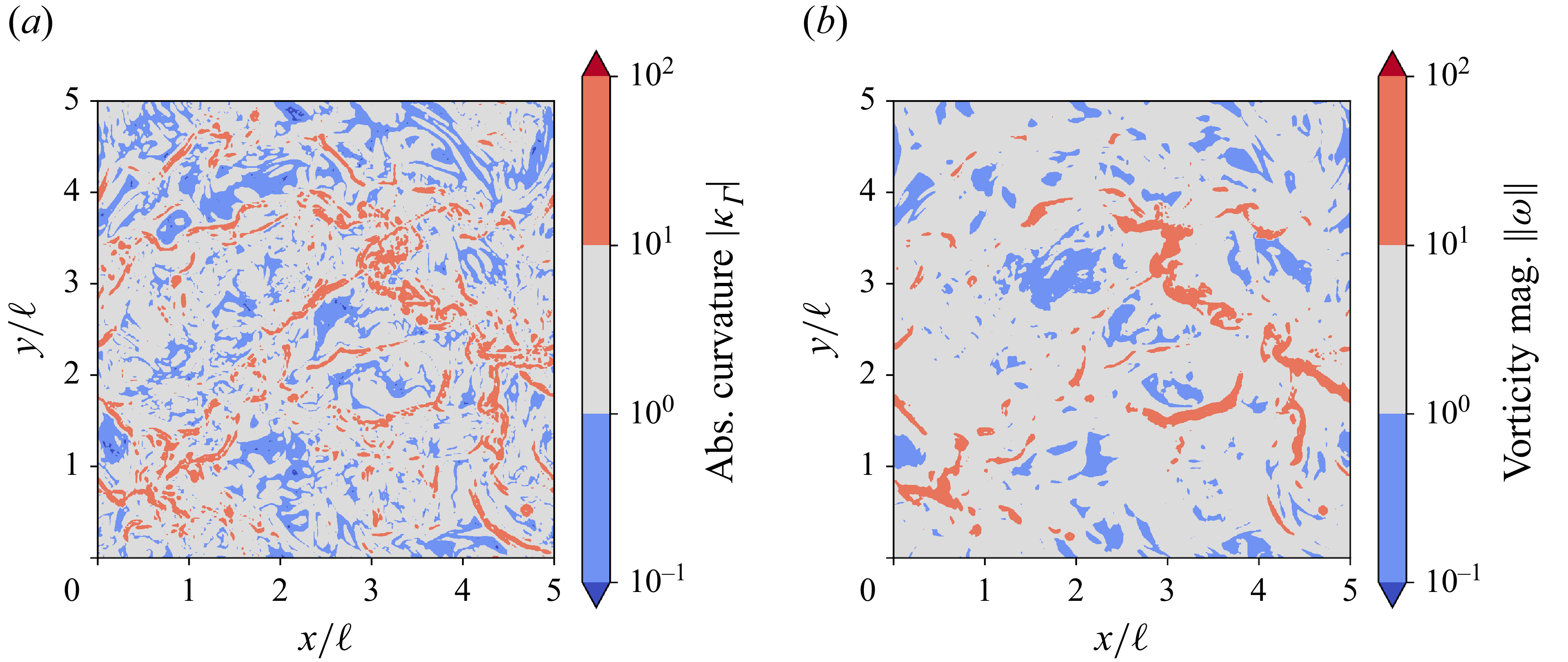
Comparing the plots of the absolute value for interface curvature $| \kappa _\varGamma |$ and the vorticity magnitude $|| \boldsymbol{\omega }||$ on a logarithmic scale in figure 9, we can observe that regions of high curvature form continuous streaks or scars, which is a characteristic signature of free-surface flows (Brocchini & Peregrine Reference Brocchini and Peregrine2001b ). The vorticity magnitude is seen to be highly correlated with the absolute value of curvature. From these plots and the observed distributions of $\theta _\omega$ , we can infer that most of the vorticity flux across the free-surface is attributed to the viscous diffusion of tangential vorticity (Dopazo et al. Reference Dopazo, Lozano and Barreras2000; Terrington et al. Reference Terrington, Hourigan and Thompson2022a , Reference Terrington, Hourigan and Thompson2022b ). This is clearly visualised in figure 10 by plotting $Q = (||\boldsymbol{\varOmega }||^2_F - ||\boldsymbol{S}||^2_F)/2$ criterion ( $Q\gt 0$ ) isosurfaces near the free-surface, where $\boldsymbol{\varOmega }=(\boldsymbol{\nabla }\boldsymbol{u}- \boldsymbol{\nabla }\boldsymbol{u}^{\top })/2$ is the rotation rate tensor and $|| \boldsymbol{\cdot }||^2_F$ is the Frobenius norm squared. We choose case F specifically for this visualisation given the greater grid resolution, although results are similar for other cases. Within roughly one integral length scale (blockage layer), the vortices transition from randomly oriented in the bulk, towards being parallel to the free-surface.

Figure 9.

Snapshot contour maps of the free-surface on a log scale for (a) the absolute interface curvature and (b) the vorticity magnitude. Data refers to case A.

Figure 10.

The $Q$ criterion isosurfaces above $z/\ell \gt -1.25$ , coloured by distance to the interface for case F. Only a limited number of the largest structures are shown for clarity.

5.1. Reynolds stresses

First we look at the Reynolds stress components near the free-surface and how they are modulated by the ${\textit{Fr}}$ number. In figure 11 we compare the vertical fluctuating velocities for different ${\textit{Fr}}$ numbers to RDT predictions. Note that $\langle w^{\prime}_{\textit{rms}} \rangle \propto (|z| + \delta _v)^{1/3}$ , with $\delta _v \approx 4 Re_{\ell }^{-1/2}$ (Hunt & Graham Reference Hunt and Graham1978; Variano & Cowen Reference Variano and Cowen2008). The vertical component $\langle w^{\prime}_{\textit{rms}}\rangle$ is seen to agree well with the trend from RDT at lower ${\textit{Fr}}$ numbers. Potential discrepancies here can be tied to the moderate ${\textit{Re}}$ number, since RDT is based on the inviscid assumption (see Ruth & Coletti Reference Ruth and Coletti2024). The horizontal components are seen to remain higher than vertical components, particularly for the lower ${\textit{Fr}}$ numbers where blockage effects are increased. We also note an inflection point above the viscous layer $\delta _v$ .

Figure 11.

The r.m.s. velocities for different ${\textit{Fr}}$ numbers for the (a) vertical component and (b) horizontal component. Data normalised by values at $z/\ell =-1.25$ .

Figure 12.

Lumley triangle plot for case A (red circles) and case E (blue triangles) for $-1.25 \leqslant z \leqslant 0$ . The darker hue of the crosses corresponds to depths approaching $z=0$ .

The variation in Reynolds stress components can alternatively be visualised by plotting the Lumley triangle as a function of depth (Pope Reference Pope2000; Yu et al. Reference Yu, Hendrickson, Campbell and Yue2019). Starting from the normalised anisotropy tensor $b_{\textit{ij}} = {\langle u_i u_j \rangle } / {\langle u_k u_k \rangle }- 1/3 \delta _{\textit{ij}}$ we compute the two independent tensor invariants $\chi$ and $\xi$ , defined as $ \chi = (b_{\textit{ij}}b_{\textit{ji}} / 6)^{1/2}$ and $\xi = (b_{\textit{ij}}b_{jk}b_{ki} / 6)^{1/3}$ . The cases of lowest and highest ${\textit{Fr}}$ numbers (A and E) are plotted in figure 12 for depths between $z/\ell =-1.25$ and $z=0$ . The isolines of $F=0.6$ and $F=0.9$ are also plotted for reference. We clearly see that in case A (higher ${\textit{Fr}}$ ), the isotropy is maintained as the depth is decreased, with $F\gt 0.9$ . However, as ${\textit{Fr}}$ is decreased in case E, the turbulence is modulated from isotropic to two-component axisymmetric, due to the increase in horizontal energy at the expense of vertical fluctuations. These results oppose the postulation by Sarpkaya (Reference Sarpkaya1996) that any turbulence field approaching a free-surface becomes two dimensional. While this is certainly the case for lower ${\textit{Fr}}$ numbers, the turbulence tends to remain isotropic with higher ${\textit{Fr}}$ since there is a reduced blockage effect.

Figure 13.

Instantaneous horizontal slice of $w'|w'|$ for depths $z/\ell =-2.5$ (a) and $z/\ell =-1$ (b) for case A. Conditionally averaged statistics for vertical kinetic energy based on sign, normalised by values at $z/\ell =-2.5$ for case A (c); ratio of upwelling to downwelling energy for cases A and E (d).

Another relevant question investigated by Ruth & Coletti (Reference Ruth and Coletti2024) is the relative roll of upwellings versus downwellings in transporting vertical kinetic energy. In the low ${\textit{Fr}}$ number cases investigated in their work, they found that upwellings carry more vertical energy, while downwellings move more horizontal energy due to compressive effects from the free-surface. We investigate these statistics by conditionally averaging the vertical energy, $\langle w'^2 \rangle$ , based on its sign: $w' \gt 0$ for upwellings and $w' \lt 0$ for downwellings. An instantaneous snapshot of $w'|w'|$ on horizontal slices at depths of $z/\ell =-2.5$ and $z/\ell =-1$ in figures 13(a) and 13(b), respectively, also support this fact ( $w'|w'|$ indicates both the magnitude of kinetic energy and its relative motion). Quantitative results are given in figure 13(c) on a semi-log scale and show qualitative agreement with the experiments of Ruth & Coletti (Reference Ruth and Coletti2024). In figure 13(d) we compute the ratio of upwelling energy to downwelling energy $\langle w'^2\rangle ^{+} / \langle w'^2\rangle ^{-}$ for cases A and E, showing a higher ratio for larger ${\textit{Fr}}$ at depths within the blockage layer. For greater depths, the turbulence does not sense the influence of the free-surface, and kinetic energy is transported equally in both vertical directions, while within the blockage layer, $\delta _s$ , the upwellings bring the necessary energy to stretch out the free-surface. Within the viscous layer $\delta _v$ this ceases to be true and vertical energy tends to recover isotropy.

5.2. Presence of upscale transfer

The third-order structure function is useful to determine the cascading direction of TKE. In particular, its sign indicates either a forward ( $-$ ) or reverse ( $+$ ) energy cascade at the specific length scale $r$ (Lovecchio et al. Reference Lovecchio, Zonta and Soldati2015; Ruth & Coletti Reference Ruth and Coletti2024). According to the Kolmogorov $4/5$ law, the archetypal cascade for HIT compresses energy from large to small scales within the inertial subrange, reflected in a negative third-order structure function (Pope Reference Pope2000). Following Ruth & Coletti (Reference Ruth and Coletti2024) we define the TKE in the $i$ component of velocity difference between two points $q_i = \Delta u_i (\boldsymbol{x},\boldsymbol{r})^2 = [u_i(\boldsymbol{x}+\boldsymbol{r})-u_i(\boldsymbol{x})]^2$ . The compression or stretching of energy is thus given by $q_i (\boldsymbol{x},\boldsymbol{r}) \Delta u_j (\boldsymbol{x},\boldsymbol{r})$ . By ensemble averaging in time and along the homogeneous horizontal direction ( $j=x,y$ ), we can define the inter-scale energy transfer rate for a separation length $r$ as a function of the vertical coordinate $\langle q_i \Delta u_j \rangle (z,r)$ . For horizontal velocity differences, $\langle q_x \Delta u_x \rangle$ equates to the longitudinal third-order structure function $D_{LLL}$ (Pope Reference Pope2000). In figure 14 we plot $\langle q_x \Delta u_x \rangle$ and $\langle q_z \Delta u_x \rangle$ for depths above $z/\ell =-1.25$ for different ${\textit{Fr}}$ numbers (cases A, D and E). Note that these statistics are computed considering the water phase only and are normalised by $\langle k \rangle ^{3/2}$ at the same depth. As a reference, we also plot the same functions for case A within the bulk HIT region.

Within the single-phase bulk region we observe the typical forward cascade (negative sign) and $\langle q_x \Delta u_x \rangle \propto -r$ within the inertial range (Pope Reference Pope2000). For case A, the difference between horizontal and vertical energy fluxes are smaller compared to lower ${\textit{Fr}}$ numbers. At greater depths the flux is still mostly negative (forward) for small scales, but much smaller in magnitude compared to the bulk. As we approach the free-surface there is evidence of upscale energy transfer above $r/\ell \sim 0.1-0.2$ and below which the flux is close to zero, indicative of a bi-directional energy transfer (i.e. forward and reverse). Pan & Banerjee (Reference Pan and Banerjee1995) also investigated the inter-scale energy transfer from spectral analysis and verified that at large scales both significant forward and reverse transfer can occur (although net forward), while for smaller scales (high wavenumbers), magnitudes are comparable, yielding roughly net zero exchange. For cases D and E, with the reduction in ${\textit{Fr}}$ the upscale energy exchange is only evident for the vertical component, $\langle q_z \Delta u_x \rangle$ . Results for the lowest ${\textit{Fr}}$ case show qualitative agreement with Ruth & Coletti (Reference Ruth and Coletti2024), which also showed $\langle q_z \Delta u_x \rangle \gt 0$ near the free-surface, as evidence of the upscale transfer effect. Finally, we plot both $\langle q_x \Delta u_x \rangle$ and $\langle q_z \Delta u_x \rangle$ as a function of depth for $r/\ell =0.5$ . We also indicate $\delta _i$ in the shaded green region, where $\gamma$ drops rapidly from 1 to $0.5$ at $z=0$ , potentially affecting the phase-averaged statistics in this layer. The trends are consistent across cases in that the vertical motions are more prone to an upscale energy transfer at these larger scales, relative to horizontal ones. The presence of the free-surface inhibits the forward/downscale transfer by limiting compression and favouring horizontal stretching due to the more energetic upwellings. Statistics for the inter-scale energy transfer function were found to be similar between cases A and F at higher ${\textit{Re}}$ . Note that these metrics are relative to specific components of the kinetic energy along the horizontal direction and that net TKE flux at the same depth can still remain downscale as described in Pan & Banerjee (Reference Pan and Banerjee1995). While these functions indicate upscale energy transfer at larger scales near the interface, this does not necessarily demonstrate scale locality for a cascade process, where energy would transfer gradually between adjacent scales. Vortex mergers may contribute to non-local effects and future work is needed to quantify the degree of locality in these flows. We also observe that entrained bubbles have a radius below $r/\ell \lt 0.1$ , where a downscale transfer is observed.

Figure 14.

Inter-scale energy transfer as a function of depth and horizontal separation: (ac) horizontal TKE and (df) vertical TKE; (gi) vertical and horizontal components for $r=0.5 \ell$ , with $\delta _i$ shaded in green. Cases are A, D and E from left to right (decreasing ${\textit{Fr}}$ ). The red solid line represents transfer in the bulk HIT region for reference.

5.3. Energy spectra

To complement the quantitative analysis of the different components of TKE and at which length scales they are present, we compute the traditional one-dimensional (1-D) Fourier spectra at a fixed depth in the water phase. In figure 15 we compare the horizontal $(E_{uu})$ and vertical $(E_{ww})$ velocity power spectral density (PSD) for cases A and E at different ${\textit{Fr}}$ numbers at the same $z/ \ell =-0.25$ . Similar to the results from the Lumley plot (figure 12), we observe that case A has higher isotropy since the PSDs are comparable, and follow the $\tilde {k}^{-5/3}$ law characteristic of the inertial subrange. Case E (lower ${\textit{Fr}}$ ) shows a higher magnitude for $E_{uu}$ relative to $E_{ww}$ for the lowest wavenumbers that are the most energetic. For mid and high wavenumbers, the PSD is comparable, indicating that anisotropy is mostly associated with the largest scales. In addition, a steeper decay in energy is noted for the lower ${\textit{Fr}}$ case (E) relative to case A; similar trends are also reported in the literature (Yu et al. Reference Yu, Hendrickson, Campbell and Yue2019; Jamin et al. Reference Jamin, Berhanu and Falcon2025). A transition from a −5/3 to −3 slope is observed in case A, which is also reported in the DNS and experiments of Pan & Banerjee (Reference Pan and Banerjee1995) and Kumar & Banerjee (Reference Kumar and Banerjee1998) and is attributed to a quasi-2-D behaviour and reverse energy cascade. While the change in slope for the energy spectrum is also observed for bubble-induced turbulence (see Lance & Bataille Reference Lance and Bataille1991; Bunner & Tryggvason Reference Bunner and Tryggvason2002; Roghair et al. Reference Roghair, Mercado, Annaland, Kuipers, Sun and Lohse2011; Prakash et al. Reference Prakash, Mercado, Wijngaarden, Mancilla, Tagawa, Lohse and Sun2016) in our case, the underlying physics are quite different. For instance, in case E there are no entrained air bubbles below the surface.

Figure 15.

Fourier PSD of kinetic energy components of the water phase at $z/\ell =-0.25$ for different ${\textit{Fr}}$ . (a) Case A (b) Case E.

A limitation of the traditionally used 1-D spectral analysis is that it does not differentiate between phases if used naively, and is agnostic of interface proximity. Even though the velocity field is continuous across the interface, mismatching viscosities imposes discontinuous velocity gradients that can contribute to additional energy content in the higher wavenumbers. One alternative that offers local information based on the phase or distance to the interface uses wavelets to compute the spectral energy. This is known as a phase-based wavelet analysis and has been used in recent works by Freund & Ferrante (Reference Freund and Ferrante2019) and Calado & Balaras (Reference Calado and Balaras2024a ). 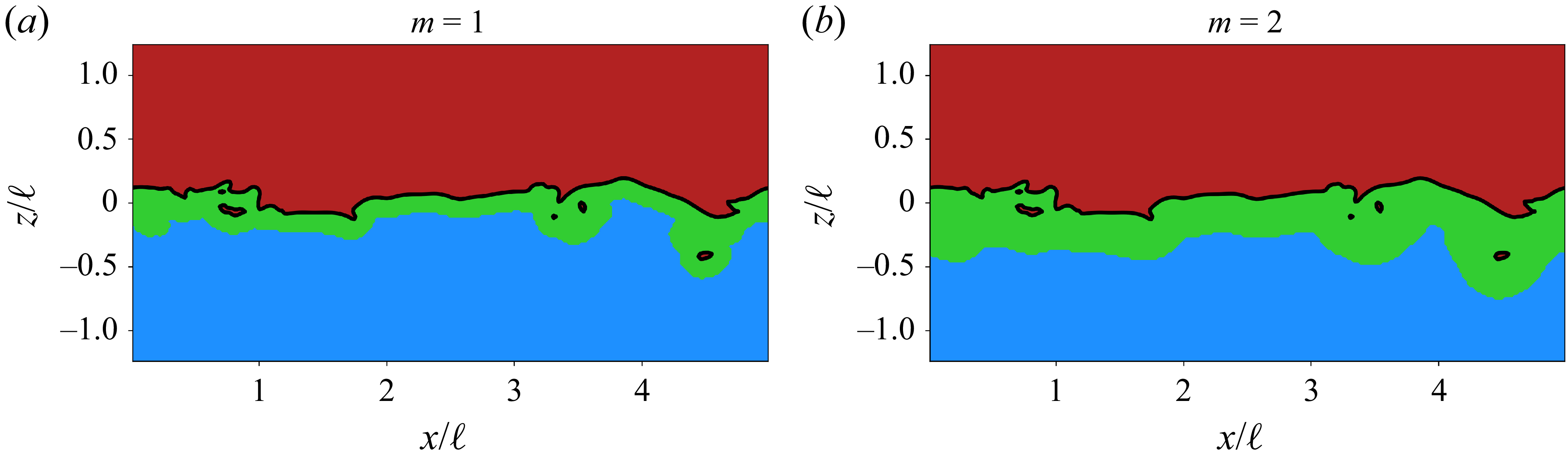For the sake of completeness, we include a brief description of this approach and refer to the cited references for more details. The method starts by decomposing the physical domain into three subsets based on the distance to the interface, $\phi$ , defining liquid, gas and interfacial subsets as $\mathcal{D}_L, \mathcal{D}_G$ and $\mathcal{D}_I$ , respectively. Due to the high density ratio, the kinetic energy associated with the air phase is negligible, and the interfacial subset only includes the neighbouring region in the water side. A multi-resolution DWT of the 3-D velocity field can be performed for a range of scales $1 \leqslant m \leqslant M$ , from smallest $(m=1$ ) to largest $m=M$ . The wavelet order determines the smallest scale and doubles progressively until the largest scale, $M=\textrm {log}_2(N)$ , which depends on the domain size. In our case, we take the horizontal domain size $L$ . The equivalent wavenumber is given by $\tilde {k}_m= 2 \pi / (2^m \Delta h)$ . Following previous works (Freund & Ferrante Reference Freund and Ferrante2019; Calado & Balaras Reference Calado and Balaras2024a ) we use the fourth-order Symlet wavelet family (orthogonal and of compact support), using eight points in each spatial direction for $m=1$ . The domain decomposition can be readily performed based on the level-set function $\phi$ and the scale-dependent threshold distance. A discrete wavelet family of order $p$ has $n_p=2p$ points for $m=1$ . The threshold distance for each scale is computed as $\tilde {\phi }^{(m)} = 2^{(m-1)} n_p \Delta h$ . Hence, the interfacial region $\mathcal{D}_I^{(m)}$ is defined for $ - \tilde {\phi }^{(m)} \leqslant \phi \leqslant 0$ . An example of this can be seen in figure 16 for scales $m=1$ and $m=2$ . Note that the interfacial domain will capture the region in the vicinity of the free-surface, as well water droplets and surrounding entrained bubbles for higher ${\textit{Fr}}$ number cases. Nonetheless since the total interfacial area is dominated by the free-surface, the influence of disperse bubbles/droplets is negligible for the overall near surface dynamics. The PyWavelets package is used to compute the wavelet coefficients from the DNS data with the spectra being ensemble averaged over the different snapshots in time (Lee et al. Reference Lee, Gommers, Waselewski, Wohlfahrt and O’Leary2019). We note that while comparisons with traditional Fourier spectra could be made, the DWT brings additional degrees of freedom, where in three dimensions it considers all possible combinations of linear, planar and volumetric dilatations (see, for example, Meneveau Reference Meneveau1991). Furthermore, since the wavelet coefficients are averaged over subdomains based on the distance from the interface, it is not restricted to low ${\textit{Fr}}$ cases or cases with a small deformation of the free-surface.

Figure 16.

Slice view of example snapshot for domain subsets used in the wavelet analysis for the smallest scales. The black line represents the interface $(\phi = 0)$ . Coloured regions represent the air (red), interfacial (green) and water (blue) subsets. Data are for case A. Results are shown for (a) $m=1$ and (b) $m=2$ .

The wavelet spectra for the liquid and interfacial domains for case A are shown in figure 17(a) and are restricted to scales smaller than $L/2$ . Case A shows a higher spectral energy in the pure water phase relative to the interfacial one since it includes the bulk forcing region, and a decay approaching the $-5/3$ law. The interfacial spectra has a markedly different shape, with a −1 slope in the low frequency range and a $-3$ slope for mid-range wavenumbers. The slope changes again towards a less steep decay for the highest wavenumbers that are closest to the interface. The interfacial spectra for cases A, C and E are given in figure 17(b), exhibiting a slightly higher energy content for low wavenumbers in case E (low ${\textit{Fr}}$ ) and similar trends for mid and high wavenumbers. The weak dependence on ${\textit{We}}$ for the current parameter space is also seen here even at the smallest scales. Finally, we compare cases A and F in figure 17(c) with small differences over the wavenumber range, although the change in slope at higher $\tilde {k}_m$ is confirmed with the improved grid resolution of case F. This apparent pileup of energy at the smallest scales near the interface was confirmed by plotting the wavelet energy at $m=1$ in a contour slice and comparing against the total kinetic energy in figure 18. For all cases, we consistently observe a concentration of high energy at these smallest wavelet scales next to the interface. While surface tension is known to modulate the fluid TKE if the ${\textit{We}}$ number is low enough (see, e.g. Dodd & Ferrante Reference Dodd and Ferrante2016; Saeedipour & Schneiderbauer Reference Saeedipour and Schneiderbauer2022), we have shown in our case that the ${\textit{We}}$ number is sufficiently large such that these effects would be minimised. This suggests that the higher energy content at small scales stem from the free-surface dynamics. From the change in slope toward $-3$ in the spectra we note the transition wavenumber to be around $\tilde {k}_m \approx 20$ , which corresponds to a length scale $ \sim\! 0.3 \ell$ . The dual energy exchange discussed in § 5.2 likely plays a role in the –3 scaling of energy for scales smaller than this value as postulated by Pan & Banerjee (Reference Pan and Banerjee1995). The upper bound of the –3 slope occurs at $\tilde {k}_m \approx 80$ ( $ 0.078 \ell$ ).

Figure 17.

Wavelet spectra for case A, comparing pure water and interfacial spectra (a); interfacial spectra comparing cases A, C and E (b); cases A and F (c).

Figure 18.

Contour plots for (a) total kinetic energy and (b) the smallest wavelet scale $m=1$ near the free-surface. The interface is shown by the solid white line, while the interfacial region for $m=1$ is shown by the neighbouring white dashed line. Data are for case A.

The large-scale dynamics is governed by gravitational forces and dampened by the interface (Frederix et al. Reference Frederix, Mathur, Dovizio, Geurts and Komen2018; Freund & Ferrante Reference Freund and Ferrante2019; Saeedipour Reference Saeedipour2023). It is well known in 2-D turbulence that a change in slope from −5/3 to −3 occurs for wavenumbers larger than some forcing wavenumber, associated with a direct/forward cascade of enstrophy (Kraichnan Reference Kraichnan1971; Xiao et al. Reference Xiao, Wan, Chen and Eyink2009). Reverse or split/dual energy cascades exist in a variety of flow configurations (see Alexakis & Biferale Reference Alexakis and Biferale2018 for definitions and different examples). While the 2-D nature is imposed in some configurations, we have demonstrated that turbulence remains three dimensional for the higher ${\textit{Fr}}$ cases in the present work. In addition, under stable stratification, gravity will naturally oppose any vertical displacement of fluid, removing kinetic energy and potentially affecting the transfer mechanisms and local dissipation rates, as pointed out by Bolgiano (Reference Bolgiano1959). The PSD of the gravitational potential energy is proportional to ${E}_g \propto z^2$ and, for the values of ${\textit{Fr}}$ and ${\textit{We}}$ used in this work, it makes up almost the entirety of the total potential energy (Guo & Shen Reference Guo and Shen2010). To quantify the spectral energy associated with the free-surface elevation, we perform a mapping of the free-surface $z$ coordinate onto a bi-dimensional grid of the same resolution as the DNS. This grid data is then used to compute 1-D Fourier spectra of the elevation to measure ${E}_g$ . This is given in figure 19 for cases A, D, E and F, normalising by the energy of the first wavenumber. The data collapses and exhibits a decay with a slope of $-7/5$ for a wide range of wavenumbers. The decay however is less steep for high wavenumbers, indicating a different behaviour at small scales, except for the lowest ${\textit{Fr}}$ case (case E) that has the lowest deformations. On a relative basis, this indicates that the conversion between gravitational (potential) and kinetic energy around the free-surface is more relevant at the smallest scales.

Figure 19.

Power spectral density of the free-surface elevation for different cases, normalised by energy of the smallest wavenumber.

Another potential mechanism for the higher energy content in the vicinity of the interface stems from modulations in the local turbulence dissipation rate $\varepsilon$ . In Walker, Leighton & Garza-Rios (Reference Walker, Leighton and Garza-Rios1996) a decrease in dissipation is observed from the elimination of tangential vorticity fluctuations in a flat free-surface. While this is also the case in the local tangential directions for the deformable free-surface simulations of Guo & Shen (Reference Guo and Shen2010), they do not observe a substantial change in the dissipation rate near the interface. The behaviour in vorticity is markedly different between a flat free-surface (slip wall) and two-fluid interfaces (quasi-free-surface) as shown in § 4.3 and in Terrington et al. (Reference Terrington, Hourigan and Thompson2022a ). We analyse the depth-averaged dissipation rate $\langle \varepsilon \rangle$ in figure 20(a), along with a single-phase simulation for comparison at ${\textit{Re}}_{\lambda } = 125$ . While the decay in dissipation rate is monotonic in a single-phase case outside of the forcing region, all two-phase cases show an inflection around $z/\ell \approx -0.5$ . The higher ${\textit{Fr}}$ in case A shows less dissipation, and a similar trend is verified for case F. A snapshot of the local dissipation rate is plotted in figure 20(b) for case F, showing a sudden decay in $\varepsilon$ within the blockage layer, with local areas of higher dissipation just below the interface. This analysis of $\langle \varepsilon \rangle$ , $E_g$ and wavelet spectra shows that small scales within this distance from the interface are unable to effectively dissipate their energy from viscosity.

Figure 20.

(a) Average turbulent dissipation rate $\langle \varepsilon \rangle$ in the water phase for cases A, E, F and single-phase (SP) simulation at ${\textit{Re}}_{\lambda }=125$ for reference; data normalised by values at $z/\ell = -2.5$ ; (b) instantaneous contour slice (log scale) of $\varepsilon$ for case F.

Figure 21.

The PDF of the flow topology parameter $\varSigma$ for increasing distances from the interface $\tilde {\phi }$ and associated dissipation rate $\tilde {\varepsilon }$ (a); instantaneous contour plot of $\varSigma$ : top view $\phi =0$ (b), bottom view $\phi =0.08\ell$ (c), slice view (d).

To further characterise the flow near the interface and explore the dissipation regime, we introduce the topology parameter $ \varSigma = (||\boldsymbol{S}||^2_F - ||\boldsymbol{\varOmega }||^2_F) / (||\boldsymbol{S}||^2_F + ||\boldsymbol{\varOmega }||^2_F )$ used in Cannon et al. (Reference Cannon, Soligo and Rosti2024). This scalar parameter is bounded between $\pm 1$ and can describe states of pure rotation (−1), shear strain (0) or extensional strain (+1). We recall that only states outside of pure rotation ( $\varSigma \neq -1$ ) indicate some level of strain in the fluid parcel and contribute toward local dissipation. Focusing on the same scales analysed through the multi-scale wavelet decomposition presented previously, we compute the PDF of $\varSigma$ for distances from the interface shorter than $\sim\! \ell$ for case F (see figure 21 a). The averaged dissipation rates within these same regions were computed and given in the same graph as $\tilde {\varepsilon }$ . Through this averaging process we provide additional confirmation of the non-monotonic behaviour of the turbulent dissipation rate near the interface and the impact on the TKE exchange. For scales closest to the interface (within $\delta _v$ ), the PDF peaks close to $\varSigma \approx 1$ , indicating dominance of extensional strain occurring at the interface. This is further confirmed by plotting $\varSigma$ and taking a top view from the free-surface ( $\phi =0$ ) in figure 21(b), compared to a view from the bottom at $\phi = 0.08 \ell$ shown in figure 21(c): it is evident that within this short distance the flow changes to have regions of pure rotation. The extensional strain stems from the compression/stretching of the interface as observed in § 4.1, with large regions of net stretching and ridges with high compression. As the distance from the interface grows, the PDFs converge and shift toward smaller values of $\varSigma$ and a more uniform distribution between shear and extensional strain. Furthermore, we can see the extent of the regions associated with pure rotation and strain to grow from figure 21(d).