1. Introduction
When an external force perturbs a tubular vesicle from its equilibrium shape, the vesicle may undergo ‘pearling’, which is a phenomenon where beads spontaneously form in the vesicle’s central neck in a manner similar to the Rayleigh–Plateau instability for droplets (Tomotika Reference Tomotika1935). Since the pioneering work by Bar-Ziv & Moses (Reference Bar-Ziv and Moses1994), vesicle pearling has been observed in a wide variety of situations, including pearling induced by (a) laser tweezers (Bar-Ziv, Moses & Nelson Reference Bar-Ziv, Moses and Nelson1998), (b) electric fields (Sinha, Gadkari & Thaokar Reference Sinha, Gadkari and Thaokar2013), (c) magnetic fields (Menager et al. Reference Menager, Meyer, Cabuil, Cebers, Bacri and Perzynski2002), (d) osmotic shock (Yanagisawa, Imai & Taniguchi Reference Yanagisawa, Imai and Taniguchi2008; Sanborn et al. Reference Sanborn, Ogle, Krautb and Parikh2013), and (e) adsorption of nanoparticles and/or polymers (Lipowsky & Dobereiner Reference Lipowsky and Dobereiner1998; Tsafrir et al. Reference Tsafrir, Sagi, Arzi, Guedeau-Boudeville, Frette, Kandel and Stavans2001). These shape transitions are a consequence of the external force inducing a tension on the vesicle’s membrane. When this tension overcomes the membrane’s bending resistance, the membrane becomes linearly unstable to long-wave, axisymmetric shape perturbations (Goldstein et al. Reference Goldstein, Nelson, Powers and Seifert1996; Powers Reference Powers2010).
In this paper, we will examine pearling induced by extensional flow. This situation is different from the cases examined previously, as the vesicle is inherently in a non-equilibrium state. In fact, before pearling, a vesicle in flow extends indefinitely in a manner similar to the breakup of droplets (Kantsler, Segre & Steinberg Reference Kantsler, Segre and Steinberg2008; Narsimhan, Spann & Shaqfeh Reference Narsimhan, Spann and Shaqfeh2014). We will perform boundary integral simulations to determine the critical conditions of pearling in flow, and compare these results with recent experiments by Kantsler et al. (Reference Kantsler, Segre and Steinberg2008). We will also compare our simulations to the classical equilibrium theories that are applicable to the situations described in the previous paragraph (Goldstein et al. Reference Goldstein, Nelson, Powers and Seifert1996; Powers Reference Powers2010; Boedec, Jaeger & Leonetti Reference Boedec, Jaeger and Leonetti2014). We find that the classical theories describe the qualitative features of flow-induced pearling, but cannot quantitatively capture the critical conditions for pearling. Finite length effects and non-uniform tension created by the flow play a significant role in this instability.
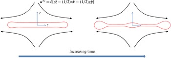
The geometry we employ is shown in figure 1. We place a vesicle in an uniaxial extensional flow, characterized by a rate of extension
 $\dot{{\it\epsilon}}$
:
 $$\begin{eqnarray}\boldsymbol{u}^{\infty }=\dot{{\it\epsilon}}[-{\textstyle \frac{1}{2}}x,-{\textstyle \frac{1}{2}}y,z].\end{eqnarray}$$
Geometry of vesicle undergoing pearling: we place an equilibrium vesicle in a uniaxial extensional flow, and monitor the deformation over time. Details of the simulation are in § 2.

Above a critical extension rate
 $\dot{{\it\epsilon}}_{b}$
, the vesicle stretches indefinitely in a manner similar to droplet breakup. This‘burst’instability has been characterized experimentally by Kantsler et al. (Reference Kantsler, Segre and Steinberg2008) and theoretically/computationally by Narsimhan et al. (Reference Narsimhan, Spann and Shaqfeh2014). At even higher extension rates, the vesicle undergoes a pearling transition, characterized by another critical condition
 $\dot{{\it\epsilon}}_{c}$
. We determine
 $\dot{{\it\epsilon}}_{c}$
by calculating the shape of the vesicle as a function of time. We assume the flow around the vesicle is at zero Reynolds number (i.e. Stokes flow), and we neglect any effect due to thermal fluctuations of the membrane, even though recent experiments suggest that thermal fluctuations may be important (Dechamps, Kantsler & Steinberg Reference Dechamps, Kantsler and Steinberg2009). Details of the simulations are presented in § 2, as well as comparisons to recent experiments (Kantsler et al.
Reference Kantsler, Segre and Steinberg2008). We also analyse how the initial configuration of the vesicle affects the size and number of pearls formed, as well as how a pearled vesicle relaxes after flow cessation.
Section 3 outlines an idealized model for pearling: an infinitely long vesicle with constant surface tension and bending modulus. This problem is the backbone of current theories of ‘pearling’ (Goldstein et al. Reference Goldstein, Nelson, Powers and Seifert1996; Powers Reference Powers2010; Boedec et al. Reference Boedec, Jaeger and Leonetti2014), which we update by including the effects of surface viscosity and non-axisymmetric modes (appendix A). As we show, non-axisymmetric modes are important in describing buckling/wrinkling, which could occur in compressional flows. We find that the model does an excellent job in describing the critical conditions for pearling for very long vesicles, but it under-predicts the critical tension for pearling for finite aspect ratio vesicles. We offer a rationale for this finding in § 3.4. We conclude this paper with a brief discussion of wrinkling and buckling instabilities in § 4. Unlike quasi-spherical vesicles (Kantsler, Segre & Steinberg Reference Kantsler, Segre and Steinberg2007; Levant et al. Reference Levant, Abreu, Seifert and Steinberg2014), we find that tubular vesicles can transition to a wide variety of permanent, buckled states in compressional flow. We demonstrate that the idealized problem mentioned above gives the essential physics behind these buckling instabilities.
2. Numerical simulations
2.1. Model equations
We treat the vesicle as a fluid droplet enclosed in a phospholipid bilayer. The bilayer is well above the sol-gel phase transition temperature, so it acts as a two-dimensional, incompressible fluid with bending resistance. The energy functional that describes such a membrane is (Helfrich Reference Helfrich1973)
 $$\begin{eqnarray}E={\it\kappa}\int 2H^{2}\,\text{d}A+\int {\it\sigma}\,\text{d}A-\int {\rm\Delta}p\,\text{d}V\end{eqnarray}$$
where
 ${\it\kappa}$
is the membrane’s bending modulus,
 $H$
is the mean curvature,
 ${\it\sigma}$
is the surface tension, and
 ${\rm\Delta}p$
is the pressure jump across the interface. The vesicle’s membrane is incompressible on the time scale of pearling (a few seconds in experiments (Bar-Ziv & Moses Reference Bar-Ziv and Moses1994; Kantsler et al.
Reference Kantsler, Segre and Steinberg2008; Sinha et al.
Reference Sinha, Gadkari and Thaokar2013)). The surface tension is thus a field that enforces this constraint:
 $\boldsymbol{{\rm\nabla}}_{s}\boldsymbol{\cdot }\boldsymbol{u}=0$
, where
 $\boldsymbol{{\rm\nabla}}_{s}$
is the surface gradient on the membrane. The area of the vesicle is
 $A=4{\rm\pi}a^{2}$
, while the volume is
 $V=4{\rm\pi}{\it\nu}a^{3}/3$
, where
 $a$
is the vesicle’s equivalent radius and
 ${\it\nu}$
is its reduced volume. The reduced volume is a number between 0 and 1. A number
 ${\it\nu}$
close to 1 means that the vesicle is quasi-spherical, while a number
 ${\it\nu}\ll 1$
indicates that the vesicle is highly elongated. A typical value of the bending modulus is
 ${\it\kappa}=0.8\times 10^{-19}~\text{J}$
(Rawicz et al.
Reference Rawicz, Olbrich, McIntosh, Needham and Evans2000; Pan et al.
Reference Pan, Tristram-Nagle, Kucerka and Nagle2008).
In the remainder of this section (§ 2), we scale all lengths by the equivalent radius
 $a$
, all times by
 $\dot{{\it\epsilon}}^{-1}$
, and all velocities by
 $\dot{{\it\epsilon}}a$
. All pressures are scaled by
 ${\it\mu}_{\mathit{out}}\dot{{\it\epsilon}}$
, all surface tensions by
 ${\it\mu}_{\mathit{out}}\dot{{\it\epsilon}}a$
, and all bending forces by
 ${\it\kappa}/a^{3}$
. The variable
 ${\it\mu}_{\mathit{out}}$
is the viscosity of the fluid exterior to the vesicle. At mechanical equilibrium, the force balance on the membrane becomes (Zhong-Can & Helfrich Reference Zhong-Can and Helfrich1989)
 $$\begin{eqnarray}[[\,\boldsymbol{f}]]=-\boldsymbol{{\rm\nabla}}_{s}{\it\sigma}+(2H{\it\sigma}+\mathit{Ca}^{-1}(4KH-4H^{3}-2{\rm\nabla}_{s}^{2}H))\boldsymbol{n}\end{eqnarray}$$
where
 $\boldsymbol{n}$
is the outward-pointing unit normal vector, and
 $K$
is the Gaussian curvature of the interface. The convention we use is that the mean curvature
 $H$
is 1 for the unit sphere. The force
 $[[\,\boldsymbol{f}]]$
is the jump in viscous traction across the interface (outer minus inner). The capillary number
 $\mathit{Ca}$
is the ratio of viscous to bending forces:
 $$\begin{eqnarray}\mathit{Ca}=\frac{{\it\mu}_{\mathit{out}}\dot{{\it\epsilon}}a^{3}}{{\it\kappa}}.\end{eqnarray}$$
From dimensional analysis, we find that pearling depends on three parameters: the reduced volume
 ${\it\nu}$
, the capillary number
 $\mathit{Ca}$
, and the viscosity ratio between the fluid interior and exterior to the vesicle
 ${\it\lambda}\equiv {\it\mu}_{\mathit{in}}/{\it\mu}_{\mathit{out}}$
. In most experiments, the vesicles are synthesized at matched viscosities
 $({\it\lambda}=1)$
, so we will only consider this value in our simulations (§ 2.2). Thus, the critical conditions for pearling map a curve in the phase space (
 ${\it\nu},\mathit{Ca}$
). We determine these critical conditions by solving the Stokes flow around a vesicle using (2.2) as the stress boundary condition.
Note: our simulations neglect the effects of membrane thermal fluctuations, membrane viscosity, and bilayer friction. Thermal fluctuations are important in the dynamics of vesicles in shear flow (Dechamps et al.
Reference Dechamps, Kantsler and Steinberg2009), although such effects have not been examined in detail in extensional flows. Membrane viscosity and bilayer friction become important when the vesicle’s neck radius becomes small (on the order of
 $1~{\rm\mu}\text{m}$
) (Seifert & Langer Reference Seifert and Langer1993; Powers Reference Powers2010). Indeed, we will see that our simulations may not capture the dynamics of the pearling properly, but capture the onset of pearling well.
2.2. Boundary integral simulations in Stokes flow
The velocity field on the vesicle interface satisfies the integral equation (Pozrikidis Reference Pozrikidis1992)
 $$\begin{eqnarray}\displaystyle \frac{1+{\it\lambda}}{2}u_{j}(\boldsymbol{x}_{\mathbf{0}}) & = & \displaystyle u_{j}^{\infty }(\boldsymbol{x}_{\boldsymbol{ 0}})-\frac{1}{8{\rm\pi}}\int _{S}\unicode[STIX]{x1D60E}_{ij}(\boldsymbol{x},\boldsymbol{x}_{\mathbf{0}})[[\,f_{i}]](\boldsymbol{x})\,\text{d}A(\boldsymbol{x})\nonumber\\ \displaystyle & & \displaystyle +\,\frac{1-{\it\lambda}}{8{\rm\pi}}\int _{S}\unicode[STIX]{x1D61B}_{ijk}(\boldsymbol{x},\boldsymbol{x}_{\mathbf{0}})u_{i}(\boldsymbol{x})n_{k}(\boldsymbol{x})\,\text{d}A(\boldsymbol{x})\end{eqnarray}$$
where
 $[[\,f_{i}]]$
is the jump in hydrodynamic stresses (2.2). The functions
 $\unicode[STIX]{x1D60E}_{ij}$
and
 $\unicode[STIX]{x1D61B}_{ijk}$
are the point force and point dipole (stresslet) solutions to Stokes flow in free space:
 $$\begin{eqnarray}\unicode[STIX]{x1D60E}_{ij}(\boldsymbol{x},\boldsymbol{x}_{\mathbf{0}})=\frac{{\it\delta}_{ij}}{r}+\frac{\tilde{x}_{i}\tilde{x_{j}}}{r^{3}},\quad \unicode[STIX]{x1D61B}_{ijk}(\boldsymbol{x},\boldsymbol{x}_{\mathbf{0}})=-6\frac{\tilde{x}_{i}\tilde{x_{j}}\tilde{x}_{k}}{r^{5}}\end{eqnarray}$$
where
 $\tilde{\boldsymbol{x}}=\boldsymbol{x}-\boldsymbol{x}_{\mathbf{0}}$
, and
 $r=|\tilde{\boldsymbol{x}}|$
. The integral equation (2.4), along with the surface incompressibility constraint
 $\boldsymbol{{\rm\nabla}}_{s}\boldsymbol{\cdot }\boldsymbol{u}=0$
, are sufficient to determine the velocity and surface tension fields on the interface. In the case of matched viscosities (
 ${\it\lambda}=1$
), the equations simplify as we do not need to calculate the double layer potential. In the two equations above, we assume Einstein notation, where repeated indices are summed.
We discretize the vesicle into piecewise triangular elements, with the number of faces ranging from 5000 to 20 000 depending on the aspect ratio of the particle. We calculate the velocity at each mesh point using the predictor–corrector scheme outlined in Zhao & Shaqfeh (Reference Zhao and Shaqfeh2013). To compute the bending forces, we apply the virtual work principle on the Helfrich energy (2.1), approximating all curvatures via Loop subdivision (Spann, Zhao & Shaqfeh Reference Spann, Zhao and Shaqfeh2014). When advecting the vertices at the end of each timestep, we preserve the velocity normal to the surface but replace the tangential component with a relaxation velocity as described in (2.2) of Loewenberg & Hinch (Reference Loewenberg and Hinch1996). Points cluster less in extensional flow than in shear flow as there is no tank treading motion. Thus to a lesser degree, the prefactor of
 $(N^{3/2}/300)(1/(1+{\it\lambda}))$
in Loewenberg & Hinch (Reference Loewenberg and Hinch1996) is weakened to
 $N^{3/2}/20\,000$
for extensional flow and
 $N^{3/2}/2000$
for compression, where
 $N$
is the number of vertices.
To simulate pearling, we first take a cylindrical mesh and relax it under zero flow until we reach a prolate equilibrium shape (Spann et al.
Reference Spann, Zhao and Shaqfeh2014). These shapes are locally stable but not necessarily globally stable (Seifert, Berndl & Lipowsky Reference Seifert, Berndl and Lipowsky1991). We then turn on the flow and observe the vesicle’s deformation over time. For low strain rates (
 $\mathit{Ca}<\mathit{Ca}_{b}$
), the vesicle transitions to a steady-state shape. For
 $\mathit{Ca}_{b}<\mathit{Ca}<\mathit{Ca}_{c}$
, the vesicle stretches indefinitely, but does not pearl over the time scale of the simulation (
 $\dot{{\it\epsilon}}t<50$
). Above
 $\mathit{Ca}_{c}$
, the vesicle forms pearls. We define pearling as the first instant in time when the local radius is a maximum and increasing in time:
 $$\begin{eqnarray}\frac{\text{d}R(z)}{\text{d}z}=0,\quad \frac{\text{d}^{2}R(z)}{\text{d}z^{2}}\leqslant 0\quad \text{and}\quad \frac{\text{d}R(z)}{\text{d}t}\geqslant 0.\end{eqnarray}$$
At all cross-sections of the vesicle neck, there are 24 vertices going around the circumference. Our meshes are constructed to keep all non-degree 6 vertices in the dumbbell cap so they are not in the neck region. In order to guard against errors in the surface area and volume introduced through either the mesh relaxation scheme or sustained accumulation of error over time, we allow surface area and volume to relax to their target values with the following scheme.
-
(i) Surface area: each element of the right-hand side of the equations in the projection step (i.e. the local area for each element) is scaled by
(2.7)for a relaxation time $$\begin{eqnarray}\left(\left.\frac{\text{Targeted area of entire vesicle}}{\text{Current area of entire vesicle}}-1\right)\right/{\it\tau}\end{eqnarray}$$
${\it\tau}$
set to 0.1.
-
(ii) Volume: after solving for the velocity and moving all mesh points, volume is corrected by scaling through the centroid by
(2.8)Again,
$$\begin{eqnarray}\frac{\text{Target volume of vesicle}}{\text{Current volume of vesicle}}+\left(1-\frac{\text{Target volume of vesicle}}{\text{Current volume of vesicle}}\right)\ast \text{e}^{-\text{d}t/{\it\tau}}.\end{eqnarray}$$
$\text{d}t$
is a timestep of 0.001 and
${\it\tau}$
a relaxation time of 0.1.


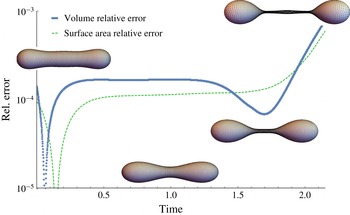
Throughout the simulations, the deviation in the area and volume of the vesicle from their specified values remains within one tenth of a per cent (see figure 2 for a typical example). We also suppress the translation mode in order to cleanly observe pearling transitions.
Conservation of volume and surface area: despite considerable elongation of the vesicle, surface area and volume are conserved to within a tenth of a per cent at all times. Simulation shown here consists of a
 ${\it\nu}=0.6$
vesicle at capillary number
 $\mathit{Ca}=10$
in uniaxial extensional flow. Vesicle snapshots correspond to dimensionless times
 $t=0$
(flow starts),
 $t=1$
,
 $t=1.7$
, and
 $t=2.15$
.

2.3. Comparison with experiments
We compare the stability boundary for pearling to the experiments by Kantsler et al. (Reference Kantsler, Segre and Steinberg2008). The experiments place a tubular vesicle in a cross-slot microfluidic device, measuring the critical extension rate for pearling as a function of the equilibrium aspect ratio of the vesicle
 $L_{0}/(2R_{0})$
, where
 $L_{0}$
and
 $R_{0}$
are the measured length and radius of the vesicle in zero flow. We emphasize that this aspect ratio depends only on the vesicle’s reduced volume
 ${\it\nu}$
, with large values of
 $L_{0}/(2R_{0})$
corresponding to small reduced volumes. Kantsler et al. (Reference Kantsler, Segre and Steinberg2008) normalize the critical extension rate by the time scale
 $t_{\mathit{cap}}=R_{0}^{2}L_{0}{\it\mu}_{\mathit{out}}/{\it\kappa}$
, which yields a critical capillary number
 $\mathit{Ca}_{c}^{\prime }=(4/3){\it\nu}\mathit{Ca}$
(assuming
 $R_{0}=\sqrt{V/({\rm\pi}L_{0})}$
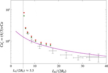
for a nearly cylindrical geometry). In figure 3, we plot the critical capillary number
 $\mathit{Ca}_{c}^{\prime }$
as a function of the equilibrium aspect ratio
 $L_{0}/(2R_{0})$
of the vesicle. The black crosses are experimental data, while the triangles are results from boundary integral simulations. The two sets of triangles reflect the uncertainty in our simulations. The upward-pointing triangles are the highest capillary number where we do not observe pearling, while the downward-pointing triangles are the lowest capillary numbers where we first observe pearling. On the whole, our simulations agree with the experiments quite well. The critical capillary number decreases with increasing equilibrium aspect ratio
 $L_{0}/(2R_{0})$
, with a rapid variation in the range
 $5<L_{0}/(2R_{0})<8$
. Our simulations predict an asymptote in the stability boundary at
 $L_{0}/(2R_{0})\approx 5.5$
(
 ${\it\nu}\approx 0.60$
), which is reasonably close to that found in experiments. The purple dotted curve is a scaling theory based on the critical tension from the idealized pearling model discussed in § 3.2. This theory is only valid for very large equilibrium aspect ratios (
 $L_{0}/(2R_{0})\gg 1$
). The details of this scaling analysis has been published elsewhere and we do not repeat them here (Narsimhan et al.
Reference Narsimhan, Spann and Shaqfeh2014).
Stability boundary: pearling. Critical capillary number
 $\mathit{Ca}_{c}^{\prime }=(4/3){\it\nu}\mathit{Ca}$
versus equilibrium aspect ratio of the vesicle (i.e. aspect ratio at zero flow). Black crosses are from cross-slot microfluidic experiments (Kantsler et al.
Reference Kantsler, Segre and Steinberg2008), while the triangles are from boundary integral simulations (§ 2.2) with the upward- and downward-pointing triangles representing stable and unstable respectively. The purple dashed curve is the scaling theory
 $\mathit{Ca}_{c}^{\prime }=C\ln (L/R)/(L/R)$
for
 $L/R\gg 1$
, with
 $C=6$
.

The experiments exhibit significant scatter in the critical capillary number for three reasons. Most artificially created vesicles are polydisperse and hence exhibit a range of bending moduli, with typical variations on the order of 20 % (Gracia et al.
Reference Gracia, Bezlyepkina, Knorr, Lipowsky and Dimova2010). The vesicles in Kantsler et al. (Reference Kantsler, Segre and Steinberg2008) also exhibit significant thermal fluctuations, which our simulations neglect. Lastly, the measurements may be limited by the optical resolution of the vesicle neck. The typical neck size in the experiments is on the order of
 $1.5{-}2~{\rm\mu}\text{m}$
, which corresponds to a few pixels on the CCD camera. To resolve pearling, the experiments must be able to resolve shape perturbations on the vesicle neck. Since these measurements correspond to very few pixels, there is some uncertainty in determining the exact conditions of pearling.
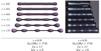
Figure 4 shows snapshots of a vesicle undergoing pearling from our simulations and from experiments. On the whole, our simulations match experiments reasonably well, although our simulations do not capture the dynamics exactly, such as the pearl size, the number of pearls, and the time scale of pearling. One reason for this discrepancy could stem from the uncertainty in the measured capillary number that we mentioned previously. Another reason could be that our simulations neglect the effect of surface viscosity on the vesicle membrane, which becomes significant as the neck size becomes smaller. A typical value of the surface viscosity is
 ${\it\eta}_{s}\sim 5\times 10^{-9}~\text{Pa ms}$
(Dimova et al.
Reference Dimova, Aranda, Bezlyepkina, Nikolov, Riske and Lipowsky2006), which corresponds to a Boussinesq number of
 $Bq\equiv ({\it\eta}_{s}/(R_{\mathit{neck}}{\it\mu}_{\mathit{out}}))\approx 5$
for a
 $1~{\rm\mu}\text{m}$
neck. However, this effect is unlikely to explain the discrepancy, and in fact will make the comparison worse between simulations and experiments, as surface viscosity lowers growth rates for pearls and selects larger pearl sizes (see appendix A). In the next subsection, we show that the pearling phenomenon is sensitive to the initial conditions of the vesicle under flow. We believe that this effect could explain why experiments show smaller pearls and pearl at a somewhat faster time scale than our simulations.
Comparison between simulation and experiment: pearl size and number. Pictures of experiments are from Kantsler (Reference Kantsler2007). The scale bar is
 $10~{\rm\mu}\text{m}$
. All times are scaled by the inverse extension rate
 $\dot{{\it\epsilon}}^{-1}$
.

2.4. Sensitivity to initial conditions
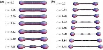
Figure 5 shows a snapshot of two identical vesicles in flow, each seeded with different initial conditions. The first vesicle starts at equilibrium (
 $\mathit{Ca}_{\mathit{init}}=0$
) before turning the flow to the desired capillary number (in this case,
 $\mathit{Ca}_{\mathit{final}}=4$
). The second vesicle starts at steady state at
 $\mathit{Ca}_{\mathit{init}}=1.5$
before increasing the flow to
 $\mathit{Ca}_{\mathit{final}}$
. Both vesicles form pearls, but the second vesicle forms more beads in its central neck. These beads are smaller than in the first vesicle, and the instability occurs more quickly as well. In general, we observe all these trends when a vesicle starts at a larger capillary number, although the phenomenon does not appear to affect the stability boundary for pearling significantly (i.e. figure 3). We suspect the reason behind this phenomenon is as follows: a vesicle that starts in flow will be more elongated and under greater tension than one that starts at equilibrium. The first effect allows the central thread of the vesicle to accommodate more pearls, while the second effect allows the thread to reach the critical tensions required for pearling sooner than the vesicle that starts out at equilibrium. We discuss models for these pearling transitions in § 3.
Role of initial condition in pearling: we show two
 ${\it\nu}=0.49$
vesicles undergoing pearling at
 $\mathit{Ca}_{\mathit{final}}=4$
. The initial shape of vesicle (a) is its shape in zero flow (
 $\mathit{Ca}=0$
). The initial shape of vesicle (b) is its steady-state shape at
 $\mathit{Ca}=1.5$
. The time is scaled by the inverse extension rate
 $\dot{{\it\epsilon}}^{-1}$
. Both vesicles have their critical capillary number between
 $\mathit{Ca}=2.00$
and 2.125.

This phenomenon may explain why the dynamics in our simulations are somewhat different from the ones found experimentally. In our simulations, we often start vesicles at equilibrium (
 $\mathit{Ca}=0$
) before turning on the flow. Pearling instabilities from this procedure usually result in large beads in the central thread. Vesicles in experiments, however, start at finite capillary number as they must be trapped in the cross-slot device before imaging begins. Pearling in this case occurs quickly with multiple, small beads forming in the central neck.
2.5. Relaxation after pearling
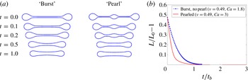
When an elongated droplet relaxes in the absence of flow, the droplet often experiences capillary instabilities in its central thread as it tries to retract back to its equilibrium shape (Bentley & Leal Reference Bentley and Leal1986; Stone Reference Stone1994). None of these instabilities seem to occur for vesicles undergoing relaxation. Figure 6(a) shows two vesicles in flow. The first vesicle is initially unstable, stretching indefinitely in a manner similar to droplets undergoing ‘burst’ (i.e.
 $\mathit{Ca}_{b}<\mathit{Ca}<\mathit{Ca}_{c}$
). The second vesicle is initially undergoing pearling
 $(\mathit{Ca}>\mathit{Ca}_{c})$
. At time
 $t=0$
, the flow halts and both vesicles retract back to their equilibrium shapes. The relaxation process exhibits an exponential decay that can be characterized by a single relaxation time as suggested by Kantsler et al. (Reference Kantsler, Segre and Steinberg2008). It appears that the relaxation depends on the initial configuration of the vesicle, as ‘pearled’ vesicles seem to relax more quickly than non-pearled ones (figure 6
b).
Relaxation of vesicle after flow cessation. (a) Pictures of vesicle relaxing after reaching the ‘burst’ phase and the ‘pearled’ state. The reduced volume is
 ${\it\nu}=0.49$
. The initial capillary numbers are
 $\mathit{Ca}=1.8$
and
 $\mathit{Ca}=3$
for the ‘burst’ and ‘pearled’ states, respectively. (b) Fractional extension of the vesicle versus time for the two vesicles relaxing in (a). The time is non-dimensionalized by the bending time scale
 $t_{b}={\it\mu}_{\mathit{out}}a^{3}/{\it\kappa}$
.

Unlike droplets, we believe that vesicles relax to their equilibrium shape because the vesicle experiences minimal tension in the absence of flow, which eliminates the driving force for capillary instabilities like pearling. Nevertheless, it might still be surprising that the pearled vesicle relaxes to the prolate equilibrium (
 $\mathit{Ca}=0$
) shape, since the pearled shape is far from this local minimum in the free-energy landscape.
3. Idealized models for pearling: infinite cylinder model
3.1. Introduction
When a long vesicle thins continuously in time, its neck becomes nearly cylindrical and its axial stresses vary slowly over length scales comparable to the neck’s radius. We can thus treat the region of pearling as an infinitely long cylinder with constant surface tension
 ${\it\sigma}_{0}$
, where
 ${\it\sigma}_{0}$
is set by the external force (in our case, flow). This quasi-static approximation allows us to determine the vesicle’s stability via equilibrium treatments such as energy minimization, which we pursue in the next subsection. In previous studies, researchers only examined axisymmetric perturbations to the vesicle membrane (Goldstein et al.
Reference Goldstein, Nelson, Powers and Seifert1996; Powers Reference Powers2010; Boedec et al.
Reference Boedec, Jaeger and Leonetti2014; Narsimhan et al.
Reference Narsimhan, Spann and Shaqfeh2014). If we include non-axisymmetric modes, we find that the vesicle can also become unstable under compression via buckling/wrinkling instabilities. This result was first recognized by Foltin (Reference Foltin1994) for tubular vesicles, although it seems to have been overlooked over the years. We examine compressional instabilities for tubular vesicles in § 4.
3.2. Energy minimization
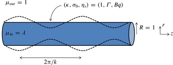
The geometry is shown in figure 7. We have an infinitely long cylinder of radius
 $R$
, bending modulus
 ${\it\kappa}$
, and surface tension
 ${\it\sigma}_{0}$
. We apply a small perturbation to the interface:
 $$\begin{eqnarray}r=R[1+h({\it\phi},z)],\quad |h|\ll 1,\end{eqnarray}$$
and find the conditions under which the cylinder is unstable. We non-dimensionalize all lengths by
 $R$
, all tensions by
 ${\it\kappa}/R^{2}$
, all pressures by
 ${\it\kappa}/R^{3}$
, and all energies by
 ${\it\kappa}$
. Under these assumptions, the Helfrich bending energy of the membrane is
 $$\begin{eqnarray}E=\int 2H^{2}\,\text{d}A+{\it\Gamma}\int \text{d}A-P\int \text{d}V\end{eqnarray}$$
where
 ${\it\Gamma}\equiv {\it\sigma}_{0}R^{2}/{\it\kappa}$
and
 $P\equiv {\rm\Delta}pR^{3}/{\it\kappa}$
are the non-dimensional surface tension and pressure. We expand the energy to second order in the deformation
 $h$
, and find the conditions under which the energy is no longer a local minimum (hence, unstable).

After much algebra and integration by parts, the expression for the bending energy is
 $$\begin{eqnarray}E[h]-E[h=0]=\int \left[-\frac{1}{2}+{\it\Gamma}-P\right]h\,\text{d}{\it\phi}\,\text{d}z+\frac{1}{2}\int h\mathit{\unicode[STIX]{x00A3}}[h]\,\text{d}{\it\phi}\,\text{d}z\end{eqnarray}$$
where the linear operator
 $\mathit{\unicode[STIX]{x00A3}}=(1-P)+[{\rm\nabla}_{s}^{2}+5/2-{\it\Gamma}]{\rm\nabla}_{s}^{2}-2\partial _{z}^{2}$
. The term
 $\boldsymbol{{\rm\nabla}}_{s}\equiv \hat{\boldsymbol{z}}(\partial /\partial z)+\hat{{\bf\phi}}(\partial /\partial {\it\phi})$
is the surface gradient operator of the base-state cylinder (i.e.
 $r=1$
). We expand the deformation into the eigenfunctions of the operator
 $\mathit{\unicode[STIX]{x00A3}}$
, which are Fourier modes:
 $h({\it\phi},z)=\sum _{k}\sum _{n}r_{kn}\exp (\text{i}kz+\text{i}n{\it\phi})$
. Noting that the pressure at mechanical equilibrium satisfies
 $P={\it\Gamma}-1/2$
(i.e. the first variation of the energy (3.3) must vanish), the bending energy (3.3) becomes
 $E[h]-E[0]=(\sum _{k}\sum _{n}|r_{kn}|^{2}L_{kn}({\it\Gamma}))/2$
, where
 $L_{kn}$
is
 $$\begin{eqnarray}L_{kn}({\it\Gamma})={\textstyle \frac{3}{2}}+{\it\Gamma}(k^{2}+n^{2}-1)+2k^{2}+(k^{2}+n^{2})(k^{2}+n^{2}-{\textstyle \frac{5}{2}}).\end{eqnarray}$$
The membrane is unstable when the energy is no longer a local minimum, in other words when
 $L_{kn}<0$
for any
 $k,n>0$
. We summarize the results of the stability analysis below. In short, vesicle stability depends only on the reduced membrane tension
 ${\it\Gamma}={\it\sigma}_{0}R^{2}/{\it\kappa}$
. If this parameter is above a critical value (i.e. the vesicle is under extension), pearling occurs. If this parameter is negative, compressional instabilities like buckling or wrinkling may arise.
-
(a) If the vesicle is under tension (
${\it\Gamma}>0$
):-
(i) the vesicle is unstable to axisymmetric (
$n=0$
) perturbations when
${\it\Gamma}>3/2$
; these modes are pearling modes; -
(ii) all non-axisymmetric modes (
$n>0$
) are stable.
-
-
(b) If the vesicle is under compression (
${\it\Gamma}<0$
):-
(i) the axisymmetric mode (
$n=0$
) is unstable for
${\it\Gamma}<-(3+4\sqrt{2})/2$
; the first non-axisymmetric mode (
$n=1$
) is unstable for
${\it\Gamma}<-3/2$
; all other modes (
$n>1$
) are unstable for
${\it\Gamma}<3/2-n^{2}$
; -
(ii) short-wavelength modes (
$k>1$
) are coined wrinkling transitions, while long-wavelength modes (
$k<1$
) are coined buckling transitions.
-





We plot pictures of the pearling and compressional instabilities in figure 8. The pearling mode (
 $n=0$
) looks qualitatively similar to all previous experiments in pearling (Bar-Ziv & Moses Reference Bar-Ziv and Moses1994; Sinha et al.
Reference Sinha, Gadkari and Thaokar2013). The
 $n=1$
buckling mode looks like a periodic undulation of a line element. The
 $n=2$
buckling mode has an elliptical cross-section that rotates around the axial direction of the cylinder. We do not know which modes are most unstable until we perform a linear stability analysis, taking into account the velocity field induced by the shape perturbation of the membrane. We perform this analysis in appendix A, and state the results here. The growth rate and wavenumber selection of shape perturbations depend on the non-dimensional surface tension
 ${\it\Gamma}$
and
 $$\begin{eqnarray}{\it\lambda}=\frac{{\it\mu}_{\mathit{in}}}{{\it\mu}_{\mathit{out}}},\quad Bq=\frac{{\it\eta}_{s}}{{\it\mu}_{\mathit{out}}R}\end{eqnarray}$$
where
 ${\it\lambda}$
is the viscosity mismatch between the fluid interior and exterior to the vesicle, and
 $Bq$
is the Boussinesq number (ratio of surface viscosity to the bulk viscosity). For typical values of these parameters (
 ${\it\lambda}=1$
,
 $Bq\approx 5$
), the most unstable wavenumber for pearling is
 $kR\approx 0.45$
for
 ${\it\Gamma}\approx 5$
. For compressional instabilities, the axisymmetric wrinkling mode
 $(n=0)$
has its most unstable wavenumber at short wavelength (
 $k<1$
), while the
 $n>1$
modes have their most unstable wavenumbers peaked at
 $k=0$
. In reality, the long-wavelength
 $k=0$
mode is never observed, but is cut off due to the finite length of the vesicle. The
 $n=1$
mode can either be long-wavelength or short-wavelength depending on the tension of the membrane. The most unstable compressional mode is an
 $n=1$
long-wavelength buckling transition for
 $-2.5<{\it\Gamma}<-1.5$
. The
 $n=2$
mode becomes most unstable for
 ${\it\Gamma}$
smaller (
 ${\it\Gamma}<-3$
typically). Although
 $n>1$
modes are peaked at
 $k=0$
, short-wavelength wrinkles also become unstable when the compressional strength is large (
 $|{\it\Gamma}|\gg 1$
).
Modes of instability: (a)
 $n=0$
pearling mode, (b)
 $n=1$
buckling mode, and (c)
 $n=2$
buckling mode. For all three plots, the axial wavenumber is
 $k=0.7$
for illustration purposes.

3.3. Onset of instability: comparison between theory and simulation
In this section, we determine how well the stability criterion offered in § 3.2 performs in terms of predicting the onset of the pearling phenomenon. We examine vesicles with equilibrium aspect ratios
 $L_{0}/(2R_{0})$
between 5.5 and 12.7 (i.e.
 $0.41<{\it\nu}<0.60$
). When we start these vesicles at equilibrium (
 $\mathit{Ca}=0$
) and then increase the flow to above the critical capillary number (
 $\mathit{Ca}>\mathit{Ca}_{c}$
), one pearl forms at the centre of the vesicle, where the tension is at a maximum.
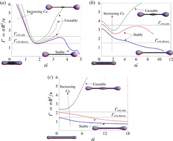
Figure 9 shows the non-dimensional tension at the centre of the vesicle as a function of time, i.e.
 ${\it\Gamma}={\it\sigma}_{\mathit{centre}}R_{\mathit{centre}}^{2}/{\it\kappa}$
. We observe the following trends.
-
(a) At early times, the vesicle’s neck is stretching and becoming more cylindrical. The tension
${\it\Gamma}$
starts large and decreases during this deformation process. -
(b) After this transient period, the tension
${\it\Gamma}$
can increase or decrease depending on its stability to pearling. If the vesicle pearls,
${\it\Gamma}$
increases in time. If the vesicle does not pearl,
${\it\Gamma}$
may increase initially but eventually decreases at long times. The tension for stable vesicles does not exceed a critical value of
${\it\Gamma}_{\mathit{crit}}\approx 2.3$
, 3.5, and 2.1 for
${\it\nu}=0.57$
, 0.49, and 0.41, respectively. These values are larger than the critical value of
${\it\Gamma}_{\mathit{crit}}=1.5$
for the idealized problem of an infinite cylinder (§ 3.2).


This analysis indicates that the idealized problem in § 3.2 under-predicts the critical tension for pearling as long as the vesicle’s aspect ratio is not very large, which in our simulations corresponds to at least
 ${\it\nu}>0.41$
. For these smaller aspect ratio vesicles, we believe that two factors increase the critical tension: the finite length of the cylinder, and the non-uniform tension along the vesicle (see next section).
Tension at centre of vesicle versus time: each curve represents a different value of capillary number. After an initial drop due to vesicle stretching, the tension
 ${\it\Gamma}$
increases if the vesicle pearls (unstable), and eventually decreases if the vesicle is stable. Stable vesicles do not exceed a critical value of
 ${\it\Gamma}$
after this initial transient period, which is larger than the value predicted by theory (
 ${\it\Gamma}=1.5$
). (a) Reduced volume
 ${\it\nu}=0.57$
; the curves represent
 $\mathit{Ca}=3.33$
, 3.5, 3.6, and 4. (b)
 ${\it\nu}=0.49$
;
 $\mathit{Ca}=1.8$
, 2.0, and 2.125. (c)
 ${\it\nu}=0.41$
;
 $\mathit{Ca}=1.25$
, 1.5, and 1.66. We show pictures of stable and unstable vesicles in the insets of each graph. The vesicles in the lower left-hand corner are at equilibrium (
 $\mathit{Ca}=0$
).

3.4. Model to take into account finite length, non-uniform tension
In this section, we develop a model to explain the findings in § 3.3, i.e. that the infinite cylinder model under-predicts the critical surface tension for pearling transitions. We emphasize that this model will not give quantitative results, but rather explains the origin of the discrepancy.
When a vesicle is elongating under flow, we can approximate its shape as a cylinder of length
 $L$
and radius
 $R$
. The shear stresses from the external flow create a tension distribution on the membrane, which is parabolic in the limit of very large aspect ratio (
 $L/R\gg 1$
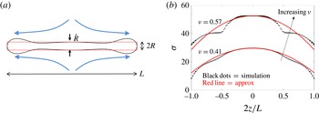
). Figure 10(a) shows a picture of a vesicle as well as its approximating cylinder, just before the vesicle pearls. We see that the cylinder captures the shape of the vesicle in its central neck quite well, but does a poor job at the ends where the vesicle is more dumbbell-shaped. Figure 10(b) shows the tension distribution of the vesicle compared to a parabolic distribution. The parabola does not quantitatively match the tensions, but nevertheless is a better approximation than a constant value, which is the assumption behind the infinite cylinder analysis stated in § 3.2.
Idealized problem: finite length cylinder. (a) Comparison between vesicle and the approximating cylinder just before onset of pearling. The radius
 $R$
is the radius at the centre of the vesicle. The reduced volume is
 ${\it\nu}=0.41$
, and
 $\mathit{Ca}=1.66$
. (b) Tension distribution from simulation and slender body theory just before onset of pearling. The tension is non-dimensionalized by
 ${\it\mu}_{\mathit{out}}\dot{{\it\epsilon}}a$
. Note: slender body theory gives the tension up to an undetermined constant, so we match tensions at the centre of the vesicle. The top curve is
 ${\it\nu}=0.57$
,
 $\mathit{Ca}=3.66$
. The lower curve is
 ${\it\nu}=0.41$
,
 $\mathit{Ca}=1.66$
.

We determine the stability of the approximating cylinder by performing an energy minimization technique akin to the one in § 3.2; the difference now is that we have a finite length cylinder and an external traction due to the pressure and tension fields induced by the flow. In this analysis, we assume that the external traction is frozen, which is not true in actuality as it varies with the configuration of the membrane. Nevertheless, this simplified model reveals additional physics compared to our previous results.
The eigenvalue problem from this energy analysis is
 $$\begin{eqnarray}sh=-{\it\Gamma}(z)\left(h+\frac{\partial ^{2}h}{\partial z^{2}}\right)+\left(\frac{3}{2}h+\frac{1}{2}\frac{\partial ^{2}h}{\partial z^{2}}+\frac{\partial ^{4}h}{\partial z^{4}}\right),\quad -\frac{L}{2R}\leqslant z\leqslant \frac{L}{2R}.\end{eqnarray}$$
This expression is the normal stress balance for the cylinder when its radius is perturbed by a small amount
 $h$
as follows:
 $r=R(1+h),|h|\ll 1$
. The first term on the right-hand side is the perturbation to the capillary pressure with a base-state tension
 ${\it\Gamma}(z)$
. This tension is parabolic as mentioned previously. The second term on the right-hand side is the perturbation to the bending force of the interface. All length scales are non-dimensionalized by the cylinder radius
 $R$
, and the tension
 ${\it\Gamma}(z)$
is non-dimensionalized by the bending modulus exactly as in § 3.2:
 ${\it\Gamma}={\it\sigma}(z)R^{2}/{\it\kappa}$
. The cylinder is unstable when the eigenvalue
 $s$
is negative.
We solve this problem via a spectral-collocation scheme subject to the following constraints:
-
(a) area and volume conservation to
$O(h)$
, i.e. the order of the perturbation; -
(b) fixed centre of mass (to eliminate the translation mode).

Because this problem is a fourth-order ordinary differential equation, we need four boundary conditions to close the eigenvalue problem. We tried several boundary conditions, including combinations of force-free and clamped ends. Here, we show results using clamped ends and natural boundary conditions (
 $h=h^{\prime }=0$
at the ends of the cylinder for the first case, and
 $h^{\prime \prime }=h^{\prime }({\it\Gamma}-1/2)-h^{\prime \prime \prime }=0$
for the second case). As we will see, the stability results do not change qualitatively based on the choice of end conditions. We write the parabolic surface tension
 ${\it\Gamma}(z)$
as
 $$\begin{eqnarray}{\it\Gamma}(z)={\it\Gamma}_{c}-\mathit{Ca}^{\prime \prime }\left(\frac{R}{L}\right)^{2}z^{2},\quad \mathit{Ca}^{\prime \prime }=\frac{{\it\mu}_{\mathit{out}}\dot{{\it\epsilon}}RL^{2}}{{\it\kappa}\ln L/R}\end{eqnarray}$$
where
 ${\it\Gamma}_{c}$
is the tension at the centre of the cylinder, and
 $\mathit{Ca}^{\prime \prime }$
is a capillary number that gives rise to the slowly varying tension on the cylinder. We find that the cylinder becomes unstable if
 ${\it\Gamma}_{c}$
is above a critical value
 ${\it\Gamma}^{\ast }$
. This critical value is a function of the capillary number
 $\mathit{Ca}^{\prime \prime }$
and the slenderness of the cylinder
 ${\it\epsilon}\equiv R/L$
.
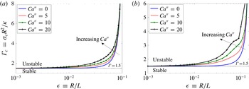
Figure 11 shows that the critical surface tension goes to the value of
 ${\it\Gamma}^{\ast }=1.5$
as the particle slenderness
 ${\it\epsilon}$
goes to zero, which is exactly the result from the infinite cylinder analysis in § 3.2. When the slenderness
 ${\it\epsilon}$
is
 $O(0.1)$
, the critical tension diverges. The values we found for the critical aspect ratios correspond to
 $L/(2R)=1/(2{\it\epsilon})\approx 4.5$
and
 $L/(2R)=1/(2{\it\epsilon})\approx 3.4$
for the case of clamped and natural boundary conditions, respectively. These values compare favourably with the critical value of
 $L/(2R)\approx 5.5$
from our numerical simulations (§ 2.3). We also observe that the critical tension increases as the flow strength (i.e.
 $\mathit{Ca}^{\prime \prime }$
) increases. The physics of these trends can be explained as follows.
-
(a) The most unstable eigenfunctions of (3.6) are long-wavelength modes, which are geometrically disallowed when the particle aspect ratio is small. Thus, finite length effects stabilize the membrane. To destabilize shorter-wavelength modes, the surface tension must increase.
-
(b) Because the surface tension is parabolic, the average tension along the most unstable mode is smaller than the value at the centre of the cylinder. This effect is stabilizing, so non-uniform tension (i.e. increasing
$\mathit{Ca}^{\prime \prime }$
) stabilizes the vesicle.

We emphasize that the model in this section is qualitative, but nevertheless captures physics (finite length effects, parabolic tension) that was neglected in the previous analysis. If we want to quantitatively determine the onset of pearling, we conclude that we have to resort to numerical simulations, as we are unaware of any analytic theory that can accurately resolve the hydrodynamics in this regime.
Stability diagram, finite cylinder: the critical tension at the centre of the cylinder as a function of its aspect ratio (see (3.6) for eigenvalue problem, (3.7) for definition of capillary number). (a) Results for clamped boundary conditions (
 $h=h^{\prime }=0$
at ends). (b) Results for natural boundary conditions (
 $h^{\prime \prime }=({\it\Gamma}-1/2)h^{\prime }-h^{\prime \prime \prime }=0$
at ends). We also plot the critical tension
 ${\it\Gamma}_{c}=1.5$
from the infinite cylinder analysis in § 3.2.

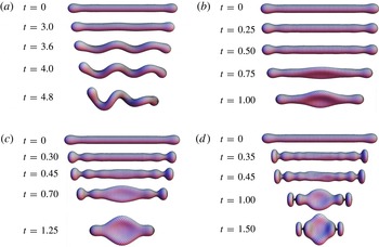
Instabilities in biaxial compressional flow: see (4.1) for definition of flow. All times are non-dimensionalized by the inverse of the compression rate
 $\dot{{\it\epsilon}}^{-1}$
. (a)
 $Ca=0.25$
,
 ${\it\nu}=0.38$
; (b)
 $Ca=1$
,
 ${\it\nu}=0.38$
; (c)
 $Ca=2$
,
 ${\it\nu}=0.38$
; (d)
 $Ca=8$
,
 ${\it\nu}=0.38$
.

4. Wrinkling and buckling instabilities
In the idealized problem in § 3.2, we found that a tubular vesicle may undergo buckling/wrinkling if its surface tension is negative, i.e. the vesicle is under compression. In this section, we verify the existence of these instabilities by performing numerical simulations. Note: the transitions we observe are quite different from the case of quasi-spherical vesicles (Kantsler et al.
Reference Kantsler, Segre and Steinberg2007; Turitsyn & Vergeles Reference Turitsyn and Vergeles2008; Levant et al.
Reference Levant, Abreu, Seifert and Steinberg2014). For example, tubular vesicles undergo wrinkling instabilities at much lower compressional strengths than quasi-spherical ones (
 $\mathit{Ca}\sim O(1)$
versus
 $\mathit{Ca}\sim O(100)$
). Tubular vesicles can also transition to permanent, buckled states, whereas all compressional instabilities for quasi-spherical vesicles are transient as far as we are aware.
Figure 12 shows a snapshot of the buckling instabilities observed for tubular vesicles. We take an equilibrium prolate vesicle (
 $\mathit{Ca}=0$
) and apply a biaxial-compressional flow:
 $$\begin{eqnarray}\boldsymbol{u}^{\infty }=\dot{{\it\epsilon}}[{\textstyle \frac{1}{2}}x,{\textstyle \frac{1}{2}}y,-z]\end{eqnarray}$$
where the
 $z$
direction is the initial orientation of the vesicle, and the stagnation point
 $(0,0,0)$
coincides with the vesicle’s centre of mass. The capillary number
 $\mathit{Ca}\equiv {\it\mu}_{\mathit{out}}\dot{{\it\epsilon}}a^{3}/{\it\kappa}$
gives a measure of the relative strength of compression. A few observations should be noted.
-
(a) At very small capillary numbers (
$\mathit{Ca}\ll 1$
), the vesicle transitions from a prolate shape to an oblate shape. The deformation is axisymmetric and no instability occurs. -
(b) As the capillary number increases, long-wavelength buckling appears (figure 12 a). The vesicle transitions to a sinusoidal filament with a slight helical pitch. These shapes are similar to the long-wavelength
$n=1$
modes discussed in § 3.2 (see figure 8
b). -
(c) At a higher capillary number, the centre of the vesicle breaks symmetry to form a biconcave cross-section (figure 12 b). The cross-section does not exhibit much helicity along the axial coordinate, so the instability is low-wavenumber (
$k\approx 0$
). These shape transitions are similar to the long-wavelength,
$n=2$
modes discussed in § 3.2, which form an elliptical, non-rotating cross-section. -
(d) More complex shapes arise at even higher capillary numbers (figure 12 c,d). At first, the lobes at the vesicle ends pinch and propagate axisymmetric wrinkles towards the centre. These wrinkles disappear when the dominant biconcave shape manifests itself, as mentioned in point (c). Sometimes (figure 12 d), higher-order transient wrinkles appear at the centre as well. These wrinkles are similar to the short-wavelength
$n=2$
modes (figure 8
c), which are characterized by ellipsoidal cross-sections that rotate around the axial coordinate. The highest capillary number we observe exhibits near pinch-off (pearling) at the ends of the vesicle as well.


These trends are consistent with the predictions from the idealized problem: the linear stability of an infinitely long cylinder under constant compression (appendix A). In this analysis, the
 $n=1$
buckling mode first becomes unstable for a narrow range of compressional strengths, and then the
 $n=2$
mode dominates as the compressional strength increases (figure 16
a). The
 $n=2$
modes are most unstable at zero wavenumber (figure 15
a), which explains why we observe negligible helicity for the final vesicle shapes in our simulations in figure 12(b–d). At large compressional strengths, sub-dominant, short-wavelength modes start becoming unstable, especially
 $n=0$
and
 $n=2$
modes as indicated in figure 15(b). This result could explain why axisymmetric and elliptical wrinkles arise at high capillary number (figure 12
c,d). Note: the linear stability analysis cannot explain all observed phenomena, such as wrinkles propagating from the end of the vesicle towards the centre (figure 12
c,d). In fact, the stability analysis predicts only standing waves, which is clearly a shortcoming. Nevertheless, it is remarkable that this simple theory can qualitatively explain many of the observations in our simulations. To understand the origin of the wave propagation phenomenon, we suggest developing a model similar to the sudden axial compression of a thin-walled cylinder found in the solid mechanics literature (Lindberg & Florence Reference Lindberg and Florence1987). In this situation, an axisymmetric wave propagates towards the centre of the cylinder if the radius at the ends is slightly larger than the rest of the body. These waves are transient, and the most unstable mode for static deformation dominates the long-time behaviour. It appears that this idea captures the basic elements of our simulated observations, although we will examine the details in a future work.
In microfluidic experiments, the biaxial flow in (4.1) is rarely realized. Instead, the velocity field observed in a cross-slot device is a planar compressional flow:
 $$\begin{eqnarray}\boldsymbol{u}^{\infty }=\dot{{\it\epsilon}}[x,0,-z].\end{eqnarray}$$
As before, the
 $z$
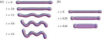
-axis corresponds to the initial orientation of the vesicle. We perform the same simulations as in figure 12 but now in planar compressional flow. In general, we observe the same qualitative trends as above, i.e. long-wavelength buckling at small capillary numbers (figure 13
a) and biconcave cross-sections at higher capillary numbers (figure 13
b). In the biaxial flow case, the orientation of the biconcave cross-section is arbitrary: it is determined by small perturbations in the initial condition set by numerical noise. In the planar compression case, however, the orientation is set by the flow, i.e. the axis of extension (
 $x$
-direction). Another notable difference is that we do not observe transient wrinkling in the case of planar compressional flow. Again, the theories discussed in appendix A elucidate the basic physics of these shape transitions. However, we do not expect these theories to be quantitative as they neglect a host of effects such as the vesicle’s finite length and its non-uniform tension on the interface.
Instabilities in planar compressional flow: see (4.2) for definition of flow. All times are non-dimensionalized by the inverse of the compression rate
 $\dot{{\it\epsilon}}^{-1}$
. (a)
 $Ca=0.25$
,
 ${\it\nu}=0.38$
; (b)
 $Ca=8$
,
 ${\it\nu}=0.38$
.

The results discussed here are preliminary. For example, we do not explore the full parameter space in capillary number and reduced volume, which would yield a set of stability diagrams for the shape transitions discussed above. We also do not discuss how the viscosity contrast between the inner and outer fluid modifies these instabilities. If the stability analysis in appendix A is applicable, we suspect that this parameter will not modify the stability of the vesicles in compressional flows, but will affect the time scale of the instability and the wavenumber selection. Lastly, we do not discuss what role the vesicle’s initial orientation plays in its shape dynamics. In all experiments, the vesicle is never oriented exactly along the axis of compression, and thus rotates towards the extension axis and stretches. The compressional instabilities discussed above can thus arise only if the time scale of their formation is much smaller than the time scale of rotation. In the future, we would like to characterize what initial orientations yield buckling, which would provide useful information as to whether these transitions could be observed experimentally. We suspect that compressional instabilities will be difficult to observe in flow but could be easier to visualize under uniaxial compression via optical tweezers (Chen Reference Chen2012). The analysis of the idealized problem in appendix A suggests that any type of compression can initiate buckling, which is an interesting claim that must be verified via further theory and experiments. Clearly, this area is ripe for future study.
5. Conclusions and future directions
In § 2, we describe boundary integral simulations to examine the pearling of vesicles under elongational flows. Our simulations neglect thermal fluctuations and membrane viscosity, but nevertheless capture the stability criterion for pearling quite well, agreeing with the latest experiments by Kantsler et al. (Reference Kantsler, Segre and Steinberg2008). We also find that the initial configuration of the vesicle in flow plays a big role in determining the size and number of pearls in the central neck. In general, vesicles that start in a more elongated state form a larger number of pearls. The size of the pearls and the time scale of pearling are both reduced as well. Lastly, we discuss the relaxational dynamics of a pearled vesicle after flow cessation. Unlike droplets, vesicles relax to their equilibrium shape after flow stops. This result can be explained by noting that a vesicle’s tension decreases in the absence of flow, which in turn reduces the driving force for capillary pinch-off events.
In the second part of the paper (§ 3), we examine an idealized model for vesicle pearling: an infinitely long cylinder with a constant tension and bending modulus. This problem has been explored previously (Goldstein et al.
Reference Goldstein, Nelson, Powers and Seifert1996; Powers Reference Powers2010; Boedec et al.
Reference Boedec, Jaeger and Leonetti2014), but we perform the most comprehensive linear stability analysis in appendix A, including the effects of surface viscosity and non-axisymmetric modes, while also including the effects of tangential stresses on the dispersion relationship (which earlier authors neglected (Goldstein et al.
Reference Goldstein, Nelson, Powers and Seifert1996; Powers Reference Powers2010)). We find that this model captures the critical tension for instability when the reduced volume is very low (
 ${\it\nu}\ll 1$
), but under-predicts the critical tension for
 ${\it\nu}>0.41$
. We offer reasons for the discrepancy in § 3.4. In short, finite length effects and non-uniform tension from flow significantly increase the critical tension.
The idealized problem in the previous paragraph predicts that tubular vesicles exhibit additional shape instabilities if they are under compression. We verify these predictions by performing large-scale numerical simulations of vesicles in compressional flow (§ 4). Unlike quasi-spherical vesicles (Kantsler et al.
Reference Kantsler, Segre and Steinberg2007; Levant et al.
Reference Levant, Abreu, Seifert and Steinberg2014), these instabilities occur at low compressional strengths (
 $\mathit{Ca}\sim O(1)$
), and can lead to the formation of permanent, buckled states (figures 12 and 13). We have not fully quantified the stability boundaries for these buckled states in terms of the vesicle’s reduced volume
 ${\it\nu}$
and capillary number
 $\mathit{Ca}$
. These studies will be continued in the future.
Acknowledgements
The authors acknowledge support from the US Army High Performance Computing Research Center (AHPCRC), and support from Stanford University’s Certainty computer cluster that is funded by the American Recovery and Reinvestment Act (ARRA) of 2009 (grant no. W911NF07200271). The authors would also like to acknowledge NSF funding under CBET 1066263. V.N. is funded through the generous support of the Stanford Lieberman Fellowship.
Appendix A. Linear stability analysis for pearling/buckling of an infinitely long cylinder
A.1. Problem setup
We have an infinitely long, cylindrical vesicle of radius
 $R$
, surface tension
 ${\it\sigma}_{0}$
, bending modulus
 ${\it\kappa}$
, and surface viscosity
 ${\it\eta}_{s}$
. The fluid outside the vesicle has viscosity
 ${\it\mu}$
, while the fluid inside the vesicle has viscosity
 ${\it\lambda}{\it\mu}$
. If we apply a small perturbation
 $r=R[1+h(z,{\it\phi},t)]$
to the interface, where
 $\Vert h\Vert \ll 1$
, under what conditions will the membrane become unstable (i.e.
 $(1/h)(\text{d}h/\text{d}t)>0$
)? This linear stability analysis is similar to the classic Rayleigh–Plateau problem of the breakup of a liquid cylindrical jet (Tomotika Reference Tomotika1935). In particular, the extension to vesicles was studied first by Bar-Ziv & Moses (Reference Bar-Ziv and Moses1994) and then by Goldstein et al. (Reference Goldstein, Nelson, Powers and Seifert1996), Gurin, Lebedev & Muratov (Reference Gurin, Lebedev and Muratov1996), Powers (Reference Powers2010), Boedec et al. (Reference Boedec, Jaeger and Leonetti2014), and Narsimhan et al. (Reference Narsimhan, Spann and Shaqfeh2014). In the first four papers, the authors obtain the correct stability criterion for pearling, but obtain incorrect growth rates and wavenumber selection, as they neglect the tangential stress balance in their derivations. The latest two papers correct these mistakes (Boedec et al.
Reference Boedec, Jaeger and Leonetti2014; Narsimhan et al.
Reference Narsimhan, Spann and Shaqfeh2014), but do not examine the effects of membrane surface viscosity (
 ${\it\eta}_{s}$
) or non-axisymmetric perturbations. In this section, we provide the most general, unifying treatment of this problem, taking into account both of these effects. We borrow heavily from previous works, as Gurin et al. (Reference Gurin, Lebedev and Muratov1996) treats non-axisymmetric modes, while Powers (Reference Powers2010) provides the framework to add surface viscosity.
We provide a picture of the geometry in figure 7. The coordinate system is cylindrical coordinates
 $(r,{\it\phi},z)$
, and the deformation of the membrane is broken into Fourier modes:
 $$\begin{eqnarray}h(z,{\it\phi},t)={\it\epsilon}\mathop{\sum }_{k,n}r_{kn}(t)\exp (\text{i}kz+\text{i}n{\it\phi})\end{eqnarray}$$
where
 ${\it\epsilon}$
is a small number (
 ${\it\epsilon}\ll 1$
), and
 $k$
and
 $n$
are wavenumbers in the axial and azimuthal directions. Our goal is to find a dispersion relationship for each mode
 $r_{kn}$
by solving the Stokes flow around the cylinder (i.e.
 ${\it\eta}{\rm\nabla}^{2}\boldsymbol{u}=\boldsymbol{{\rm\nabla}}p$
and
 $\boldsymbol{{\rm\nabla}}\boldsymbol{\cdot }\boldsymbol{u}=0$
, where
 ${\it\eta}$
is the viscosity of the medium).
From here on, we write quantities in non-dimensional form unless otherwise specified. All lengths are scaled by the cylinder radius
 $R$
, all times by the bending time scale
 $t_{b}={\it\mu}R^{3}/{\it\kappa}$
, and all velocities by
 $U=R/t_{b}={\it\kappa}/({\it\mu}R^{2})$
. We scale all stresses and pressures by
 ${\it\mu}U/R={\it\kappa}/R^{3}$
, and all surface tensions by
 ${\it\kappa}/R^{2}$
. This process yields three parameters that completely describe the dynamics of the vesicle:
 $$\begin{eqnarray}{\it\lambda}=\frac{{\it\mu}_{\mathit{in}}}{{\it\mu}_{\mathit{out}}},\quad {\it\Gamma}=\frac{{\it\sigma}_{0}R^{2}}{{\it\kappa}},\quad Bq=\frac{{\it\eta}_{s}}{R{\it\mu}}.\end{eqnarray}$$
The first term
 ${\it\lambda}$
is the viscosity ratio between the fluid inside the vesicle to that outside the vesicle. The second term
 ${\it\Gamma}$
is the initial surface tension of the vesicle normalized by the bending forces. The last term
 $Bq$
is the Boussinesq number, which is the ratio of interfacial viscous forces to bulk viscous forces. For most systems, all three parameters are
 $O(1)$
(see Dimova et al. (Reference Dimova, Aranda, Bezlyepkina, Nikolov, Riske and Lipowsky2006) for estimates of surface viscosity). In this appendix, we examine all values of these parameters.
We solve the Stokes flow subject to the boundary conditions: (a) continuity of velocity,
 $[[\boldsymbol{u}]]=0$
; (b) surface incompressibility,
 $\boldsymbol{{\rm\nabla}}_{s}\boldsymbol{\cdot }\boldsymbol{u}=0$
; (c) kinematic boundary condition,
 $\partial r/\partial t+\boldsymbol{u}\boldsymbol{\cdot }\boldsymbol{{\rm\nabla}}r=0$
; and (d) membrane force balance,
 $[[{\bf\tau}\boldsymbol{\cdot }\boldsymbol{n}]]=\boldsymbol{f}^{{\it\sigma}}+\boldsymbol{f}^{\mathit{bend}}+\boldsymbol{f}^{s-v}$
. In these expressions,
 $[[\cdots ]]$
represents the jump of a quantity across the interface (outside minus inside). The viscous stresses are
 ${\bf\tau}={\it\eta}(\boldsymbol{{\rm\nabla}}\boldsymbol{u}+(\boldsymbol{{\rm\nabla}}\boldsymbol{u})^{\text{T}})-p\boldsymbol{I}$
, and the membrane tractions
 $\boldsymbol{f}^{{\it\sigma}}$
,
 $\boldsymbol{f}^{\mathit{bend}}$
, and
 $\boldsymbol{f}^{s-v}$
are resistances of the vesicle’s phospholipid bilayer to surface tension, bending, and surface viscosity. We note that surface tension is a spatially varying field that enforces surface incompressibility (i.e. condition (b)). We write the expressions for the membrane tractions as (see Zhong-Can & Helfrich Reference Zhong-Can and Helfrich1989 for bending and Scriven Reference Scriven1960 for surface viscosity)
 $$\begin{eqnarray}\left.\begin{array}{@{}c@{}}\boldsymbol{f}^{{\it\sigma}}=2H{\it\sigma}\boldsymbol{n}-\boldsymbol{{\rm\nabla}}_{s}{\it\sigma}\\ \boldsymbol{f}^{\mathit{bend}}=(4KH-4H^{3}-2{\rm\nabla}_{s}^{2}H)\boldsymbol{n}\\ \boldsymbol{f}^{s-v}=Bq\boldsymbol{{\rm\nabla}}_{s}\boldsymbol{\cdot }\{\boldsymbol{P}(\boldsymbol{{\rm\nabla}}_{s}\boldsymbol{\cdot }\boldsymbol{u})-\boldsymbol{P}\boldsymbol{\cdot }[(\boldsymbol{{\rm\nabla}}_{s}\boldsymbol{u})+(\boldsymbol{{\rm\nabla}}_{s}\boldsymbol{u})^{\text{T}}]\boldsymbol{\cdot }\boldsymbol{P}\}.\end{array}\right\}\end{eqnarray}$$
For these expressions, we define the surface projection operator as
 $\boldsymbol{P}=\boldsymbol{I}-\boldsymbol{n}\boldsymbol{n}$
and the surface gradient as
 $\boldsymbol{{\rm\nabla}}_{s}=\boldsymbol{P}\boldsymbol{\cdot }\boldsymbol{{\rm\nabla}}$
, where
 $\boldsymbol{n}$
is the outward-pointing normal vector. We define the mean and Gaussian curvatures as
 $H$
and
 $K$
, where the sign convention chosen is such that
 $H$
is positive for a cylinder.
In the next section (§ A.2), we perform a perturbation expansion of the normal stress balance in terms of
 ${\it\epsilon}$
, the membrane deformation (see (A 1)). We solve for the fluid velocity in § A.3, and find dispersion relation for each Fourier mode. In § A.4, we discuss the results.
A.2. Perturbation expansion of normal stress balance
We expand all quantities as follows:
 $f=f_{0}+{\it\epsilon}f_{kn}\exp (\text{i}kn+\text{i}n{\it\phi})$
, where
 $f_{0}$
are quantities for the vesicle at rest, while
 $f_{kn}$
are quantities that are linear in the deformation of the membrane (i.e. Fourier modes
 $r_{kn}$
). As an example, we write out the expansion for the cylinder radius, as well as the pressure, surface tension, and velocity fields:
 $$\begin{eqnarray}\left.\begin{array}{@{}c@{}}r=1+{\it\epsilon}r_{kn}\exp (\text{i}kz+\text{i}n{\it\phi})\\ p=p_{0}+{\it\epsilon}p_{kn}\exp (\text{i}kz+\text{i}n{\it\phi})\\ {\it\sigma}={\it\Gamma}+{\it\epsilon}{\it\sigma}_{kn}\exp (\text{i}kz+\text{i}n{\it\phi})\\ \boldsymbol{u}={\it\epsilon}\boldsymbol{u}_{kn}\exp (\text{i}kz+\text{i}n{\it\phi}).\end{array}\right\}\end{eqnarray}$$
We expand the normal stress balance to
 $O({\it\epsilon})$
around the cylinder
 $r=1$
, obtaining
 $$\begin{eqnarray}-[[p_{kn}]]-{\it\sigma}_{kn}-\hat{\boldsymbol{r}}\boldsymbol{\cdot }\boldsymbol{f}_{kn}^{s-v}=2H_{kn}{\it\Gamma}+f_{kn}^{\mathit{bend}}.\end{eqnarray}$$
To evaluate the perturbation curvature
 $H_{kn}$
and bending forces
 $f_{kn}^{\mathit{bend}}$
to
 $O({\it\epsilon})$
, we first determine the principal curvatures of the interface to
 $O({\it\epsilon})$
:
 $$\begin{eqnarray}C_{1}=1+{\it\epsilon}(n^{2}-1)r_{kn}\exp (\text{i}kz+\text{i}n{\it\phi}),\quad C_{2}={\it\epsilon}k^{2}r_{kn}\exp (\text{i}kz+\text{i}n{\it\phi}).\end{eqnarray}$$
The mean and Gaussian curvatures are
 $H=0.5(C_{1}+C_{2})$
and
 $K=C_{1}C_{2}$
. Similarly, the surface Laplacian of
 $H$
is
 ${\rm\nabla}_{s}^{2}H=(\partial _{z}^{2}+\partial _{{\it\phi}}^{2})H$
. Thus, examining (A 5), the normal stresses simplify to
 $$\begin{eqnarray}\displaystyle & \displaystyle -[[p_{kn}]]-{\it\sigma}_{kn}-\hat{\boldsymbol{r}}\boldsymbol{\cdot }\boldsymbol{f}_{kn}^{s-v}=L_{kn}({\it\Gamma})r_{kn} & \displaystyle\end{eqnarray}$$
 $$\begin{eqnarray}\displaystyle & \displaystyle L_{kn}({\it\Gamma})={\it\Gamma}(k^{2}+n^{2}-1)+3/2+2k^{2}+(k^{2}+n^{2})(k^{2}+n^{2}-5/2). & \displaystyle\end{eqnarray}$$
The right-hand side of (A 7) is the normal stress contribution due to perturbations in the mean curvature and bending forces. The left-hand side are contributions from the perturbation flow, which consists of pressure, Marangoni, and surface viscosity contributions. The left-hand side is linearly dependent on deformation rate of the interface
 $(\text{d}/\text{d}t)(r_{kn})$
, and thus we write it as
 ${\it\Lambda}_{kn}{\dot{r}}_{kn}$
, where
 ${\it\Lambda}_{kn}$
is a function of the viscosity ratio
 ${\it\lambda}$
and Boussinesq number
 $Bq$
. In the next section, we compute
 ${\it\Lambda}_{kn}$
by solving the Stokes flow around a cylindrical vesicle. When we determine this quantity, we obtain the dispersion relation for each Fourier mode, and hence complete our analysis.
A.3. Solving Stokes equations (determine
${\it\Lambda}_{kn}$
)

The Stokes velocity and pressure fields for each Fourier mode in a cylindrical geometry can be expressed as (see Happel & Brenner Reference Happel and Brenner1973)
 $$\begin{eqnarray}\displaystyle & \displaystyle \boldsymbol{u}_{kn}\exp (\text{i}kz+\text{i}n{\it\phi})=\boldsymbol{{\rm\nabla}}{\it\psi}+\boldsymbol{{\rm\nabla}}\wedge ({\it\Omega}\hat{\boldsymbol{z}})+r\frac{\partial }{\partial r}(\boldsymbol{{\rm\nabla}}{\it\Pi})+\hat{\boldsymbol{z}}\frac{\partial {\it\Pi}}{\partial z} & \displaystyle\end{eqnarray}$$
 $$\begin{eqnarray}\displaystyle & \displaystyle p_{kn}\exp (\text{i}kz+\text{i}n{\it\phi})=-2\tilde{{\it\eta}}\frac{\partial ^{2}{\it\Pi}}{\partial z^{2}} & \displaystyle\end{eqnarray}$$
 ${\it\psi}$
,
 ${\it\Omega}$
, and
 ${\it\Pi}$
are scalar harmonic functions written as follows:
 $$\begin{eqnarray}\{{\it\psi},{\it\Omega},{\it\Pi}\}=\{A_{kn},\text{i}B_{kn},C_{kn}\}\unicode[STIX]{x1D60E}_{n}(kr)\exp (\text{i}kz+\text{i}n{\it\phi}).\end{eqnarray}$$
In the equations above,
 $\tilde{{\it\eta}}$
is the non-dimensional viscosity of the medium, which is one outside the vesicle and
 ${\it\lambda}$
inside the vesicle. The functions
 $\unicode[STIX]{x1D60E}_{n}(kr)$
are modified Bessel functions, being
 $I_{n}(kr)$
inside the vesicle and
 $\text{e}^{\text{i}{\rm\pi}n}K_{n}(kr)$
outside the vesicle. We write
 $\unicode[STIX]{x1D60E}_{n}(kr)$
in this fashion so that the derivative formulae for Bessel functions are the same in all regions of space (for example,
 $\unicode[STIX]{x1D60E}_{n}^{\prime }(x)=0.5[\unicode[STIX]{x1D60E}_{n-1}(x)+\unicode[STIX]{x1D60E}_{n+1}(x)]$
). To solve for the velocity and pressure, we determine the six coefficients
 $\{A_{kn},B_{kn},C_{kn}\}$
inside and outside the vesicle using the boundary conditions of the flow.
The velocity and tangential stress boundary conditions, transferred onto the cylinder’s surface
 $r=1$
are
-
(a) continuity of velocity:
$[[u_{kn}^{{\it\phi}}]]=0$
,
$[[u_{kn}^{z}]]=0$
; -
(b) kinematic:
$u_{kn}^{r}={\dot{r}}_{kn}$
for inner and outer flow; -
(c) surface incompressibility:
$\text{i}ku_{kn}^{z}+\text{i}nu_{kn}^{{\it\phi}}+u_{kn}^{r}=0$
for outer flow; -
(d) tangential stress:
$[[{\it\tau}_{kn}^{rz}]]+\text{i}k{\it\sigma}_{kn}-\hat{\boldsymbol{z}}\boldsymbol{\cdot }\boldsymbol{f}_{kn}^{s-v}=0$
,
$[[{\it\tau}_{kn}^{r{\it\phi}}]]+\text{i}n{\it\sigma}_{kn}-\hat{{\bf\phi}}\boldsymbol{\cdot }\boldsymbol{f}_{kn}^{s-v}=0$
.





These conditions provide seven equations for the coefficients
 $\{A_{kn},B_{kn},C_{kn}\}$
inside and outside the vesicle, as well as the surface tension
 ${\it\sigma}_{kn}$
on the membrane. We solve these unknowns in terms of the interfacial deformation rate
 ${\dot{r}}_{kn}$
, and then evaluate the flow contribution to the normal stress balance (i.e. the left-hand side of (A 7)):
 $$\begin{eqnarray}-[[p_{kn}]]-{\it\sigma}_{kn}-\hat{\boldsymbol{r}}\boldsymbol{\cdot }\boldsymbol{f}_{kn}^{s-v}={\it\Lambda}_{kn}({\it\lambda},Bq){\dot{r}}_{kn}.\end{eqnarray}$$
The term
 ${\it\Lambda}_{kn}{\dot{r}}_{kn}$
balances
 $L_{kn}r_{kn}$
, which is the normal stress due to perturbations in curvature and bending (A 7). We thus have a dispersion relationship for each Fourier mode. If we define the growth rate of each mode as
 $s={\dot{r}}_{kn}(t)/r_{kn}(t)$
, the growth rate is
 $$\begin{eqnarray}s=\frac{L_{kn}({\it\Gamma})}{{\it\Lambda}_{kn}({\it\lambda},Bq)}.\end{eqnarray}$$
This equation is the central result of this stability analysis. We compute the growth rates in § A.4, and determine the conditions under which the vesicle becomes unstable (
 $s>0$
). We also determine what wavenumbers
 $k$
and
 $n$
dominate during instability.
Note: algebraic details for the computation of
 ${\it\Lambda}_{kn}$
are provided in Narsimhan (Reference Narsimhan2014, pp. 172–175).
A.4. Results
The growth rate of each Fourier mode
 $(k,n)$
is a ratio of two factors:
 $s=L_{kn}/{\it\Lambda}_{kn}$
, where
 $L_{kn}$
is given by (A 7), (A 8), and
 ${\it\Lambda}_{kn}$
is given by (A 12). Physically,
 $L_{kn}$
is the contribution to the normal stresses from perturbations of the bending force and mean curvature.
 ${\it\Lambda}_{kn}$
is the contribution due to hydrodynamics.
 ${\it\Lambda}_{kn}$
is always negative, so instability occurs only when
 $L_{kn}<0$
. We previously discussed the conditions for instability in § 3.2. Here, we discuss how the hydrodynamics affect wavenumber selection as well as the time scale of pearling.
A.4.1. Plots and wavenumber selection
Pearling modes
In § 3.2, we show that a cylindrical vesicle is always stable to non-axisymmetric perturbations (
 $n>0$
) when its initial surface tension is positive (
 ${\it\Gamma}>0$
). We thus only examine the
 $n=0$
modes for the pearling transitions. In this case, the growth rate has an explicit expression:
 $$\begin{eqnarray}\left.\begin{array}{@{}c@{}}s(k,n=0)=L_{k0}/{\it\Lambda}_{k0}\quad L_{k0}=(k^{2}-1){\it\Gamma}+{\textstyle \frac{3}{2}}-{\textstyle \frac{1}{2}}k^{2}+k^{4}\\ {\it\Lambda}_{k0}=2(k^{2}+1)[{\it\beta}^{-1}K_{1}^{2}-{\it\lambda}{\it\alpha}^{-1}I_{1}^{2}]-4Bq\\ {\it\alpha}=I_{1}^{2}k^{2}-I_{0}^{2}k^{2}+2I_{0}I_{1}k\quad {\it\beta}=K_{1}^{2}k^{2}-K_{0}^{2}k^{2}-2K_{0}K_{1}k.\end{array}\right\}\end{eqnarray}$$
For the above, all modified Bessel functions
 $I$
and
 $K$
are evaluated at the wavenumber
 $k$
. When the vesicle has zero surface viscosity (
 $Bq=0$
), we recover the results of Boedec et al. (Reference Boedec, Jaeger and Leonetti2014) and Narsimhan et al. (Reference Narsimhan, Spann and Shaqfeh2014). We note that Powers (Reference Powers2010) under-predicts the surface viscosity contribution to
 ${\it\Lambda}_{k0}$
by a factor of one-half. The reason for this discrepancy is that the author neglects the interfacial tangential stress balance in his derivation, which leads to an under-prediction for the dissipation on the interface.
In a previous paper, we discussed extensively how the viscosity ratio
 ${\it\lambda}$
affects the growth rate and wavenumber selection for the pearling instability (see Narsimhan et al.
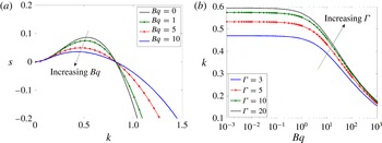
Reference Narsimhan, Spann and Shaqfeh2014, especially figures 21 and 22). Here, we discuss the effect that surface viscosity has on the dynamics. Figure 14 shows that increasing
 $Bq$
decreases the growth rate of pearling and shifts the most unstable wavenumber to lower values (which indicate larger pearls). Surface viscosity only has an appreciable effect when
 $Bq\sim O(1)$
or larger.
Effect of surface viscosity on pearling. (a) Growth rate
 $s$
of the axisymmetric (
 $n=0$
) mode versus wavenumber
 $k$
as a function of Boussinesq number
 $Bq$
. In this plot,
 ${\it\Gamma}=5$
, and
 ${\it\lambda}=1$
. (b) Most unstable wavenumber as a function of
 $Bq$
. In this plot,
 ${\it\lambda}=1$
. The growth rate is scaled by the inverse of the bending time
 $t_{b}^{-1}={\it\kappa}/({\it\mu}R^{3})$
, while the wavenumber is scaled by the inverse of the cylinder radius
 $R^{-1}$
.

Buckling and wrinkling
For axisymmetric deformations (
 $n=0$
), the growth rate of the shape perturbations satisfies the same expressions as (A 14). The expressions for non-axisymmetric deformations (
 $n>0$
) are much more complicated, so we do not write them, but rather explain the trends in the graphs below.
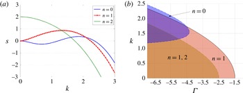
Figure 15(a) shows a typical curve of growth rate
 $s$
versus perturbation wavenumber
 $k$
for three different azimuthal modes (
 $n=0$
, 1, and 2). The axisymmetric mode (
 $n=0$
) is unstable for a small band of short-wavelength deformations (
 $k>1$
), while all
 $n>1$
modes are most unstable at infinite wavelength (
 $k=0$
). The range of unstable wavenumbers depends only on the non-dimensional surface tension
 ${\it\Gamma}$
. As the vesicle becomes more strongly compressed (i.e.
 $|{\it\Gamma}|$
becomes larger), it becomes unstable to a wider range of wavenumbers (figure 15
b). The non-axisymmetric modes (
 $n>0$
) contain long-wavelength deformations (
 $k<1$
) at low compressional strengths (
 $|{\it\Gamma}|<2.5$
), but incorporate short-wavelength deformations (
 $k>1$
) as compression becomes stronger. The axisymmetric mode (
 $n=0$
) remains short-wavelength (
 $k>1$
) at all tensions.
Growth rates and range of unstable wavenumbers, compressional instabilities. (a) Growth rate
 $s$
versus the axial wavenumber
 $k$
for azimuthal modes
 $n=0$
, 1, and 2. The surface tension is
 ${\it\Gamma}=-6.5$
, the viscosity ratio is
 ${\it\lambda}=1$
, and the Boussinesq number is
 $Bq=0$
. We scale growth rates by the inverse of the bending time
 $t_{b}^{-1}={\it\kappa}/({\it\mu}R^{3})$
and wavenumbers by the inverse of the cylinder radius
 $R^{-1}$
. (b) Unstable wavenumbers versus surface tension
 ${\it\Gamma}$
. We examine modes
 $n=0$
, 1, and 2. Shaded regions are unstable.

Maximum growth rate and most unstable wavenumber, compressional instabilities. (a) Maximum growth rate
 $s$
versus surface tension
 ${\it\Gamma}$
for azimuthal modes
 $n=0$
, 1, and 2. For each mode, we plot curves at
 $Bq=0$
, 5, and 10 to indicate how
 $s$
varies with the surface viscosity. The curves are indistinguishable for the
 $n=2$
mode. (b) Most unstable wavenumber
 $k^{\ast }$
versus
 ${\it\Gamma}$
for azimuthal modes
 $n=0$
and
 $n=1$
. For each mode, we plot curves at
 $Bq=0$
, 5, and 10 to indicate how
 $k^{\ast }$
varies with surface viscosity. For all plots, we scale the growth rate by the inverse of the bending time
 $t_{b}^{-1}={\it\kappa}/({\it\mu}R^{3})$
and the wavenumber by the inverse of the cylinder radius
 $R^{-1}$
. The viscosity ratio is
 ${\it\lambda}=1$
.

Figure 16(a) plots the maximum growth rate as a function of surface tension
 ${\it\Gamma}$
for the azimuthal modes
 $n=0$
, 1, and 2. For each mode, we plot curves at
 $Bq=0$
, 5, and 10 to understand the effect of surface viscosity as well. We find that the
 $n=1$
mode appears to be the most unstable for surface tensions between
 $-2.5<{\it\Gamma}<-1.5$
. Slightly below
 ${\it\Gamma}\approx -2.5$
, the
 $n=2$
mode becomes most unstable. As the surface viscosity increases, the vesicle membrane experiences greater dissipation, and hence lower growth rates. We see that this effect is significant for the
 $n=0$
and
 $n=1$
modes, but surprisingly negligible for the
 $n=2$
modes. In fact, we find that all higher-order modes
 $n>1$
are relatively insensitive to surface viscous effects. This analysis suggests that, at least for vesicles, surface viscosity may not be important for describing the physics of highly non-axisymmetric, compressional deformations.
Figure 16(b) plots the most unstable axial wavenumber
 $k$
as a function of surface tension
 ${\it\Gamma}$
and Boussinesq number
 $Bq$
. The most important point to take away is that
 $k$
follows the same trends as in the pearling case. The most unstable wavenumber increases as
 $|{\it\Gamma}|$
increases, but decreases as
 $Bq$
increases. It appears that surface viscosity does not have a large effect on wavenumber selection for the axisymmetric
 $(n=0)$
modes, while it has a big effect for the
 $n=1$
modes. Note: for higher-order modes (
 $n>1$
), the most unstable wavenumber is always
 $k=0$
, so we do not plot the results here.