


1 Introduction
A subfactor N is a unital subalgebra of a type
 $II_1$
-factor M, which is itself a
 $II_1$
factor, that satisfies
 $1_N=1_M$
. An important invariant of a subfactor is the Jones index
 $[M:N]$
[Reference Jones11], which generalizes the subgroup index. The Jones index measures how much ‘bigger’ M is compared with N. In view of the fact that the subfactor theory deals with the relative position of a subfactor N inside an ambient factor M, it is a fundamental question to consider the relative positions of multiple subfactors. In the simplest case, one considers an intermediate subfactor
 $N\subset P\subset M$
, and this is relatively well understood [Reference Bisch4, Reference Bisch and Jones5]. For two intermediate subfactors
 $N\subset P,Q\subset M$
, we obtain a quadruple
 $$ \begin{align*} \begin{matrix} P & \subset & M\\ \cup & & \cup \\ N & \subset & Q \end{matrix} \end{align*} $$
of
 $II_1$
factors and many investigations have been carried out in the literature (see [Reference Choda6, Reference Pimsner and Popa22, Reference Sano25–Reference Watatani and Wierzbicki27], for instance). As the next level of difficulty, if one takes a pair of subfactors
 $P,Q\subset M$
, the theory becomes more complicated. The study of multiple subfactors was initiated by Ocneanu. He proposed the concept of a ‘maximal atlas’ for a compatible family of ‘finite-index’ bimodules arising from the subfactors [Reference Ocneanu21]. Ocneanu’s work led Jones to systematically study ‘two subfactors’ [Reference Jones12]. The first difficulty one encounters is that
 $P\cap Q$
need not be a factor (even if
 $[M:P]=[M:Q]$
) and therefore we cannot talk about the Jones index of
 $P\cap Q$
in M. We provide a concrete example. Consider the following unitary matrices:
 $$ \begin{align*} U=\begin{pmatrix} u & 0\\ 0 & u\begin{pmatrix} 1 & 0\\ 0 & -1 \end{pmatrix}\end{pmatrix}\quad\mbox{and}\quad V=\begin{pmatrix} v & 0\\ 0 & v\begin{pmatrix} 1 & 0\\ 0 & -1 \end{pmatrix}\end{pmatrix} \end{align*} $$
in
 $M_4(\mathbb {C})$
, where
 $u\mbox { and }v$
are the following complex Hadamard matrices of order
 $2$
:
 $$ \begin{align*}u=\frac{1}{\sqrt{2}}\begin{pmatrix} 1 & 1\\ e^{i\alpha} & -e^{i\alpha} \end{pmatrix}\quad\mbox{and}\quad v=\frac{1}{\sqrt{2}}\begin{pmatrix} 1 & 1\\ e^{i\beta} & -e^{i\beta} \end{pmatrix}\end{align*} $$
such that
 $e^{2i(\alpha -\beta )}\neq 1$
. It is a straightforward verification that
 $\mathrm {Ad}_U(M_2)\cap \mathrm {Ad}_V(M_2)\cong \mathbb {C}\oplus \mathbb {C}$
, where
 $M_2(\mathbb {C})\hookrightarrow M_4(\mathbb {C})$
is the usual diagonal embedding. Now take the hyperfinite type
 $II_1$
factor R, and consider the subfactors
 $P=\mathrm {Ad}_U(M_2)\otimes R\subset M_4(\mathbb {C})\otimes R\mbox { and }Q=\mathrm {Ad}_V(M_2)\otimes R\subset M_4(\mathbb {C})\otimes R$
, both of index
 $4$
in
 $M_4(R)$
. We obtain that
 $P\cap Q=(\mathbb {C}\oplus \mathbb {C})\otimes R\subset M_4(\mathbb {C})\otimes R$
, which is not a factor.
The above example demonstrates that a priori we do not have a quadruple of
 $II_1$
factors in the case of ‘two subfactors’, or in other words, given two subfactors
 $P\subset M\mbox { and }Q\subset M$
, the following diagram:

is not ‘closed’ to begin with. Of course, if
 $P\cap Q$
indeed becomes a factor, the situation is more tractable. The second difficulty is that even if
 $P\cap Q$
becomes a factor, its finite index in M is not guaranteed. For example, in [Reference Jones12] (also see [Reference Jones and Xu15]), Jones considers two subfactors
 $N_1,N_2\subset M$
each of index
 $2$
and shows the index of
 $N_1\cap N_2\subset M$
is infinite.
In the absence of a general theory for two subfactors, it is imperative that one starts investigating some particular important class of subfactors to gain insight. Motivated by this goal, in this article, our focus is on a pair of ‘spin model subfactors’ [Reference Jones13, Reference Jones and Sunder14], to be discussed in Section 2.2. Spin model subfactors were introduced by Jones ([Reference Jones13]; see also [Reference Jones and Sunder14]) as an important class of subfactors of the hyperfinite type
 $II_1$
factor R. Given a complex Hadamard matrix
 $u\in M_n(\mathbb {C})$
, one obtains a ‘spin model commuting square’, and iterating the Jones basic construction on such a square, one gets a hyperfinite subfactor
 $R_u\subset R$
with
 $[R:R_u]=n$
and
 $R_u^{\,\prime }\cap R=\mathbb {C}$
(see Section 2.2 for details). The importance of the spin model subfactors has been emphasized by Jones (see [Reference Jones13]) and, in fact, this class of subfactors motivated some major aspects of the theory. However, not much is known about these subfactors. Indeed, computation of the relative commutants/standard invariant is very hard, and to compute even the first few relative commutants, computer assistance is required. Naturally, the study of two spin model subfactors is even more intricate. If we start with a pair of distinct complex Hadamard matrices
 $u\mbox { and }v$
in
 $M_n(\mathbb {C})$
, we (possibly) obtain a ‘pair’ of spin model subfactors
 $R_u, R_v\subset R$
. However, a number of caveats exist. The first one is that it is not guaranteed whether
 $R_u\neq R_v$
even if
 $u\neq v$
. Obviously, if
 $R_u=R_v$
, then we are in the situation of a single subfactor. The second one is the factoriality of
 $R_u\cap R_v$
, as already explained earlier. Finally, even if
 $R_u\cap R_v$
is a factor, it can be of infinite index in R.
The starting point of this paper is the quest for solutions to the following problems.
Problem 1.1. Given a pair of distinct complex Hadamard matrices u and v in
 $M_n(\mathbb {C})$
, can we characterize when the spin model subfactors
 $R_u\subset R$
and
 $R_v\subset R$
give us two subfactors (that is,
 $R_u\neq R_v$
)?
Problem 1.2. Suppose that we have a pair of spin model subfactors
 $R_u\subset R\mbox { and } R_v\subset R$
. Is
 $R_u\cap R_v$
a factor? Under what conditions is it of finite index?
Problem 1.3. Find the value of the following invariants (to understand relative position) for a pair of spin model subfactors
 $R_u\subset R\mbox { and }R_v\subset R:$
-
(i) Pimsner–Popa probabilistic constant
 $\lambda (R_u,R_v);$
-
(ii) Sano–Watatani angle
$\text {Ang}_R(R_u,R_v);$
-
(iii) the interior (respectively, exterior) angle
${\alpha }^{R_u\cap R_v}_R(R_u,R_v)$
(respectively,
${\beta }^{R_u\cap R_v}_R$
$(R_u,R_v)$
); -
(iv) Connes–Størmer relative entropy
$H(R_u|R_v)$
and its slight variant
$h(R_u|R_v)$
.


We have a complete answer to Problem 1.1. We classify pairs
 $(u,v)$
of complex Hadamard matrices of order n that give rise to a pair of spin model subfactors. For this, recall that two complex Hadamard matrices
 $u\mbox { and }v$
of order n are Hadamard equivalent if
 $v=D_1P_1uP_2D_2$
, where
 $D_1,D_2$
are diagonal unitary matrices and
 $P_1,P_2$
are permutation matrices. This is an equivalence relation on the set of all complex Hadamard matrices of order n. Define another equivalence relation on the set of all complex Hadamard matrices by the following prescription:
 $u\sim v$
if
 $v=uPD$
, where D is a diagonal unitary matrix and P is a permutation matrix. Obviously, ‘
 $\sim $
’ is also an equivalence relation that is finer than Hadamard equivalence. We prove the following result.
Theorem 1.4. A pair
 $(u,v)$
of distinct complex Hadamard matrices gives rise to a pair of spin model subfactors
 $R_u,R_v\subset R$
if and only if
 $\,u\nsim v$
(that is, u is not related to v). Thus, a pair of Hadamard inequivalent complex Hadamard matrices always gives rise to a pair of spin model subfactors.
Problems 1.2 and 1.3 seem very difficult to answer in general, and extensive investigation is needed. In this ‘introductory’ article, we have completely answered these two problems for a pair of spin model subfactors arising from a pair
 $(u,v)$
of complex Hadamard matrices of order
 $2$
such that
 $u\nsim v$
(see Theorem 1.4 in this regard). Note that in this case, the subfactors correspond to
 $\mathbb {Z}_2$
-actions on R. Even in this most elementary situation, a few curious phenomena arise. First, the intersection
 $R_u\cap R_v$
of the spin model subfactors
 $R_u,R_v\subset R$
turns out to be a vertex model subfactor (see [Reference Jones and Sunder14], or Section 2.2 where we discuss spin and vertex model subfactors). More explicitly, we observe that the pair
 $(u,v)$
jointly produces a biunitary permutation matrix (up to equivalence in the sense of [Reference Krishnan, Sunder and Varughese18]) of order
 $4$
. Moreover, the subfactor
 $R_u\cap R_v\subset R$
is nonirreducible, although we started with a pair of irreducible subfactors. More interestingly, the pair
 $(u,v)$
induces an outer automorphism
 $\theta (u,v)$
of R with outer period
 $2$
and
 $R_u\cap R_v\subset R$
becomes a diagonal subfactor. More precisely, we prove the following theorem.
Theorem 1.5. Let
 $u\mbox { and }v$
be a pair of complex Hadamard matrices of order
 $2$
such that
 $u\nsim v$
(see Theorem 1.4). Consider the pair of spin model subfactors
 $R_u,R_v\subset R$
. We have the following.
-
(i) The von Neumann subalgebra
$R_u\cap R_v$
of R is a
$II_1$
factor with
$[R:R_u\cap R_v]=4$
. -
(ii) The subfactor
$R_u\cap R_v\subset R$
is a vertex model subfactor. Further, the following hold:-
(a) the relative commutant
${(R_u\cap R_v)}^\prime \cap R$
is
$\mathbb {C}\oplus \mathbb {C}$
, and the pair of subfactors
$R_u\subset R$
and
$R_v\subset R$
are conjugate to each other via a unitary in
${{(R_u\cap R_v)}^\prime \cap R}$
; -
(b) the subfactor
$R_u\cap R_v\subset R$
is isomorphic to the diagonal subfactor
$$ \begin{align*} \left\{\begin{bmatrix} x & 0\\ 0 & \theta(x) \end{bmatrix}:x\in R \text{ and } \theta\in\mathrm{Out}(R)~\text{such that } {\theta}^2=\mathrm{id}\right\}\subset M_2(\mathbb{C})\otimes R, \end{align*} $$
and under this isomorphism,
$R_u$
is given by
$$ \begin{align*} \left\{\begin{bmatrix} x & y\\ \theta(y) & \theta(x) \end{bmatrix} : x,y \in R\right\}. \end{align*} $$
-


En route, we characterize when the quadruple
 $(R_u\cap R_v\subset R_u,R_v\subset R)$
of
 $II_1$
factors forms a ‘commuting square’. The relative position between
 $R_u\subset R\mbox { and }R_v\subset R$
has been understood in the case of
 $n=2$
, and the higher dimensional situations deserve more extensive investigation. A surprising phenomenon concerning Problem 1.2 discussed above is established in the second part of this work.
1.1 Notation
The following notation is used frequently throughout the paper.
-
(1) Throughout the article, we write
$M_n$
instead of
$M_n(\mathbb {C})$
to denote type
$I_n$
factors. Additionally,
$\Delta _n$
denotes the diagonal subalgebra (Masa) in
$M_n$
. -
(2)
$M_n^{(k)}$
denotes tensor product of
$M_n$
with itself k-times, and for
$A\in M_n,\,A^{(k)}$
denotes the matrix
$A^{\,\otimes \,k}$
. -
(3)
$k\times k$
diagonal matrices are denoted by
$\mbox {diag}\{\mu _1,\ldots ,\mu _k\}$
, where
$\mu _j\in \mathbb {C}$
. -
(4) Block diagonal matrices are denoted by
$\mbox {bl-diag}\{A_1,\ldots ,A_k\}$
. -
(5) For
$A\in M_k,\,I_n\otimes A$
denotes the matrix
$\mbox {bl-diag}\{A,\ldots ,A\}$
in
$M_{nk}$
. -
(6) We fix the following notation for the Pauli spin matrices:
$$ \begin{align*} \sigma_1=\left[{\begin{matrix} 0 & 1\\ 1 & 0 \end{matrix}}\right],\quad\sigma_2=\left[{\begin{matrix} 0 & -i\\ i & 0 \end{matrix}}\right],\quad\sigma_3=\left[{\begin{matrix} 1 & 0\\ 0 & -1 \end{matrix}}\right]. \end{align*} $$
-
(7) Given an inclusion of finite von Neumann algebras
$\mathcal {N}\subset \mathcal {M}$
with a fixed trace
$tr$
on
$\mathcal {M}$
, the
$tr$
-preserving conditional expectation is denoted by
$E^{\mathcal {M}}_{\mathcal {N}}$
. -
(8) We often denote a quadruple of von Neumann algebras
by
$$ \begin{align*} \begin{matrix} \mathcal{P} & \subset & \mathcal{M}\\ \cup & & \cup\\ \mathcal{N} & \subset & \mathcal{Q} \end{matrix} \end{align*} $$
$(\mathcal {N}\subset \mathcal {P,Q}\subset \mathcal {M})$
for brevity.


2 Preliminaries
In this section, we recall a few essential ingredients used in this paper. We try to make the article as much self-contained as possible without going into too much detail of these ingredients; however, appropriate citations are included at places for the benefit of the readers who are interested in digging deeper.
2.1 Commuting square and angle between two subfactors
Let
 $\mathcal {M}$
be a finite von Neumann algebra equipped with a finite faithful normal trace
 $\tau $
with
 $\tau (1)=1$
, and
 $\mathcal {N}\subset \mathcal {M}$
be a von Neumann subalgebra of
 $\mathcal {M}$
. It is known that there is a unique trace
 $\tau $
-preserving conditional expectation from
 $\mathcal {M}$
onto
 $\mathcal {N}$
, denoted by
 $E^{\mathcal {M}}_{\mathcal {N}}$
, that satisfies
 $\tau (E^{\mathcal {M}}_{\mathcal {N}}(x)y)=\tau (xy)$
for all
 $x\in \mathcal {M}$
and
 $y\in \mathcal {N}$
. Throughout the article, whenever we say that we are working with a fixed finite von Neumann algebra
 $(\mathcal {M},\tau )$
, it is understood that the conditional expectation
 $E^{\mathcal {M}}_{\mathcal {N}}$
onto a von Neumann subalgebra
 $\mathcal {N\subset M}$
that we consider is the unique trace-preserving conditional expectation from
 $\mathcal {M}$
onto
 $\mathcal {N}$
.
Let
 $\mathcal {M}$
be a finite von Neumann algebra equipped with a fixed tracial state
 $\tau $
on it and consider an inclusion of finite von Neumann algebras
 $\mathcal {N}\subset \mathcal {M}$
, and intermediate von Neumann subalgebras
 $\mathcal {P}$
and
 $\mathcal {Q}$
. Thus, we obtain a quadruple of von Neumann algebras
 $$ \begin{align*} \begin{matrix} \mathcal{Q} &\subset & \mathcal{M} \cr \cup &\ &\cup\\ \mathcal{N} &\subset & \mathcal{P} \end{matrix} \end{align*} $$
If
 $\mathcal {P}\vee \mathcal {Q}=\mathcal {M}$
and
 $\mathcal {P}\wedge \mathcal {Q}=\mathcal {N}$
, then the quadruple is called a quadrilateral.
Definition 2.1 [Reference Goodman, de la Harpe and Jones9, Reference Jones and Sunder14, Reference Popa24].
Let
 $(\mathcal {M},\tau )$
be a finite von Neumann algebra. A quadruple
 $$ \begin{align*} \begin{matrix} \mathcal{Q} &\subset & \mathcal{M} \cr \cup &\ &\cup\\ \mathcal{N} &\subset & \mathcal{P} \end{matrix} \end{align*} $$
of finite von Neumann algebras is called a commuting square if
 $E^{\mathcal {M}}_{\mathcal {P}}E^{\mathcal {M}}_{\mathcal {Q}}=E^{\mathcal {M}}_{\mathcal {Q}}E^{\mathcal {M}}_{\mathcal {P}}=E^{\mathcal {M}}_{\mathcal {N}}$
. The quadruple is said to be nondegenerate if
 ${\overline {\mathcal {PQ}}}^{\,\tiny \mathrm {sot}}={\overline {\mathcal {QP}}}^{\,\tiny \mathrm {sot}}=\mathcal {M}$
. A quadruple is called a nondegenerate commuting square or symmetric commuting square if it is a commuting square and nondegenerate.
There are several equivalent conditions for a commuting square, and we refer to [Reference Jones and Sunder14, Definition 5.1.7] for this. For brevity, we sometimes write
 $(\mathcal {N}\subset \mathcal {P,Q}\subset \mathcal {M})$
to mean the quadruple
 $$ \begin{align*} \begin{matrix} \mathcal{Q} &\subset & \mathcal{M} \cr \cup &\ &\cup\\ \mathcal{N} &\subset & \mathcal{P} \end{matrix} \end{align*} $$
Note that for a quadruple
 $(\mathcal {N}\subset \mathcal {P,Q}\subset \mathcal {M})$
, if
 $E^{\mathcal {M}}_{\mathcal {Q}}(\mathcal {P})\subseteq \mathcal {N}$
(or
 $E^{\mathcal {M}}_{\mathcal {P}}(\mathcal {Q})\subseteq \mathcal {N}$
), then it is a commuting square. Indeed, observe that for any
 $x\in \mathcal {M}$
, using the hypothesis
 $E^{\mathcal {M}}_{\mathcal {Q}}(\mathcal {P})\subseteq \mathcal {N}$
,
 $$ \begin{align*} E_{\mathcal{Q}}^{\mathcal{M}}E^{\mathcal{M}}_{\mathcal{P}}(x)=E^{\mathcal{Q}}_{\mathcal{N}}E_{\mathcal{Q}}^{\mathcal{M}} E^{\mathcal{M}}_{\mathcal{P}}(x)=E^{\mathcal{M}}_{\mathcal{N}}E^{\mathcal{M}}_{\mathcal{P}}(x)= E^{\mathcal{P}}_{\mathcal{N}}E^{\mathcal{M}}_{\mathcal{P}}(x)=E^{\mathcal{M}}_{\mathcal{N}}(x). \end{align*} $$
Moreover, the converse is also true. At this point, we request the readers to review the basic construction of a commuting square from [Reference Popa24, Section 1.1.6, page 173].
A quadruple need not always be a commuting square as there might be a nontrivial ‘angle’ between the subalgebras. Indeed, as a generalization of a commuting square, Sano and Watatani introduced the notion of ‘angle’ between a pair of subalgebras of a given finite von Neumann algebra as the spectrum of a certain angle operator [Reference Sano and Watatani26]. This was motivated by the relative position between two different (closed) subspaces
 $\mathcal {K}$
and
 $\mathcal {L}$
in a Hilbert space
 $\mathcal {H}$
. Recall the angle operator
 $\Theta (p,q)$
, where p (respectively q) is the orthogonal projection onto
 $\mathcal {K}$
(respectively
 $\mathcal {L}$
). The set
 $\text {Ang}(p,q)$
of angles between p and q is the subset of
 $[0,\pi /2]$
defined by the following (see [Reference Sano and Watatani26, Definition 2.1]):
 $$ \begin{align*} \mathrm{Ang}(p,q)=\begin{cases} \text{sp}~\Theta(p,q) & \text{if } pq\neq qp,\\ \{\pi/2\}& \text{otherwise.} \end{cases} \end{align*} $$
Note that
 $\Theta $
is a positive operator and the spectrum of
 $\Theta $
is contained in
 $[0,{\pi }/{2}]$
, but
 $0\mbox { and }{\pi }/{2}$
are not eigenvalues.
Definition 2.2 [Reference Sano and Watatani26].
Let
 $\mathcal {M}$
be a finite von Neumann algebra with a faithful normal tracial state
 $\mathrm {tr}$
and
 $\mathcal {P,Q}$
be von Neumann subalgebras of
 $\mathcal {M}$
. The trace
 $\mathrm {tr}$
determines the normal faithful conditional expectations
 $E^{\mathcal {M}}_{\mathcal {P}}:\mathcal {M}\to \mathcal {P}$
and
 $E^{\mathcal {M}}_{\mathcal {Q}}:\mathcal {M}\to \mathcal {Q}$
. They extend to the orthogonal projections
 $e_{\mathcal {P}}\mbox { and }e_{\mathcal {Q}}$
on the GNS Hilbert space
 $L^2(\mathcal {M})$
. The angle
 $\mathrm {Ang}_{\mathcal {M}}(\mathcal {P,Q})$
between
 $\mathcal {P}$
and
 $\mathcal {Q}$
is defined as
 $$ \begin{align*}{\mathrm{Ang}}_{\mathcal{M}}(\mathcal{P,Q}):=\mathrm{Ang}(e_{\mathcal{P}},e_{\mathcal{Q}}).\end{align*} $$
The following facts are well known (see [Reference Sano and Watatani26]).
-
(i) For
$pq\neq qp$
,
$\text {Ang}(p,q)\setminus \{{\pi }/{2}\}=\sigma (\mbox {arccos}\sqrt {pqp-p\wedge q})\setminus \{{\pi }/{2}\}$
. -
(ii)
${\mathrm {Ang}}_{\mathcal {M}}(\mathcal {P,Q})={\mathrm {Ang}}_{\mathcal {M}}(\mathcal {Q,P})$
and
${\mathrm {Ang}}_{\widetilde {\mathcal {M}}}(\mathcal {P,Q})={\mathrm {Ang}}_{\mathcal {M}}(\mathcal {P,Q})$
for any finite von Neumann algebra
$\widetilde {\mathcal {M}}\supset \mathcal {M}$
with trace
$\widetilde {\mathrm {tr}}$
such that
$\widetilde {\mathrm {tr}}|_{\mathcal {M}}=\mathrm {tr}$
. -
(iii) For a quadrilateral of
$II_1$
factors
$(N\subset P,Q\subset M),\,\mathrm {Ang}_M(P,Q)$
is a finite set that contains neither
$0$
nor
${\pi }/{2}$
. Moreover,
$$ \begin{align*}\mathrm{Ang}_M(P,Q)=\sigma(\mbox{arccos}\sqrt{e_Pe_Qe_P-e_N})\setminus\{{\pi}/{2}\}. \end{align*} $$


We also recall the following result from [Reference Sano and Watatani26].
Lemma 2.3 [Reference Sano and Watatani26, Corollary 3.1].
Let
 $(K\subset M,N\subset L)$
be a quadrilateral of factors of type
 $II_1$
with
 $[L:K]<\infty $
.
-
(i) If
$(K\subset M,N\subset L)$
is not a commuting square, then
$\mathrm {Ang}_L(M,N)$
contains neither
$0\mbox { nor }{\pi }/{2}$
. Then,
$$ \begin{align*} \mathrm{Ang}_L(M,N)&=\mathrm{Sp}(\arccos\sqrt{e_Me_Ne_M-e_K})\setminus\{\pi/2\}\\&=\mathrm{Sp}(\arccos|e_M-e_N|)\setminus\{0,\pi/2\}. \end{align*} $$
-
(ii) Let
$s=e_Me_Ne_M-e_K$
. If
$s=0$
, then
$\mathrm {Ang}_L(M,N)=\{\pi /2\}$
. If
$s^2=\alpha \,s\neq 0$
for some scalar
$\alpha $
, then
$\mathrm {Ang}_L(M,N)$
consists of one point and
$\mathrm {Ang}_L(M,N)=\{\arccos \sqrt {\alpha }\}$
.


In [Reference Jones and Xu15], Jones and Xu proved that finiteness of the angle (as a substet of
 $[0,\pi /2]$
) is equivalent to finiteness of the Pimsner–Popa index (to be recalled shortly in the next subsection) of
 $P\cap Q$
in M. In [Reference Grossman and Jones10], Grossman and Jones have considered a slight variant of the angle between two subfactors
 $P,Q\subset M$
, namely the spectrum of the positive self-adjoint operator
 $E_PE_QE_P$
(on
 $L^2(M)$
).
We end this subsection with a few well-known examples of commuting squares.
-
(i) Let R be the hyperfinite type
$II_1$
factor and G be a finite group with subgroups H and K. Then, the quadruple is a commuting square. Thus,
$$ \begin{align*}\begin{matrix} R\rtimes K &\subset & R\rtimes G \cr \cup &\ &\cup\\ R &\subset & R\rtimes H \end{matrix}\end{align*} $$
$\mathrm {Ang}_R(R\rtimes H, R\rtimes K)=\{\pi /2\}$
.
-
(ii) Suppose that
$K\subset L$
is an inclusion of finite von Neumann algebras with a fixed trace
$tr_L$
on L. Then,
$M_n(L)$
is again a finite von Neumann algebra with the trace
$tr_{M_n(\mathbb {C})}\otimes tr_L$
, and it follows that the quadruple is a commuting square with respect to the
$$ \begin{align*}\begin{matrix} M_n(K) &\subset & M_n(L) \cr \cup &\ &\cup\\ K &\subset & L\end{matrix}\end{align*} $$
$\,tr_{M_n(\mathbb {C})}\otimes tr_L$
-preserving conditional expectations.
-
(iii) Consider the subalgebra
$\Delta _n$
of diagonal matrices in
$M_n(\mathbb {C})$
, and let u be a complex Hadamard matrix in
$M_n(\mathbb {C})$
. Then, the quadruple is a nondegenerate commuting square.
$$ \begin{align*} \begin{matrix} u\Delta_n u^{*} &\subset & M_n(\mathbb{C}) \cr \cup &\ &\cup\\ \mathbb{C} &\subset & \Delta_n \end{matrix} \end{align*} $$


2.2 Complex Hadamard matrix, spin and vertex model subfactors
Recall that a matrix with entries
 $\pm 1$
and mutually orthogonal rows and columns is called a Hadamard matrix. If H is a Hadamard matrix and
 $H^{\intercal }$
denotes its transpose, then
 $H H^{\intercal }=n I_n$
. A complex Hadamard matrix is a generalization of a Hadamard matrix over the complex field.
Definition 2.5. A complex Hadamard matrix is a matrix in
 $M_n(\mathbb {C})$
with all the entries of same modulus and
 $HH^{*}=nI_n$
.
Note that
 $({1}/\kern -2pt{\sqrt {n}})H$
is a unitary matrix. In this paper, by a complex Hadamard matrix, we always mean the associated unitary matrix
 $({1}/\kern -2pt{\sqrt {n}})H$
. Observe that for every
 $n\geq 1$
, the Fourier matrix
 $(F_n)_{i,j}:=({1}/\kern -2pt{\sqrt {n}})\exp (2\pi \mathbf {i} (i-1)(j-1)/n)$
is a complex Hadamard matrix. Two complex Hadamard matrices are called Hadamard equivalent, which we denote by
 ${ H_{1}\simeq H_{2}}$
if there exist diagonal unitary matrices
 ${D_{1},D_{2}}$
and permutation matrices
 ${P_{1},P_{2}}$
such that
 $$ \begin{align*} {\displaystyle H_{1}=D_{1}P_{1}H_{2}P_{2}D_{2}.} \end{align*} $$
Complex Hadamard matrices play a crucial role in subfactor theory as they give rise to ‘spin model subfactors’. This class of subfactors has garnered interest since the early days of subfactor theory and, in fact, motivated some major aspects of the theory [Reference Jones13]. A basic question here is to describe the structure of the subfactor in terms of the input matrix. While some specific examples are understood, this question is still open in general. Not much is known about the structure of these subfactors; however, it is known that they are irreducible and their second relative commutants are abelian [Reference Jones and Sunder14].
We briefly recall the construction of spin model subfactors from [Reference Jones and Sunder14]. Recall that any
 $n\times n$
complex Hadamard matrix u induces a nondegenerate commuting square
 $$ \begin{align*} \begin{matrix} A_{10}= \Delta_n &\subset & M_n=A_{11} \cr \cup &\ & \cup\\ A_{00}= \mathbb{C} &\subset & u\Delta_n u^{*}=A_{01}. \end{matrix} \end{align*} $$
The basic construction of
 $\Delta _n\subset M_n$
is
 $\Delta _n\otimes M_n$
with the Jones projection
 $e_2:=\mbox {bl-diag}\{E_{11},\ldots ,E_{nn}\}$
(see Section 1.1 for notation), and that of
 $\Delta _n\otimes M_n$
is
 $M_n\otimes M_n$
with the Jones projection
 $e_3:=J_n\otimes I_n$
, and so on, where
 $J_n=({1}/{n})\sum _{i,j=1}^nE_{ij}$
. Thus, iterating Jones’ basic construction horizontally starting with the square
 $$ \begin{align*} \begin{matrix} \Delta_n &\subset & M_n \cr \cup &\ & \cup\\ \mathbb{C} &\subset & u\Delta_n u^{*} \end{matrix}, \end{align*} $$
we obtain a grid of finite-dimensional algebras as
 $$ \begin{align*} \begin{matrix} A_{10}=\Delta_n \ \subset & A_{11}=M_n \ \subset^{\,e_2}& A_{12}=\Delta_n\otimes M_n \ \subset^{\,e_3}& A_{13}=M_n\otimes M_n \ \subset & \cdots\cdots\\ \cup \ & \cup \ & \cup \ & \cup \cr A_{00}=\mathbb{C} \ \subset & A_{01}=u\Delta_n u^{*} \ \subset & A_{02}=\langle u\Delta_nu^{*},e_2\rangle \ \subset & A_{03}=\langle A_{02},e_3\rangle \ \subset & \cdots\cdots \end{matrix} \end{align*} $$
where the notation
 $\langle \mathcal {A},x\rangle $
for any inclusion of algebras
 $\mathcal {A\subset B}$
means the subalgebra of
 $\mathcal {B}$
generated by
 $\mathcal {A}$
and
 $x\in \mathcal {B}$
. This finally gives us a subfactor
 $R_u\subset R$
with
 $[R:R_u]=n$
, where
 $R=\overline {\bigcup _{n\geq 0} A_{1n}}^{\mathrm {sot}}$
and
 $R_u=\overline {\bigcup _{n\geq 0}A_{0n}}^{\mathrm {sot}}$
. Note that R is the hyperfinite type
 $II_1$
factor, and the subfactor
 $R_u\subset R$
is called a spin model subfactor. The indices for the Jones projections in the construction above start with
 $2$
(that is,
 $e_2$
) for a specific reason, and that is because
 $M_n$
itself can be obtained as a basic construction of
 $\mathbb {C}\subset \Delta _n$
with the Jones projection
 $e_1=J_n$
.
Now, we briefly recall the Vertex model subfactors.
Definition 2.6 [Reference Jones and Sunder14].
A unitary matrix
 $v=(v^{\alpha a}_{\beta b})$
in
 $M_n\otimes M_k$
is said to be a biunitary matrix if the block-transpose
 $\widetilde {v}=(\widetilde {v}^{\alpha a}_{\beta b})$
, defined by
 $\widetilde {v}^{\alpha a}_{\beta b}:=v^{\beta a}_{\alpha b}$
, is also a unitary matrix in
 $M_n\otimes M_k$
.
It is known that the quadruple
 $$ \begin{align*} \begin{matrix} \mbox{Ad}_v(M_n\otimes\mathbb{C}) &\subset & M_n\otimes M_k\\ \cup & &\cup\\ \mathbb{C} &\subset & \mathbb{C}\otimes M_k \end{matrix} \end{align*} $$
is a nondegenerate commuting square precisely when v is a biunitary matrix in
 ${M_n\otimes M_k}$
[Reference Jones and Sunder14]. Iterating Jones’ basic construction vertically, exactly like in the case of spin model subfactors, we obtain a subfactor
 $R_v\subset R$
of the hyperfinite
 $II_1$
factor R such that
 $[R:R_v]=k^2$
. Unlike the spin model subfactors, the vertex model subfactors need not be irreducible. There is a natural equivalence relation on the set of biunitary matrices in
 $M_n\otimes M_k$
such that the subfactors arising from equivalent biunitary matrices are conjugate. This equivalence relation is given by
 $v_1\sim v_2$
if and only if there exist unitary matrices
 $a,c\in M_n$
and
 $b,d\in M_k$
such that
 $v_1=(a\otimes b)v_2(c\otimes d)$
(see [Reference Krishnan, Sunder and Varughese18, Section 4] and [Reference Krishnan and Sunder17, Section 2]).
2.3 Pimsner–Popa probabilistic constant and relative entropy
Given a subfactor
 $N\subset M$
of type
 $II_1$
factors, Jones [Reference Jones11] discovered a notion of index
 $[M:N]$
as the Murray–von Neumann coupling constant
 $\text {dim}_{N}(L^2(M))$
. For von Neumann subalgebras
 $\mathcal {Q \subset P\subset M}$
of a fixed finite von Neumann algebra
 $(\mathcal {M},\tau )$
, Pimsner and Popa [Reference Pimsner and Popa22] defined the following probabilistic constant:
 $$ \begin{align} \lambda(\mathcal{P,Q})=\text{sup}\{\lambda\geq 0\,:\,E_{\mathcal{Q}}^{\mathcal{P}}(x)\geq \lambda x\,\,\text{ for all }\,x\in {\mathcal{P}}_{+}\}, \end{align} $$
where
 $\mathcal {P}_+$
is the set of all positive elements in
 $\mathcal {P}$
. Note that the value of
 $\lambda (\mathcal {P,Q})$
depends on the trace
 $\tau $
chosen on
 $\mathcal {M}$
, more precisely, on the trace-preserving conditional expectation. Moreover, if M is a type
 $II_1$
factor and
 $N\subset M$
is a subfactor, then
 $E_N(x)\geq [M:N]^{-1}x$
for all
 $x\in M_+$
(with the convention
 ${1}/{\infty }=0$
) and
 $$ \begin{align*} \lambda(M,N)=[M:N]^{-1}. \end{align*} $$
Thus, the Pimsner–Popa probabilistic constant serves as a substitute of the Jones index.
Definition 2.7. For von Neumann subalgebras
 $\mathcal {Q \subset P}$
of a fixed finite von Neumann algebra
 $(\mathcal {M},\tau )$
, we call
 $\lambda (\mathcal {P},\mathcal {Q})^{-1}$
the Pimsner–Popa index for the inclusion
 $\mathcal {Q \subset P}$
.
We would like to mention the following important properties of
 $\lambda $
.
Property 2.8.
 $\lambda $
does not respect tensor products. The simplest example is that
 $\lambda (M_2,\mathbb {C})=\tfrac 12$
, whereas
 $\lambda (M_2\otimes M_2,\mathbb {C}\otimes M_2)=\lambda (M_4,M_2)=\tfrac 14$
(see [Reference Pimsner and Popa22, Section 6]).
Property 2.9. For
 $\mathcal {N\subset Q\subset P\subset M}$
, we have
 $\lambda (\mathcal {P,N})\geq \lambda (\mathcal {P,Q})\lambda (\mathcal {Q,N})$
. To see this, observe that
 $E^{\mathcal {Q}}_{\mathcal {N}}(x)\geq \lambda (\mathcal {Q,N})x$
for all
 $x\in \mathcal {Q}_+$
implies that
 $E^{\mathcal {Q}}_{\mathcal {N}}E^{\mathcal {P}}_{\mathcal {Q}}(y)\geq \lambda (\mathcal {Q,N})E^{\mathcal {P}}_{\mathcal {Q}}(y)$
for all
 $y\in \mathcal {P}_+$
. This says that
 $E^{\mathcal {P}}_{\mathcal {N}}(y)\geq \lambda (\mathcal {Q,N})E^{\mathcal {P}}_{\mathcal {Q}}(y)\geq \lambda (\mathcal {Q,N})\lambda (\mathcal {P,Q})y$
for all
 $y\in \mathcal {P}_+$
and, hence, the result follows. We call it the submultiplicativity property of
 $\lambda $
.
Property 2.10. In general,
 $\lambda $
is not multiplicative. For example, take
 $\mathbb {C}\subset M_2\subset M_4$
and apply [Reference Pimsner and Popa22, Theorem 6.1, Section 6] to observe that the inequality in Property 2.9 is strict.
Property 2.11.
 $\lambda $
is not well behaved with respect to a (symmetric) commuting square. For example, consider the quadruple
 $(\mathbb {C}\otimes \mathbb {C}\subset \mathbb {C}\otimes M_2,M_2\otimes \mathbb {C}\subset M_2\otimes M_2)$
, which is a (symmetric) commuting square. Although
 $\lambda (\mathbb {C}\otimes M_2,\mathbb {C}\otimes \mathbb {C})=\lambda (M_2,\mathbb {C})=1/2$
, we have
 $\lambda (M_2\otimes M_2,M_2\otimes \mathbb {C})=\lambda (M_4,M_2)=1/4$
by [Reference Pimsner and Popa22, Theorem 6.1, Section 6].
The definition of
 $\lambda (\mathcal {P,Q})$
as in (2-1) works for general von Neumann subalgebras
 $\mathcal {P}$
and
 $\mathcal {Q}$
(not necessarily
 $\mathcal {Q \subset P})$
of a fixed finite von Neumann algebra
 $(\mathcal {M},\tau )$
as well.
Definition 2.12. Consider a pair of von Neumann subalgebras
 $\mathcal {P}$
and
 $\mathcal {Q}$
of a fixed finite von Neumann algebra
 $(\mathcal {M},\tau )$
. The Pimsner–Popa probabilistic constant for the ordered pair
 $(\mathcal {P,Q})$
is defined as
 $$ \begin{align*} \lambda(\mathcal{P,Q})=\sup\{t\geq 0\,:\,E_{\mathcal{Q}}^{\mathcal{M}}(x)\geq t x\,\,\text{ for all }\,x\in {\mathcal{P}}_{+}\}. \end{align*} $$
Note that, in general,
 $\lambda (\mathcal {P,Q})\neq \lambda (\mathcal {Q,P})$
. For example, consider the subalgebras
 $\mathcal {P}=\mathbb {C}\mbox { and }\mathcal {Q}=M_2$
of
 $\mathcal {M}=M_4$
with diagonal embeddings. It is clear from the definition that
 $\lambda (\mathbb {C},M_2)=1$
, whereas
 $\lambda (M_2,\mathbb {C})=1/2$
(by [Reference Pimsner and Popa22, Example 6.5]). We mention that we always work with unital algebras and we have
 $0\leq \lambda (\mathcal {P,Q})\leq 1$
. Indeed,
 $E_{\mathcal {Q}}^{\mathcal {M}}(x)\geq t x$
implies that
 $||x||\geq ||E_{\mathcal {Q}}^{\mathcal {M}}(x)||\geq t ||x||$
and, hence,
 $\lambda (\mathcal {P,Q})\leq 1$
. This justifies the term ‘probabilistic constant’. Henceforth, we drop the word ‘probabilistic’ for brevity. For a type
 $II_1$
factor M and subfactors
 $N_1,N_2\subset M$
, we have the inequality
 $E_{N_2}^M(x)\geq [M:N_2]^{-1}x\,\,\text { for all }\,x\in M_+$
and, hence,
 $\lambda (M,N_2)\leq \lambda (N_1,N_2)$
. Thus, we always have a lower bound for
 $\lambda (N_1,N_2)$
, namely
 $\lambda (N_1,N_2)\geq [M:N_2]^{-1}$
.
Lemma 2.13. Consider a pair of von Neumann subalgebras
 $\mathcal {P}$
and
 $\mathcal {Q}$
of a fixed finite von Neumann algebra
 $(\mathcal {M},\tau )$
. Then,
 $\lambda (\mathcal {P,Q})=1$
if and only if
 $\mathcal {P}\subseteq \mathcal {Q}$
.
Proof. Assume that
 $\lambda (\mathcal {P,Q})=1$
. Then,
 $E_{\mathcal {Q}}^{\mathcal {M}}(x)\geq x$
for all
 $x\in \mathcal {P}_+$
. By the faithfulness of
 $\tau $
, we have
 $\tau (E_{\mathcal {Q}}^{\mathcal {M}}(x)-x)\geq 0$
. However,
 $\tau \circ E_{\mathcal {Q}}^{\mathcal {M}}=\mbox {tr}$
implies that
 $E_{\mathcal {Q}}^{\mathcal {M}}(x)=x$
and, hence,
 $x\in \mathcal {Q}$
. Thus,
 $\mathcal {P}_+\subseteq \mathcal {Q}$
and, hence,
 $\mathcal {P}\subseteq \mathcal {Q}$
. The converse direction is obvious from the definition.
Adapting the proof of [Reference Pimsner and Popa22, Proposition 2.6], we get the following important result.
Proposition 2.14.
-
(i) Let
$\{\mathcal {M}_n\}, \{\mathcal {A}_n\}$
, and
$\{\mathcal {B}_n\}$
be increasing sequences of von Neumann subalgebras of a fixed finite von Neumann algebra
$(\mathcal {M},\tau )$
such that
$\mathcal {A}_n,\mathcal {B}_n\subseteq \mathcal {M}_n$
for all
$n\in \mathbb {N}$
, and
$\mathcal {M}=(\bigcup _{n=1}^{\infty }\mathcal {M}_n)^{\prime \prime }.$
If
$\mathcal {A}=(\bigcup _{n=1}^{\infty }\mathcal {A}_n)^{\prime \prime }$
and
$\mathcal {B}=(\bigcup _{n=1}^{\infty }\mathcal {B}_n)^{\prime \prime }$
, then
$\lambda (\mathcal {B,A})\geq \limsup \,\lambda (\mathcal {B}_n,\mathcal {A}_n)$
. -
(ii) If in addition,
$E_{\mathcal {A}_{n+1}}E_{\mathcal {M}_n}=E_{\mathcal {A}_n}$
and
$E_{\mathcal {B}_{n+1}}E_{\mathcal {M}_n}=E_{\mathcal {B}_n}$
for all
$n\in \mathbb {N}$
, then
$\lambda(B_n,A_n)$
approaches
$\lambda (B,A)$
decreasingly.


Proof. First, notice that (see [Reference Jones and Sunder14, Proposition 5.1.5] and [Reference Pimsner and Popa22, Proposition 2.6]) for
 $x\in \mathcal {M}$
,
 $E_{\mathcal {A}}(x)=\lim _{n \to \infty }E_{\mathcal {A}_n}(x)$
and
 $E_{\mathcal {B}}E_{\mathcal {A}}(x)=\lim _{n\to \infty }E_{\mathcal {B}_n}E_{\mathcal {A}_n}(x)$
in the strong operator topology. Put
 $\lambda _n=\lambda (\mathcal {B}_n,\mathcal {A}_n)$
and let
 $\lambda =\limsup \lambda _n$
. Thus, for arbitrarily fixed
 $\epsilon>0$
, we must obtain a subsequence
 $\{\lambda _{k_n}\}$
such that
 $\lambda _{k_n}\geq \lambda -\epsilon $
for
 $n\geq 1.$
Now, for any
 $x\in \mathcal {M}_{+}$
,
 $$ \begin{align*} E_{\mathcal{A}_{k_n}}(E_{\mathcal{B}_{k_n}}(x))\geq \lambda_{k_n} E_{\mathcal{B}_{k_n}}(x)\geq (\lambda-\epsilon) E_{\mathcal{B}_{k_n}}(x) \end{align*} $$
and letting
 $n\to \infty $
, we obtain
 $E_{\mathcal {A}}(E_{\mathcal {B}}(x))\geq (\lambda -\epsilon ) E_{\mathcal {B}}(x)$
for all
 $x \in \mathcal {M}_{+}$
. Therefore,
 $\lambda (\mathcal {B,A})\geq \lambda -\epsilon $
. As
 $\epsilon>0$
is arbitrary, we conclude the first part.
Now suppose that
 $E_{\mathcal {A}_{n+1}}E_{\mathcal {M}_n}=E_{\mathcal {A}_n}$
and
 $E_{\mathcal {B}_{n+1}}E_{\mathcal {M}_n}=E_{\mathcal {B}_n}$
for
 $n\in \mathbb {N}$
. To see that the sequence
 $\{\lambda _n\}$
is decreasing, consider
 $x\in (\mathcal {B}_n)_+$
and observe that
 $E_{\mathcal {A}_n}(x)=E_{\mathcal {A}_{n+1}}(x)\geq \lambda _{n+1} x$
and, hence,
 $\lambda _n\geq \lambda _{n+1}$
. Furthermore, we see that for any
 $n\geq 1, E_{\mathcal {A}}E_{\mathcal {M}_n}=E_{\mathcal {A}_n}$
and
 $E_{\mathcal {B}}E_{\mathcal {M}_n}=E_{\mathcal {B}_n}$
. So, for any
 $x\in (\mathcal {B}_n)_+$
, we have
 $E_{\mathcal {A}_n}(x)= E_{\mathcal {A}}(x)\geq \lambda (\mathcal {B,A})x$
. Thus,
 $\lambda _n\geq \lambda (\mathcal {B,A})$
and, hence, we get
 $\lambda (\mathcal {B,A})\leq \liminf \,\lambda _n,$
which concludes the second part.
Note that if
 $\mathcal {A}_n\subset \mathcal {B}_n$
for all
 $n\geq 1$
in the above, then we recover [Reference Pimsner and Popa22, Proposition 2.6]. By the work of Pimsner and Popa, it is known that
 $\lambda $
is intimately connected to the relative entropy of Connes–Størmer.
Definition 2.15 [Reference Connes and Størmer8].
Let
 $(\mathcal {M},\tau )$
be a fixed finite von Neumann algebra and
 $\mathcal {P,Q\subseteq M}$
be von Neumann subalgebras. Let
 $$ \begin{align*} \gamma &= \{x_j\in \mathcal{M}_+:\sum x_j=1,\,j=1,\ldots,n\}\,\,\,\mbox{ be a finite partition of unity},\cr \eta &: [0,\infty)\longrightarrow\mathbb{R}\,\mbox{ be the continuous function }\,\,t\longmapsto -t\log t,\cr H_\gamma(\mathcal{P|Q}) &:= \sum_{j=1}^n(\tau\circ\eta\,E_{\mathcal{Q}}^{\mathcal{M}}(x_j)-\tau\circ\eta\,E_{\mathcal{P}}^{\mathcal{M}}(x_j)). \end{align*} $$
Then,
 $H(\mathcal {P|Q}):=\sup _{\gamma }\,H_\gamma (\mathcal {P|Q})$
is the Connes–Størmer relative entropy between
 $\mathcal {P}\mbox { and }\mathcal {Q}$
.
Similar to Proposition 2.14, the relative entropy behaves well with respect to the ‘controlled’ limit.
Proposition 2.16.
-
(i) Let
$\{\mathcal {M}_n\}, \{\mathcal {A}_n\}$
, and
$\{\mathcal {B}_n\}$
be increasing sequences of von Neumann subalgebras of a fixed finite von Neumann algebra
$(\mathcal {M},\tau )$
such that
$\mathcal {A}_n,\mathcal {B}_n\subseteq M_n$
for all
$n\in \mathbb {N}$
, and
$\mathcal {M}=(\bigcup _{n=1}^{\infty }\mathcal {M}_n)^{\prime \prime }.$
If
$\mathcal {A}=(\bigcup _{n=1}^{\infty } \mathcal {A}_n)^{\prime \prime }$
and
$\mathcal {B}=(\bigcup _{n=1}^{\infty }\mathcal {B}_n)^{\prime \prime }$
, then
$H(\mathcal {B}|\mathcal {A})\leq \liminf \,H(\mathcal {B}_n|\mathcal {A}_n).$
-
(ii) If in addition,
$E_{\mathcal {A}_{n+1}}E_{\mathcal {M}_n}=E_{\mathcal {A}_n}$
and
$E_{\mathcal {B}_{n+1}}E_{\mathcal {M}_n}=E_{\mathcal {B}_n}$
for all
$n\in \mathbb {N}$
,
$H(\mathcal {B}_n|\mathcal {A}_n)$
approaches the limit
$H(\mathcal {B}|\mathcal {A})$
increasingly.


Since the proof follows the same spirit of Proposition 2.14 with a minor modification of [Reference Pimsner and Popa22, Proposition 3.4], we omit it. The following definition is a slight variant of the Connes–Størmer relative entropy.
Definition 2.17 [Reference Choda6, Reference Choda7].
Suppose that
 $(\mathcal {M},\tau )$
is a finite von Neumann algebra and
 $\mathcal {P,Q\subseteq M}$
are von Neumann subalgebras. Let
 $$ \begin{align*} \gamma &= \{x_j\in \mathcal{P}_+:\sum x_j=1,\,j=1,\ldots,n\}\,\,\,\mbox{ be a finite partition of unity},\cr \eta &: [0,\infty)\longrightarrow\mathbb{R}\,\mbox{ be the continuous function }\,\,t\longmapsto -t\log t,\cr h_\gamma(\mathcal{P|Q}) &:= \sum_{j=1}^n(\tau\circ\eta\,E_{\mathcal{Q}}^{\mathcal{M}}(x_j)-\tau\circ\eta\,(x_j)). \end{align*} $$
Then,
 $h(\mathcal {P|Q}):=\sup _{\gamma }\,h_\gamma (\mathcal {P|Q})$
is the modified Connes–Størmer relative entropy between
 $\mathcal {P}\mbox { and }\mathcal {Q}$
.
For a detailed discussion on relative entropy, we refer to [Reference Neshveyev and Størmer19]. The Pimsner–Popa probabilistic constant
 $\lambda $
and relative entropies
 $H\mbox { and }h$
are intimately connected. To describe this, at this stage, we would like to first add a comment here. In [Reference Bakshi2, Theorem 4.3], it is claimed that if
 $N\subset M$
is an irreducible subfactor with finite Jones index and
 $P, Q$
are two intermediate subfactors, then
 $H(P|Q)=-\log \lambda (P,Q)$
. However, there is a mistake in obtaining the upper bound in the first part of the proof, namely,
 $H(P|Q)\leq -\log \lambda (P,Q)$
is not correct. The proof works for the modified Connes–Størmer entropy
 $h(P|Q)$
defined in [Reference Choda6, Reference Choda7], and not for
 $H(P|Q)$
. The correct replacement of [Reference Bakshi2] are the following two statements.
Proposition 2.18. If
 $\mathcal {P}$
and
 $\mathcal {Q}$
are von Neumann subalgebras of a fixed finite von Neumann algebra
 $(\mathcal {M},\tau )$
, then
 $\,h(\mathcal {P|Q})\leq -\log \lambda (\mathcal {P},\mathcal {Q})$
.
This follows from the first part of the proof of [Reference Bakshi2, Theorem 4.3].
Proposition 2.19. Suppose that
 $N\subset M$
is an irreducible subfactor with finite Jones index and
 $P, Q$
are two intermediate subfactors. Then,
 $h(P|Q)=-\log \lambda (P,Q)$
and, consequently,
 $H(P|Q)\geq -\log \lambda (P,Q)$
.
This follows from the second part of the proof of [Reference Bakshi2, Theorem 4.3] together with Proposition 2.18.
3 Commuting cube and two subfactors
In this section, we introduce the notion of a ‘commuting cube’. A similar notion has appeared in a different context in the finite-dimensional situation [Reference Kawahigashi16]. We apply it crucially in Section 5.
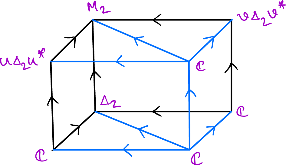
Consider the cube of finite von Neumann algebras depicted in Figure 1, where
 $A_1$
is equipped with a fixed faithful normal tracial state, such that
 $$ \begin{align} B_0^j=A_0\cap B_1^j\,,\,\,C_0=B_0^1\cap B_0^2\,,\,\,C_1=B_1^1\cap B_1^2 \end{align} $$
holds for
 $j=1,2$
. Note that in Figure 1, ‘
 $B\rightarrow A$
’ means
 $B\subseteq A$
. Recall the several equivalent conditions of a ‘commuting square’ from [Reference Jones and Sunder14, Definition 5.1.7].
Definition 3.1. We call the square
 $(C_0\subset A_0, C_1\subset A_1)$
of the cube in Figure 1 the slice of the cube.
Proposition 3.2. Suppose that the adjacent faces
 $$ \begin{align*} \begin{matrix} B_1^1 &\subset & A_1\\ \cup & &\cup & \\ B_0^1 &\subset & A_0\\ \end{matrix}\quad\mbox{and}\quad\begin{matrix} A_1 &\supset & B_1^2\\ \cup & &\cup & \\ A_0 &\supset & B_0^2\\ \end{matrix} \end{align*} $$
in Figure 1 are commuting squares. Then,
 $C_1\cap B_0^j=C_0$
for
 $j=1,2,$
and
 ${C_1\cap A_0=C_0}$
. Moreover, the remaining faces
 $(C_0\subset B_0^j\,,\,C_1\subset B_1^j),\,j=1,2$
are also commuting squares as is the slice
 $(C_0\subset A_0, \,C_1\subset A_1)$
.
Proof. Since
 $(B_0^j\subset A_0,B_1^j\subset A_1)$
are commuting squares for
 $j=1,2$
and
 $B_0^j=A_0\cap B_1^j$
by (3-1), we see that
 $A_0\cap C_1\subseteq A_0\cap B_1^j=B_0^j$
for
 $j=1,2$
. Thus,
 $A_0\cap C_1\subseteq B_0^1\cap B_0^1=C_0$
, and the converse is obvious. Then,
 $B_0^j\cap C_1\subseteq A_0\cap C_1=C_0$
for
 $j=1,2$
, and the converse is obvious. This completes the first part.
Now, recall that for a quadruple
 $(N\subset P,Q\subset M)$
, if
 $E^M_Q(P)\subseteq N$
(or
 $E^M_P(Q)\subseteq N$
), then it is a commuting square [Reference Jones and Sunder14]. Therefore, to show that the slice
 $(C_0\subset A_0,C_1\subset A_1)$
is a commuting square, it is enough to show that
 $E^{A_1}_{A_0}(c_1)\in C_0$
for all
 $c_1\in C_1$
. Since
 $C_1\subset B^1_1$
, by hypothesis, we have
 $E^{A_1}_{A_0}(c_1)\in B^1_0$
. Similarly, since
 $C_1\subset B^2_1$
, we get that
 $E^{A_1}_{A_0}(c_1)\in B^2_0$
. Hence,
 $E^{A_1}_{A_0}(c_1)\in C_0$
, which finishes the proof.
Cube of finite von Neumann algebras.

Finally, to show that the remaining faces of the cube are also commuting squares, it is enough to show that one is a commuting square; the other follows similarly. So, we consider one of the remaining faces
 $(C_0\subset B_0^1\,,\,C_1\subset B_1^1)$
and claim that
 $E^{B_1^1}_{B_0^1}(C_1)\subseteq C_0$
. Take any
 $x\in C_1$
and use the hypothesis that
 $(B_0^1\subset A_0,B_1^1\subset A_1)$
is a commuting square to observe the following:
 $$ \begin{align*} E^{B_1^1}_{B_0^1}(x)=E^{A_1}_{B_0^1}(x)=E^{A_1}_{A_0}E^{A_1}_{B_1^1}(x)=E^{A_1}_{A_0}(x). \end{align*} $$
Since the slice
 $(C_0\subset A_0,C_1\subset A_1)$
is already a commuting square, we get that
 $E^{A_1}_{A_0}(x)\in C_0$
, which concludes the proof.
Motivated by this result, we define the following notion.
Definition 3.3. A cube of finite von Neumann algebras depicted in Figure 1 is called a commuting cube if both the adjacent faces
 $(B_0^j\subset A_0,B_1^j\subset A_1),\,j=1,2,$
are commuting squares.
Pairs of spin model subfactors, to be discussed in the next section, provide natural examples of commuting cubes. The following remark is very important.
Remark 3.4.
-
(i) The floor and the roof in a commuting cube need not be commuting squares. We see examples in Section 5.
-
(ii) If the adjacent faces in a commuting cube are nondegenerate commuting squares, then although the slice
$(C_0\subset A_0,C_1\subset A_1)$
is a commuting square by Corollary 3.2, it may fail to become nondegenerate. The same applies to the remaining faces.

Proposition 3.5. Suppose that we have a commuting cube as depicted in Figure 1. If the roof
 $(C_1\subset B_1^1\,,\,B_1^2\subset A_1)$
is a commuting square, then the floor
 $(C_0\subset B_0^1\,,\,B_0^2\subset A_0)$
is also a commuting square.
Proof. Let
 $x\in B_0^1$
and observe the following:
 $$ \begin{align*} E^{A_0}_{B_0^2}(x) &= E^{A_0}_{B_0^2}E^{A_1}_{A_0}(x)\quad(\mbox{as }B_0^1\subset A_0)\\ &= E^{A_1}_{B_0^2}(x)\\ &= E^{A_1}_{B_1^2}E^{A_1}_{A_0}(x)\quad(\mbox{as }(B_0^2\subset A_0,B_1^2\subset A_1)\mbox{ is a commuting square})\\ &= E^{A_1}_{B_1^2}(x)\ \ \,\,\,\,\,\quad (\mbox{as }B_0^1\subset A_0)\\ &= E^{A_1}_{B_1^2}E^{A_1}_{B_1^1}(x)\quad(\mbox{as }x\in B_0^1\subset B^1_1)\\ &= E^{A_1}_{C_1}(x)\ \ \,\,\,\,\,\quad(\mbox{as }(C_1\subset B_1^1,B_1^2\subset A_1)\mbox{ is a commuting square}). \end{align*} $$
Since
 $x\in B_0^1\subseteq A_0$
and the slice
 $(C_0\subset A_0,C_1\subset A_1)$
is a commuting square by Corollary 3.2, we get that
 $E^{A_1}_{C_1}(x)\in C_0$
. This shows that
 $E^{A_0}_{B_0^2}(B_0^1)\subseteq C_0$
, which proves that the floor is also a commuting square.
The converse of the above result may not hold. We see an example in a moment. In general, the floor and the roof in a commuting cube need not be commuting squares. We see examples in Section 5 (Proposition 5.3 and Theorem 5.10 to be precise).
Definition 3.6. A commuting cube as depicted in Figure 1 is called a nondegenerate commuting cube if the adjacent faces and the slice are nondegenerate commuting squares.
An example. We give an example of a commuting cube that is degenerate. In this example, the adjacent faces are nondegenerate commuting squares, and the slice is a commuting square (due to Corollary 3.2) but degenerate. The same applies to the remaining faces. Consider two distinct
 $2\times 2$
complex Hadamard matrices
 $u\mbox { and }v$
of the following form:
 $$ \begin{align*} u=\frac{1}{\sqrt{2}}\,\left[{\begin{matrix} 1 & 1 \\ e^{i\alpha} & -e^{i\alpha} \\ \end{matrix}}\right] \quad\mbox{and}\quad v=\frac{1}{\sqrt{2}}\,\left[{\begin{matrix} 1 & 1 \\ e^{i\beta} & -e^{i\beta} \\ \end{matrix}}\right] \end{align*} $$
such that
 $\alpha -\beta \notin \{0,{\pi }/{2},-{\pi }/{2}\}$
. Obtain the cube as illustrated in Figure 2. In this cube, both the adjacent faces are nondegenerate commuting squares, since
 $u\mbox { and }v$
are complex Hadamard matrices. So, it is a commuting cube. Now, it is a straightforward verification that
 $\mbox {Ad}_u(\Delta _2)\cap \mbox {Ad}_v(\Delta _2)=\mathbb {C}$
. Hence, the quadruple
 $(\mathbb {C}\subset \mathbb {C},\Delta _2\subset M_2)$
, is a slice in the cube which is clearly not nondegenerate simply because the norm of the inclusion matrix
 $\Lambda ^{\Delta _2}_{\mathbb {C}}$
for the inclusion
 $\mathbb {C}\subset \Delta _2$
is
 $\sqrt {2}$
, whereas that of the inclusion matrix
 $\Lambda ^{M_2}_{\mathbb {C}}$
for the inclusion
 $\mathbb {C}\subset M_2$
is
 $2$
. The remaining faces are also not nondegenerate for a similar reason.
A degenerate commuting cube.

Also, note that in this example, the floor
 $(\mathbb {C}\subset \mathbb {C},\mathbb {C}\subset \Delta _2)$
is clearly a commuting square, but the roof
 $(\mathbb {C}\subset \mathrm {Ad}_u(\Delta _2),\mathrm {Ad}_v(\Delta _2)\subset M_2)$
is not a commuting square as there is a nontrivial ‘angle’ present (see Proposition 5.3 and Corollary 5.4 for the proof). Thus, the converse to Corollary 3.5 does not hold.
In Section 5, we encounter (nontrivial) examples of nondegenerate commuting cubes, where these ideas are extensively used.
Lemma 3.7. Suppose that we have two nondegenerate commuting squares
 $(B_1^j,A_1,B_2^j,A_2),\,j=1,2,$
of finite-dimensional algebras (see Figure 1 in this regard), and we obtain the following tower of nondegenerate commuting squares:
 $$ \begin{align*} \begin{matrix} A_1 &\subset & A_2 &\subset^{\,e_3} & A_3 &\subset^{\,e_4} &\cdots\\ \cup & & \cup & & \cup & & \\ B_1^j &\subset & B_2^j &\subset & B_3^j &\subset &\cdots \end{matrix} \end{align*} $$
through an iterated basic construction. That is,
 $A_k=\mathrm {Alg}\{A_{k-1},e_k\}$
for
 $k\geq 3$
, the algebra in
 $\mathcal {B}(L^2(A_{k-1}))$
generated by
 $A_{k-1}$
and
 $e_k$
, where
 $e_k$
is the Jones projection, and
 $B_k^j=\mathrm {Alg}\{B_{k-1}^j,e_k\}$
, the subalgebra of
 $A_k$
generated by
 $B_{k-1}^j$
and
 $e_k\in A_k$
. Let
 $C_k=\bigcap _{j=1}^2B_k^j$
for
 $k\geq 1$
and suppose that
 $(C_1\subset A_1,C_2\subset A_2)$
is a nondegenerate commuting square. Let
 $\,D_3=\mathrm {Alg}\{C_2,e_3\}$
and for
 $k\geq 4,\,D_k=\mathrm {Alg}\{D_{k-1},e_k\}$
. Then,
 $e_k\in C_k$
and
 $D_k\subseteq C_k$
for all
 $k\geq 3$
.
Proof. We omit the proof as it is an easy verification.
Basic construction of nondegenerate commuting cube. Consider the cube depicted in Figure 1 of finite-dimensional von Neumann algebras and assume that the adjacent faces
 $(B_0^j\subset A_0,B_1^j\subset A_1),\,j=1,2$
, are nondegenerate commuting squares. Suppose that the slice
 $(C_0\subset A_0,C_1\subset A_1)$
is also nondegenerate (see Remark 3.4). By Corollary 3.2, the slice is a commuting square, and such a cube is a nondegenerate commuting cube. Let
 $A_0\subset A_1\subset ^{\,e_2} A_2$
be an instance of the basic construction, where
 $e_2\in A_2$
is the Jones projection. Then,
 $C_2=\langle C_1,e_2\rangle $
and
 $B^j_2=\langle B_j^1,e_2\rangle $
are instances of basic constructions for the inclusions
 $C_0\subset C_1$
and
 $B^j_0\subset B^j_1$
, respectively, for
 $j=1,2$
. Moreover, we obtain the new cube depicted in Figure 3. The adjacent faces
 $(B_1^j\subset A_1,B_2^j\subset A_2),\,j=1,2$
, and the slice
 $(C_1\subset A_1,C_2\subset A_2)$
of the upper cube in Figure 3 remain nondegenerate commuting squares. Stacking the lower cube and the upper cube, we get a cube whose adjacent faces and the resulting slice
 $(C_0\subset A_0,C_2\subset A_2)$
are nondegenerate commuting squares. Iterating Jones’ basic construction, we (possibly) obtain a quadruple of
 $II_1$
factors
 $(N\subset P,Q\subset M)$
, where
 $M=\{\bigcup _{m\geq 0}\,A_m\}^{\prime \prime },\,P=\{\bigcup _{m\geq 0}\,B^1_m\}^{\prime \prime },\,Q=\{\bigcup _{m\geq 0}\,B^2_m\}^{\prime \prime }$
, and
 $N=\{\bigcup _{m\geq 0}\,C_m\}^{\prime \prime }$
. However, there is no guarantee that
 $P\neq Q$
a priori (Theorem 4.7 in the next section provides many instances of the situation
 $P=Q$
). If
 $P\mbox { and }Q$
are indeed distinct, with a little more effort, as in Lemma 3.7, we can conclude that
 $N\subseteq P\cap Q$
(note that
 $P\cap Q$
may not be a factor a priori, as discussed in Section 1 with the example that the intersection of two factors need not be a factor). Moreover,
 $[M:P]=||\Lambda ^{A_0}_{B^1_0}||^2$
(and similarly for Q) and
 $[M:N]=||\Lambda ^{A_0}_{C_0}||^2$
. By the Ocneanu compactness theorem, we have
 $N^{\,\prime }\cap M=C_1^{\,\prime }\cap A_0$
. Therefore, the iterated basic construction of a nondegenerate commuting cube of finite-dimensional algebras gives rise to a quadruple of factors.
Commuting cube and basic construction.

An instance of this construction is seen in Section 5. Corollary 3.5 has far-reaching consequences for two subfactors
 $P,Q\subset M$
obtained as iterated basic constructions of a nondegenerate commuting cube of finite-dimensional algebras. It says that if a nontrivial ‘angle’ (recall from Section 2) is present in the cube we start with, which is certainly computable being in finite dimensions, then the resulting quadruple
 $(N\subset P,Q\subset M)$
of
 $II_1$
factors is far from being a commuting square. We end this section with an application of a commuting cube.
Lemma 3.8. Consider the nondegenerate commuting cube depicted in Figure 1 and define the following operator:
 $$ \begin{align*} S_j:=E^{A_j}_{B^2_j}E^{A_j}_{B^1_j}E^{A_j}_{B^2_j}-E^{A_j}_{C_j} \end{align*} $$
for
 $j=0,1$
. Suppose that
 $S_0^{\,2}=\alpha S_0$
for some
 $\alpha \in \mathbb {R}_+$
. Then,
 $S_1^{\,2}=\alpha S_1$
.
Proof. Since the slice is nondegenerate by hypothesis, for any
 $x\in A_1$
, we have
 $x=\sum a_0c_1$
, where
 $a_0\in A_0$
and
 $c_1\in C_1$
. Then, the following holds:
 $$ \begin{align*} S_1(x)=(E_{B^2_1}E_{B^1_1}E_{B^2_1}-E_{C_1})(x) &= (E_{B^2_1}E_{B^1_1}E_{B^2_1}-E_{C_1})(\textstyle\sum a_0c_1)\\ &= E_{B^2_1}E_{B^1_1}(\textstyle\sum E_{B^2_1}(a_0)c_1)-\textstyle\sum E_{C_1}(a_0)c_1\\ &= \textstyle\sum\,E_{B^2_1}((E_{B^1_1}E_{B^2_1}(a_0))c_1)-\textstyle\sum E_{C_1}(a_0)c_1\\ &= \textstyle\sum(E_{B^2_1}E_{B^1_1}E_{B^2_1}-E_{C_1})(a_0)\,c_1\\ &= \textstyle\sum(E_{B^2_0}E_{B^1_0}E_{B^2_0}-E_{C_0})(a_0)\,c_1, \end{align*} $$
where the last line follows since
 $a_0\in A_0$
, and both the adjacent faces and the slice are commuting squares. This says
 $$ \begin{align*} S_1^{\,2}(x)=(E_{B^2_1}E_{B^1_1}E_{B^2_1}-E_{C_1})^2(\textstyle\sum a_0c_1)=\sum\,(E_{B^2_0}E_{B^1_0}E_{B^2_0}-E_{C_1})^2(a_0)\,c_1=\sum\,S_0^{\,2}(a_0)\,c_1, \end{align*} $$
which completes the proof.
Theorem 3.9. Suppose that
 $(N\subset P,Q\subset M)$
is a quadruple of
 $II_1$
factors obtained as an iterated basic construction of the nondegenerate commuting cube of finite-dimensional algebras depicted in Figure 1. Consider the nonnegative matrix
 $$ \begin{align*} S_0:=E^{A_0}_{B^2_0}E^{A_0}_{B^1_0}E^{A_0}_{B^2_0}-E^{A_0}_{C_0} \end{align*} $$
and suppose that
 $S_0\neq 0$
with
 $S_0^{\,2}=\alpha S_0$
for some
 $\alpha \in \mathbb {R}_+$
. Then,
 $(N\subset P,Q\subset M)$
is not a commuting square and, moreover, the set of angles (recall Definition 2.2)
 $\mathrm {Ang}_M(P,Q)$
is the singleton set
 $\{\mathrm {arccos}\sqrt {\alpha }\}$
.
Proof. Since
 $S_0\neq 0$
, the quadruple
 $(C_0\subset B^1_0,B^2_0\subset A_0)$
is not a commuting square. Therefore, none of the roofs, including the final one
 $(N\subset P,Q\subset M)$
, in the iterated basic construction (see Figure 3) are commuting squares due to Corollary 3.5. Since the basic construction of a nondegenerate commuting square is also so, we get that the resulting final slice
 $(C_0\subset A_0,N\subset M)$
is a nondegenerate commuting square, and so are the resulting final adjacent faces
 $(B^1_0\subset A_0,P\subset M)$
and
 $(B^2_0\subset A_0,Q\subset M)$
. Therefore, stacking all these nondegenerate commuting cubes, we obtain that the final commuting cube is nondegenerate. By Lemma 3.8, we obtain that
 $S_\infty :=E^M_PE^M_QE^M_P-E^M_N$
(and equivalently,
 $e_Pe_Qe_P-e_N$
) satisfies
 $S_\infty ^{\,2}=\alpha S_\infty $
. Since
 $S_\infty \neq 0$
and
 $\alpha>0$
, the result now follows from Lemma 2.3.
4 Pair of spin model subfactors: a general situation
Recall the construction of the spin model subfactors from Section 2. Let us begin at the beginning. Recall that any complex Hadamard matrix
 $U\in M_n$
induces the following nondegenerate commuting square:
 $$ \begin{align*} \begin{matrix} \Delta_n &\subset & M_n \cr \cup &\ & \cup\\ \mathbb{C} &\subset & U\Delta_nU^{*} \end{matrix} \end{align*} $$
and, iterating Jones’ basic construction, we obtain a spin model subfactor
 $R_U\subset R$
, where R is the hyperfinite type
 $II_1$
factor.
Definition 4.1. Given a nonzero vector
 $\mathbf {u}\in \mathbb {C}^n$
, the Hamming number is given by
 $$ \begin{align*} h(\mathbf{u}):=\mbox{number of nonzero entries in }\mathbf{u}. \end{align*} $$
Recall the Pimsner–Popa constant from Section 2. Our first result is the following.
Theorem 4.2. If
 $\Delta _n$
and
 $U\Delta _n U^{*}$
are two Masas in
 $M_n$
, the Pimsner–Popa probabilistic constant is given by
 $$ \begin{align*} \lambda(\Delta_n\,,\,U\Delta_n U^{*})=\min_{1\leq i\leq n}\,(h(U^{*})_i)^{-1}, \end{align*} $$
where
 $(U^{*})_i$
is the i th column of
 $U^{*}$
and
 $h(.)$
denotes the Hamming number.
We have the following immediate consequence. Recall from [Reference Popa23] that two von Neumann subalgebras
 $\mathcal {P,Q}$
of a fixed finite von Neumann algebra
 $(\mathcal {M},\tau )$
are called orthogonal, denoted by
 $\mathcal {P}\perp \mathcal {Q}$
, if
 $\tau (xy)=0$
for all
 $x\in \mathcal {P},y\in \mathcal {Q},\tau (x)=\tau (y)=0$
.
Corollary 4.3. The pair
 $(\Delta _n\,,\,U\Delta _nU^{*})$
in the type
 $I_n$
factor
 $M_n$
is an orthogonal pair in the sense of Popa only if the unitary U has no zero entry.
Proof. Let
 $(\Delta _n,\,U\Delta _nU^{*})$
be an orthogonal pair. Observe that
 $(\mathbb {C}\subset \Delta _n,\,U\Delta _n U^{*}\subset M_n)$
is a commuting square (see the last paragraph in [Reference Choda6, Section 1]). Hence,
 $h(\Delta _n|U\Delta _n U^{*})=H(\Delta _n|U\Delta _n U^{*})=H(\Delta _n|\mathbb {C})=\log n$
(apply [Reference Pimsner and Popa22]). Now by [Reference Choda6, Corollary 3.3], we know that
 $(\Delta _n,U\Delta _nU^{*})$
is an orthogonal pair in
 $M_n$
if and only if
 $h(\Delta _n|U\Delta _n U^{*})=\log n$
. Since
 $h(\Delta _n|U\Delta _n U^{*})\leq -\log \lambda (\Delta _n,U\Delta _n U^{*})$
by Proposition 2.18, we have the following inequalities:
 $$ \begin{align*} \log n=h(\Delta_n|U\Delta_n U^{*})\leq\log(\min_{1\leq i\leq n}\,h(U)_i)\leq\log n \end{align*} $$
by Theorem 4.2. Hence, all the entries of the unitary U must be nonzero.
Now, turning our attention back to Theorem 4.2, a bit of work is needed to prove this theorem. First, note that
 $\lambda (M_n,U\Delta _nU^{*})=\lambda (M_n,\Delta _n)={1}/{n}$
[Reference Pimsner and Popa22, Example in Section 6.5, page 94]. That is,
 $E_{U\Delta _nU^{*}}(x)\geq ({1}/{n})x$
for all
 $x\in (M_n)_+$
and, therefore,
 $\,\lambda (\Delta _n\,,\,U\Delta _n U^{*})\geq ({1}/{n})$
. The unique trace-preserving conditional expectation
 $\,E:M_n\rightarrow \Delta _n$
is given by
 $A\mapsto (a_{ii})_{ii}$
for any
 $A=(a_{ij})_{1\leq i,j\leq n}\in M_n$
. Here, the notation
 $(\,.\,)_{ii}$
denotes a diagonal matrix in
 $M_n$
. We are going to use the following well-known facts.
Weyl’s inequality for eigenvalues. Let
 $A\mbox { and }B$
be
 $n\times n$
self-adjoint matrices and
 $\widetilde {A}=A+B$
. Suppose that the eigenvalues of A are ordered as
 $\lambda _1(A)\leq \lambda _2(A)\leq \cdots \leq \lambda _n(A)$
, and similarly for the matrices
 $\widetilde {A}\mbox { and }B$
. Then,
 $$ \begin{align*}\lambda_k(A)+\lambda_1(B)\leq\lambda_k(\widetilde{A})\leq\lambda_k(A)+\lambda_n(B).\end{align*} $$
Matrix determinant lemma. Suppose A is an invertible
 $n\times n$
matrix and
 $\mathbf {u},\mathbf {v}$
are two vectors in
 $\mathbb {C}^n$
written as column matrices. Then,
 $$ \begin{align*} \det(A+\mathbf{u}\mathbf{v}^{\textsf{T}})=(1+\mathbf{v}^{\textsf {T}}A^{-1}\mathbf{u})\,\det(A). \end{align*} $$
By the definition of
 $\,\lambda $
, to find
 $\lambda (\Delta _n,U\Delta _n U^{*})$
, we need to find the best constant
 $t\in [0,1]$
in the following inequality:
 $$ \begin{align*} U(U^{*}xU)_{kk}U^{*}\geq tx\quad\text{for all } x\in(\Delta_n)_+. \end{align*} $$
This is because
 $E^{M_n}_{U\Delta _nU^{*}}=\mbox {Ad}_U\circ E^{M_n}_{\Delta _n}\circ \mbox {Ad}_{U^{*}}$
.
Lemma 4.4. For
 $1\leq i\leq n$
, consider the minimal projections
 $p_i:=E_{ii}$
in
 $M_n$
. Then,
 $$ \begin{align*} \lambda(\Delta\,,\,U\Delta U^{*})=\min_{1\leq i\leq n}\,\mathrm{sup}\,\{t\geq 0:(U^{*}p_iU)_{kk}\geq t\,U^{*}p_iU\}. \end{align*} $$
Proof. First, observe that
 $\Delta _n$
is generated by the minimal projections
 $p_i=E_{ii}$
in
 $M_n$
, and
 $U(U^{*}p_iU)_{kk}U^{*}\geq tp_i$
holds if and only if
 $(U^{*}p_iU)_{kk}\geq t\,U^{*}p_iU$
holds. Let us denote
 $$ \begin{align*} \widetilde{\lambda}_i:=\sup_{t\geq 0}\,\{(U^{*}p_iU)_{kk}\geq t\,U^{*}p_iU\} \end{align*} $$
for
 $\,i\in \{1,\ldots ,n\}$
. It is obvious from the definition of
 $\lambda $
that
 $\lambda (\Delta _n\,,\,U\Delta _nU^{*})\leq \widetilde {\lambda }_i$
for each i. Thus,
 $$ \begin{align*} \lambda(\Delta\,,\,U\Delta U^{*})\leq\min_{1\leq i\leq n}\,\widetilde{\lambda}_i. \end{align*} $$
Conversely, for any
 $x\in (\Delta _n)_+$
, we have
 $x=\sum _{i=1}^n\,\alpha _ip_i$
with all
 $\alpha _i\geq 0$
. Thus, for any
 $t\in [0,1],\,(U^{*}xU)_{kk}\geq t\,U^{*}xU$
holds if and only if the following inequality:
 $$ \begin{align} \sum_{i=1}^n\,\alpha_i(U^{*}p_iU)_{kk} \geq \sum_{i=1}^n\,\alpha_it\,U^{*}p_iU \end{align} $$
holds, and the best constant t satisfying the above inequality gives us
 $\lambda (\Delta \,,\,U\Delta U^{*})$
. Now, if we set
 $t_0=\min _{1\leq i\leq n}\,\widetilde {\lambda }_i$
, then by the definition of
 $\widetilde {\lambda }_i$
,
 $$ \begin{align*} (U^{*}p_iU)_{kk}\geq t_0\,U^{*}p_iU \end{align*} $$
for all i, and, consequently, (4-1) is satisfied for
 $t=t_0$
. By the definition of
 $\lambda $
,
 $$ \begin{align*} \lambda(\Delta\,,\,U\Delta U^{*})\geq t_0=\min_{1\leq i\leq n}\,\widetilde{\lambda}_i, \end{align*} $$
which completes the proof.
Let
 $\sigma =-t$
and for any fixed
 $i\in \{1,\ldots ,n\}$
, consider the following one-parameter family of
 $n\times n$
matrices:
 $$ \begin{align*} \{A_\sigma:=(U^{*}p_iU)_{kk}+\sigma\,U^{*}p_iU\,:\,\sigma\in[-1,0]\}. \end{align*} $$
Since
 $U^{*}p_iU$
is a rank-one matrix, any member of this family is a matrix of the form
 $D_\sigma +\sigma \,\mathbf {u}\mathbf {u}^{*}$
, where
 $\mathbf {u}\in \mathbb {C}^n$
is a vector written as a column matrix and
 $\mathbf {u}^{*}$
denotes the complex conjugate of the vector
 $\mathbf {u}$
written as a row matrix. Thus, any matrix
 $A_\sigma $
is a rank-
 $1$
perturbation of a diagonal matrix
 $D_\sigma $
. Throughout this subsection, we denote
 $U^{*}=(u_{ij}),\,1\leq i,j\leq n$
. We are interested in the following inequality:
 $$ \begin{align*}(U^{*}p_iU)_{kk}+\sigma U^{*}p_iU\geq 0,\end{align*} $$
that is,
 $$ \begin{align} \mbox{diag}(|u_{1i}|^2,\ldots,|u_{ni}|^2)+\sigma\,\left[{\begin{matrix} u_{1i}\\ \vdots\\ u_{ni}\\ \end{matrix}}\right] \begin{matrix} \left[{\begin{matrix} \overline{u_{1i}} & \cdots \overline{u_{ni}}\\ \end{matrix}}\right]\\[1.0ex] \\ \\ \end{matrix}\,\,\geq 0. \end{align} $$
Lemma 4.5. Except for possibly the minimum eigenvalue of the following self-adjoint matrix:
 $$ \begin{align*} \mathrm{diag}(|u_{1i}|^2,\ldots,|u_{ni}|^2)+\sigma\,\left[{\begin{matrix} u_{1i}\\ \vdots\\ u_{ni}\\ \end{matrix}}\right]\begin{matrix}\left[{\begin{matrix} \overline{u_{1i}} & \cdots & \overline{u_{ni}}\\ \end{matrix}}\right]\\[1.0ex] \\ \\ \end{matrix}, \end{align*} $$
all the other eigenvalues are nonnegative.
Proof. We write the matrix
 $A_\sigma $
as
 $P+D$
, where D is the diagonal matrix
 $\mbox {diag}(|u_{1i}|^2,\ldots ,|u_{ni}|^2)$
and P is the rank-one perturbation
 $A_\sigma -D$
. Since
 $({1}/{\sigma })P$
is a rank-
 $1$
projection, we have that the spectrum of P is given by
 $\sigma (P)=\{0,\sigma \}$
. We write the eigenvalues in increasing order as
 $$ \begin{align*} \lambda_1=\sigma\leq \lambda_2=\lambda_3=\cdots=\lambda_n=0. \end{align*} $$
Similarly, we write the eigenvalues of D in increasing order as
 $$ \begin{align*} 0\leq\mu_1\leq\mu_2\leq\cdots\leq\mu_n, \end{align*} $$
where we take
 $\mu _k=|u_{ki}|^2$
after possible renaming. Now, let the eigenvalues of
 $A_\sigma $
be
 $\widetilde {\lambda }_1\leq \cdots \widetilde {\lambda }_n$
. By Weyl’s inequality,
 $$ \begin{align*} \lambda_k+\mu_1\leq\widetilde{\lambda}_k\leq\lambda_k+\mu_n. \end{align*} $$
Putting
 $k=2$
, we get that
 $\widetilde {\lambda }_2\geq \lambda _2+\mu _1=\mu _1\geq 0$
. Thus,
 $\widetilde {\lambda }_k\geq 0$
for all
 $k=2,\ldots ,n$
, and this completes the proof.
Lemma 4.6. If all the entries of the unitary matrix U are nonzero, then
 $\lambda (\Delta \,,\,U\Delta U^{*})={1}/{n}$
.
Proof. Fix any
 $i\in \{1,\ldots ,n\}$
, and let
 $\mathbf {v}^T=(\overline {u_{1i}},\ldots ,\overline {u_{ni}})$
and
 $\mathbf {u}^T=(\sigma \,u_{1i},\ldots ,\sigma \,u_{ni}).$
Since,
 $u_{ij}\neq 0$
is given for all
 $i,j\in \{1,\ldots ,n\}$
, using the matrix determinant lemma,
 $$ \begin{align*} & \mbox{det}\left(\mbox{diag}(|u_{1i}|^2,\ldots,|u_{ni}|^2)+\sigma\,\left[{\begin{matrix} u_{1i}\\ \vdots\\ u_{ni}\\ \end{matrix}}\right]\begin{matrix}\left[{\begin{matrix} \overline{u_{1i}} & \cdots & \overline{u_{ni}}\\ \end{matrix}}\right]\\[1.0ex] \\ \\ \end{matrix}\right)\\ &\quad= \bigg(1+v^T\,\mbox{diag}\bigg(\frac{1}{|u_{1i}|^2},\ldots,\frac{1}{|u_{ni}|^2}\bigg)\,u\bigg)\,\mbox{det}\,\bigg(\mbox{diag}(|u_{1i}|^2,\,\ldots\,,|u_{ni}|^2)\bigg)\\ &\quad= \prod_{j=1}^n\,|u_{ji}|^2(1+n\sigma). \end{align*} $$
The quantity
 $\prod _{j=1}^n\,|u_{ji}|^2(1+n\sigma )$
is nonnegative if and only if
 $(1+n\sigma )$
is nonnegative. The matrix in (4-2) is positive semi-definite if and only if all its eigenvalues are nonnegative. Since all the
 $(n-1)$
eigenvalues, counted with multiplicities, are nonnegative by Lemma 4.5, we get that the best constant
 $\sigma \in [-1,0]$
in (4-2) is determined by the inequality
 $1+n\sigma \geq 0$
, since the determinant is the product of the eigenvalues. That is, the best constant
 $\sigma $
is given by
 $\sigma =-1/n$
and, consequently, the best constant t in the Pimsner–Popa constant is given by
 $t=1/n$
. Since this happens for any
 $1\leq i\leq n$
, by Lemma 4.4, we conclude the proof.
Proof of Theorem 4.2. Consider the i th column of
 $U^{*}$
for
 $1\leq i\leq n$
. Let
 $k_i$
be the number of zero elements in the set
 $\{u_{1i},\ldots ,u_{ni}\}$
. That is,
 $k_i$
many eigenvalues, counted with multiplicities, of the diagonal matrix
 $\,\mbox {diag}(|u_{1i}|^2,\ldots ,|u_{ni}|^2)$
are
 $0$
. Let
 $u_{j_1i}=\cdots =u_{j_{k_i}i}=0$
. Then, all the
 $j_\ell $
th rows for
 $1\leq \ell \leq k_i$
of the following
 $n\times n$
matrix:
 $$ \begin{align*} \left[{\begin{matrix} u_{1i}\\ \vdots\\ u_{ni}\\ \end{matrix}}\right]\begin{matrix}\left[{\begin{matrix} \overline{u_{1i}} & \cdots & \overline{u_{ni}}\\ \end{matrix}}\right]\\[1.0ex] \\ \\ \end{matrix} \end{align*} $$
are identically zero. Since
 $\overline {u_{j_1i}}=\cdots =\overline {u_{j_{k_i}i}}=0$
, all the
 $j_\ell $
th columns for
 $1\leq \ell \leq k$
of the above matrix are also identically zero. To obtain the Pimsner–Popa constant, we are interested in the best constant
 $\sigma \in [-1,0]$
for which (4-2) holds. That is, all the eigenvalues of the following matrix:
 $$ \begin{align*} A_\sigma=\mbox{diag}(|u_{1i}|^2,\ldots,|u_{ni}|^2)+\sigma\,\left[{\begin{matrix} u_{1i}\\ \vdots\\ u_{ni}\\ \end{matrix}}\right]\begin{matrix}\left[{\begin{matrix} \overline{u_{1i}} & \cdots & \overline{u_{ni}}\\ \end{matrix}}\right]\\[1.0ex] \\ \\ \end{matrix} \end{align*} $$
must be nonnegative. Since swapping two rows or columns only changes the sign of the determinant, the characteristic equation of the matrix
 $A_\sigma $
becomes
 $$ \begin{align*} 0 &= \mbox{det }(A_\sigma-xI_n)\\ &= \mbox{det }(\mbox{bl-diag }(-x,\ldots,-x,B_\sigma)), \end{align*} $$
where
 $B_\sigma $
is a
 $(n-k_i)\times (n-k_i)$
matrix. This says that positive semi-definiteness of
 $A_\sigma $
is completely determined by positive semi-definiteness of
 $B_\sigma $
. Now, observe that the matrix
 $B_\sigma $
is as in the earlier situation of Lemma 4.6, where all the entries of the following matrix:
 $$ \begin{align*} \mbox{diag}(\,|u_{j_{k_i+1}i}|^2,\ldots,|u_{j_ni}|^2) \end{align*} $$
are nonzero. Hence, the best constant
 $\sigma $
in (4-2) for the matrix
 $B_\sigma $
is given by
 ${\sigma =-{1}/({n-k_i})}$
. The number
 $n-k_i$
is exactly the number of nonzero entries in the i th column of
 $U^{*}$
. By Lemma 4.4, the proof is now complete.
A pair of spin model subfactors.

Now, consider a pair of distinct complex Hadamard matrices
 $u,v\in M_n$
and obtain the spin model subfactors
 $R_u,R_v\subset R$
depicted in Figure 4 (in the picture,
 $B\subset A$
is marked by
 $B\to A$
). Here,
 $u_0=u$
and
 $v_0=v$
by our convention, and
 $u_j$
(respectively,
 $v_j$
) are certain unitary matrices arising through basic constructions (see [Reference Nicoara20], for instance). However, it may happen that
 $R_u=R_v$
although
 $u\neq v$
, in which case, we fail to obtain a ‘pair’ of subfactors. Therefore, it is necessary to characterize which pairs
 $(u,v)$
of distinct complex Hadamard matrices give rise to pairs of spin model subfactors (see Problem 1.1 mentioned in Section 1).
Recall that a matrix in
 $GL_n(\mathbb {C})$
is said to be monomial (generalized permutation matrix) if each row and column has exactly one nonzero entry. Let N denote the set of all monomial matrices. It is known that N is a subgroup of
 $GL_n(\mathbb {C})$
and
 $N=\mathcal {N}_{GL_n}(\Delta _n)$
, the normalizer of
 $\Delta _n$
in
 $GL_n(\mathbb {C})$
. Consider the subgroup
 $\mathbb {G}:=N\cap U(n)$
of
 $GL_n(\mathbb {C})$
, where
 $U(n)$
is the set of all unitary matrices. Clearly,
 $\mathbb {G}$
consists of matrices with exactly one nonzero entry in each row and column, and this entry is of modulus one. Thus,
 $\mathbb {G}$
contains the set of all permutation matrices.
An equivalence relation. For unitary matrices
 $A,B\in M_n$
, consider the equivalence relation
 $A\sim B$
if
 $B=AC$
, where
 $C\in \mathbb {G}$
. Observe that
 $\mathbb {G}$
admits a right action on
 $M_n$
, and ‘
 $\sim $
’ is the orbit equivalence relation for this action. Recall that two complex Hadamard matrices
 $H_1,H_2$
are called Hadamard equivalent, denoted by
 $H_1\simeq H_2$
, if
 $H_2=D_1P_1H_1P_2D_2$
, where
 $D_1,D_2$
are unitary diagonal matrices and
 $P_1,P_2$
are permutation matrices. It is easy to check that ‘
 $\simeq $
’ is an equivalence relation, which follows from the fact that permutation matrices normalize the group of unitary diagonal matrices. Clearly, the equivalence relation ‘
 $\sim $
’ is finer than the Hadamard equivalence ‘
 $\simeq $
’. This is because the Hadamard equivalence
 $\simeq $
corresponds to orbits
 $\mathbb {G}H\mathbb {G},\,H\in M_n$
, whereas the equivalence relation
 $\sim $
corresponds to orbits
 $H\mathbb {G}$
.
With the help of this equivalence relation, we settle Problem 1.1 discussed in Section 1.
Theorem 4.7.
-
(i) For a pair of distinct complex Hadamard matrices
$u,v\in M_n$
, the pair of spin model subfactors
$R_u\subset R\mbox { and }R_v\subset R$
are distinct
$(R_u\neq R_v)$
if and only if
$\,u\nsim v$
. -
(ii) If a pair of complex Hadamard matrices
$u,v\in M_n$
are Hadamard inequivalent, then the corresponding spin model subfactors
$R_u\subset R\mbox { and }R_v\subset R$
are always distinct
$(R_u\neq R_v)$
.


Proof. For part (i), we prove the contrapositive, that is,
 $R_u=R_v$
if and only if
 $u\sim v$
. First, observe that
 $R_u=R_v$
if and only if
 $\lambda (R_u,R_v)=~1$
. This is because
 $\lambda (R_u,R_v)=1$
implies that
 $R_u\subseteq R_v$
by Lemma 2.13. Since
 $[R:R_u]=[R:R_v]=n$
, we get that
 $R_u=R_v$
. The converse direction is obvious.
Now, assume that
 $R_u=R_v$
. Then,
 $\lambda (R_u,R_v)=1$
and, consequently, we have
 ${\lambda (u\Delta _2u^{*}, v\Delta _2v^{*})=1}$
because
 $\lambda (R_u,R_v)$
is the limit of the decreasing sequence of
 $\lambda $
at each step of the tower of basic constructions (Proposition 2.14) and
 $0\leq \lambda \leq 1$
. By Theorem 4.2, we get that
 $u^{*}v$
must be a permutation matrix, that is,
 $u\sim v$
. Thus, we conclude that
 $R_u=R_v$
implies
 $u\sim v$
. Conversely, suppose that
 $u\sim v$
. Then,
 $v=uPD$
, where P is a permutation matrix in
 $M_n$
and
 $D\in U(n)$
is a diagonal unitary matrix. Then,
 $\mbox {Ad}_{u^{*}v}(\Delta _n)\subseteq \Delta _n$
and, consequently,
 $\mbox {Ad}_{v}(\Delta _n)\subseteq \mbox {Ad}_u(\Delta _n)$
. Immediately, we get that
 ${R_v\subseteq R_u}$
. Since
 $[R:R_u]=[R:R_v]=n$
, we get that
 $[R_u:R_v]=1$
and, hence,
 $R_u=R_v$
. This completes part (i), and part (ii) immediately follows from part (i), since the equivalence relation ‘
 $\sim $
’ is finer than the Hadamard equivalence relation.
Corollary 4.8. Let
 $u,v\in M_n$
be complex Hadamard matrices such that
 $u\nsim v$
. The Pimsner–Popa probabilistic constant
 $\lambda (R_u,R_v)$
satisfies the following bound:
 $$ \begin{align*} \lambda(R_u,R_v)\leq \min_{1\leq i\leq n}(h(v^{*}u)_i)^{-1}, \end{align*} $$
where
 $(v^{*}u)_i$
is the i th column of the unitary matrix
 $\,v^{*}u\in M_n$
and
 $h(.)$
denotes the Hamming number.
5 Spin model subfactors corresponding to
$\mathbb {Z}_2$
-actions

The goal of this section is to investigate Problems 1.2 and 1.3 discussed in Section 1 in depth for spin model subfactors corresponding to
 $\mathbb {Z}_2$
-actions. We observe a few curious phenomena in this ‘ground case’ itself.
Recall that
 $2\times 2$
complex Hadamard matrices form a single family up to Hadamard equivalence, and any element of this family is given by
 $$ \begin{align} F^{\alpha_1}_{\alpha_2}(\alpha_3):=\frac{1}{\sqrt{2}} \begin{bmatrix} e^{i\alpha_1} & e^{i (\alpha_1+\alpha_3)}\\ e^{i\alpha_2} & -e^{i(\alpha_2+\alpha_3)} \end{bmatrix}, \end{align} $$
where
 $\alpha _j\in [0,2\pi ),\,j=1,2,3$
. Also recall the equivalence relation ‘
 $\sim $
’ from Theorem 4.7. Consider any two
 $2\times 2$
complex Hadamard matrices u and v such that
 $u\nsim v$
, and obtain the pair of irreducible subfactors
 $R_u\subset R\mbox { and }R_v\subset R$
, each with index
 $2$
.
Note that
 $u\nsim v$
if and only if
 $v\neq uPD$
, where D is a diagonal unitary matrix and P is a permutation matrix. In this
 $2\times 2$
situation, we have that
 $PD$
is a unitary matrix of the form
 $[{\begin {smallmatrix} \alpha & 0\\ 0 & \beta \\ \end {smallmatrix}}]$
or
 $[{\begin {smallmatrix} 0 & \alpha \\ \beta & 0\\ \end {smallmatrix}}],$
where
 $\alpha ,\beta \in \mathbb {S}^1$
. Given any
 $u=F^{\alpha _1}_{\alpha _2}(\alpha _3)$
and
 $v=F^{\beta _1}_{\beta _2}(\beta _3)$
described in (5-1), consider the following matrices:
 $$ \begin{align*} \widetilde{u}=\frac{1}{\sqrt{2}}\begin{bmatrix} 1 & 1\\ e^{i(\alpha_2-\alpha_1)} & -e^{i(\alpha_2-\alpha_1)} \end{bmatrix}\quad\mbox{and}\quad\widetilde{v}=\frac{1}{\sqrt{2}}\begin{bmatrix} 1 & 1\\ e^{i(\beta_2-\beta_1)} & -e^{i(\beta_2-\beta_1)} \end{bmatrix} \end{align*} $$
associated to them. Since
 $u\sim \widetilde {u}$
, by Theorem 4.7, we have
 $R_u=R_{\widetilde {u}}$
, and similarly for v. Hence, the quadruples
 $(R_u\cap R_v\subset R_u,R_v\subset R)$
and
 $(R_{\widetilde {u}}\cap R_{\widetilde {v}}\subset R_{\widetilde {u}},R_{\widetilde {v}}\subset R)$
of von Neumann algebras are the same. Therefore, without loss of generality, throughout the section, we can and do assume that
 $$ \begin{align} u=\frac{1}{\sqrt{2}} \begin{bmatrix} 1 & 1\\ e^{i\alpha} & -e^{i\alpha} \end{bmatrix}\quad\mbox{and}\quad v=\frac{1}{\sqrt{2}} \begin{bmatrix} 1 & 1\\ e^{i\beta} & -e^{i\beta} \end{bmatrix} \end{align} $$
for
 $\alpha ,\beta \in [0,2\pi )$
. Note that
 $\beta =\alpha \pm \pi $
implies that
 $v=u\sigma _1$
, which gives
 $u\sim v$
. Therefore, in our situation, we have
 $\alpha ,\beta \in [0,2\pi )$
with
 $\beta \neq \alpha ,\alpha \pm \pi $
.
Note that
 $$ \begin{align*} \mathbb{C}\subset \Delta_2\subset M_2\subset \Delta_2 \otimes M_2\subset M_2\otimes M_2\subset \Delta_2\otimes M_2\otimes M_2\subset M_2\otimes M_2\otimes M_2\subset\cdots \end{align*} $$
is a tower of Jones’ basic construction and R is the closure in the strong operator topology of the union of these subalgebras. Starting with
 $u\mbox { and }v$
as in (5-2), we obtain a pair of spin model subfactors as depicted in Figure 4 in Section 4 (put
 $n=2$
). Although the basic construction (in the general
 $n\times n$
case) is well known (see [Reference Jones13, Reference Jones and Sunder14] and [Reference Nicoara20], for instance), our basic construction is slightly different from that in the existing literature as it is more handy in the subsequent computations.
To fix notation, let
 $u=(u_{ij})$
be a
 $2\times 2$
complex Hadamard matrix and consider the associated matrices
 $$ \begin{align*} \eta=\left[{\begin{matrix} \dfrac{u_{12}}{u_{11}} & 0\\[8pt] 0 & \dfrac{u_{22}}{u_{21}}\\ \end{matrix}}\right]\quad \mbox{and}\quad \xi=\frac{1}{\sqrt{2}}\,\left[{\begin{matrix} 1 & \dfrac{u_{12}}{u_{11}}\\[8pt] 1 & \dfrac{u_{22}}{u_{21}}\\ \end{matrix}}\right]. \end{align*} $$
Since u is unitary, it is easy to check that
 $\,\eta \mbox { and }\xi $
are unitary matrices. Let
 $I_2^{(k)}$
denote the unit element
 $I_2\otimes \cdots \otimes I_2$
in
 $(M_2)^{\otimes \,k}$
. We have the following tower of basic construction (with the convention
 $u_0=u$
).
Theorem 5.1. The tower of the basic construction for
 $\mathbb {C}\subset u\Delta _2u^{*}$
is given by
 $$ \begin{align*} \mathbb{C}\subset u_0\Delta_2u^{*}_0\subset u_1M_2u^{*}_1\subset u_2(\Delta_2\otimes M_2)u^{*}_2\subset u_3(M_2\otimes M_2)u^{*}_3\subset\cdots, \end{align*} $$
where each
 $u_i$
is a unitary matrix given by the following:
-
(i) for
$k\in \mathbb {N}$
, we have
$\,u_{2k}=u_{2k-1}(\xi _k\otimes I_2^{(k)})$
, where and
$$ \begin{align*} \xi_k &= \begin{cases} \xi^{*} & \mbox{if } k=1, \cr F_2 & \mbox{if } k\geq 2, \cr \end{cases} \end{align*} $$
$\,F_2={1}/\kern -2pt{\sqrt {2}}\, [{\begin {smallmatrix} 1 & 1\\ 1 & -1\\ \end {smallmatrix}}]$
is the Fourier matrix in
$M_2$
;
-
(ii) for
$k\in \mathbb {N}\cup \{0\}$
, we have
$\,u_{2k+1}=(I_2\otimes u_{2k})(E_{11}\otimes I_2^{(k+1)}+E_{22}\otimes \eta _k)$
, where and
$$ \begin{align*} \eta_k &= \begin{cases} \eta & \mbox{if }k=0, \cr \sigma_3\otimes I_2^{(k)} & \mbox{if } k\geq 1, \cr \end{cases} \end{align*} $$
$\sigma _3$
is a Pauli spin matrix described in Section 1.1.


The proof of the above theorem is a routine verification using induction, and interested readers are requested to visit the Appendix in arXiv:2212.07197 for details.
5.1 Factoriality of the intersection
In this subsection, we prove that
 $R_u\cap R_v$
is a
 $II_1$
subfactor of R with
 $[R:R_u\cap R_v]$
=4. We also characterize when the quadruple
 $(R_u\cap R_v\subset R_u,R_v\subset R)$
of
 $II_1$
factors is a commuting (and co-commuting) square. Recall the Pauli spin matrices from Section 1.1, which we use here frequently. Also, for the sake of brevity, we introduce the following notation.
Notation 5.2.
-
(1) For
$k\in \mathbb {N}\cup \{0\}$
, let These are the even steps in the tower of basic constructions in Figure 4. Note that
$$ \begin{align*} A_{2k} &= M_2\otimes M_2^{(k)},\cr B^u_{2k} &= u_{2k}(\Delta_2\otimes M_2^{(k)})u_{2k}^{*},\cr B^v_{2k} &= v_{2k}(\Delta_2\otimes M_2^{(k)})v_{2k}^{*},\cr C_{2k} &= B^u_{2k}\cap {B}^v_{2k}. \end{align*} $$
$$ \begin{align*} \overline{\bigcup_k\,A_{2k}}^{\mbox{ sot}}=R,\,\,\overline{\bigcup_k\,B^u_{2k}}^{\mbox{ sot}}=R_u,\,\,\overline{\bigcup_k\,B^v_{2k}}^{\mbox{ sot}}=R_v\,\mbox{ and }\,\overline{\bigcup_k\,C_{2k}}^{\mbox{ sot}}=R_u\cap R_v. \end{align*} $$
-
(2) For
$k\in \mathbb {N}$
, let
$W_{2k}:=E_{11}\otimes I_2^{(k)}+E_{22}\otimes \sigma _1^{(k)}$
in
$\Delta _2\otimes M_2^{(k)}$
. Each
$W_{2k}$
is unitary in
$M_2^{(k+1)}$
. Recall that
$A^{(k)}\in M_2^{(k)}$
denotes the matrix
$A^{\otimes \,k}=A\otimes A\otimes \cdots \otimes A$
in
$M_2^{(k)}$
.


We begin with the Sano–Watatani angle between
 $B^u_0\mbox { and }B^v_0$
(see Notation 5.2), and show that the following quadruple:
 $$ \begin{align} \begin{matrix} B^u_0 &\subset & A_0\\ \cup & & \cup\\ C_0 &\subset & B^v_0\\ \end{matrix} \end{align} $$
is not always a commuting square. This is an example which shows that the floor (and consequently the roof due to Corollary 3.5) in Figure 1 need not be a commuting square. The difficulty starts from here.
Proposition 5.3. If
 $u= {1}/\kern -2pt{\sqrt {2}}[\begin {smallmatrix} e^{i\alpha _1} & e^{i (\alpha _1+\alpha _3)}\\ e^{i\alpha _2} & -e^{i(\alpha _2+\alpha _3)} \end {smallmatrix}]$
and
 $v= {1}/\kern -2pt{\sqrt {2}}[\begin {smallmatrix} e^{i\beta _1} & e^{i (\beta _1+\beta _3)}\\ e^{i\beta _2} & -e^{i(\beta _2+\beta _3)} \end {smallmatrix}]$
, then the cosine of the angle between
 $u\Delta _2u^{*}\mbox { and }v\Delta _2v^{*}$
is the set
 $\{0,|\!\cos ((\alpha _1-\alpha _2)-(\beta _1-\beta _2))|\}$
, and the quadruple in (5-3) is a commuting square if and only if
 $\alpha _1-\alpha _2=\beta _1-\beta _2\pm ({\pi }/{2})$
.
Proof. It is clear that
 $u\Delta _2u^{*}\cap \,v\Delta _2v^{*}=\mathbb {C}$
, as
 $\mbox {dim}(u\Delta _2u^{*})=\mbox {dim}(v\Delta _2v^{*})=2$
and
 $u\Delta _2u^{*}=v\Delta _2v^{*}$
implies that
 $u\sim v$
by Theorem 4.2. Consider the nonnegative operator
 $E_{u\Delta _2u^{*}}E_{v\Delta _2v^{*}}E_{u\Delta _2u^{*}}$
, and observe that as an element of
 $\mathcal {B}(M_2,tr)=M_4$
, this is the same as the operator
 $\mbox {Ad}_uE_{\Delta _2}\mbox {Ad}_{u^{*}}\mbox {Ad}_vE_{\Delta _2}\mbox {Ad}_{v^{*}}\mbox {Ad}_uE_{\Delta _2}\mbox {Ad}_{u^{*}}$
. Put
 $w=(w_{ij})=u^{*}v$
, a unitary in
 $M_2$
. Then, we have the operator
 $\mbox {Ad}_uE_{\Delta _2} E_{w\Delta _2w^{*}}E_{\Delta _2}\mbox {Ad}_{u^{*}}$
in
 $\mathcal {B}(M_2)$
. First, consider
 $E_{\Delta _2}E_{w\Delta _2w^{*}}E_{\Delta _2}\in \mathcal {B}(M_2)$
. Since w is a
 $2\times 2$
unitary matrix, we have
 $|w_{12}|^2=|w_{21}|^2$
. We put
 $c= \sum _{i=1}^2{|w_{1i}|}^4$
and
 $s= {2}\prod _{i=1}^2 {|w_{i1}|}^2$
. It is easy to observe that
 $\sum _{i=1}^2 {|w_{2i}|}^4=c$
and
 $2\prod _{i=1}^2 {|w_{i2}|}^2=s$
. Therefore, using the fact that
 $|w_{11}|^2+|w_{12}|^2=1$
(as
 $w^{*}$
is a unitary),
 $$ \begin{align*} c+s=|w_{11}|^4+|w_{12}|^4+ 2|w_{11}|^2|w_{21}|^2=|w_{11}|^4+|w_{12}|^4+ 2|w_{11}|^2|w_{12}|^2=1. \end{align*} $$
Now, it is easy to verify that
 $$ \begin{align*} E_{\Delta} E_{w\Delta w^{*}} E_{\Delta}(A)=\mathrm{diag}\{c a_{11}+ (1-c) a_{22}\,,\,(1-c) a_{11}+ c a_{22}\} \end{align*} $$
for any matrix
 $A=(a_{ij})$
in
 $M_2$
. Therefore, with respect to the ordered orthonormal basis
 $\mathfrak {B}:=\{\sqrt {2}E_{11},\sqrt {2}E_{22},\sqrt {2}E_{12},\sqrt {2}E_{21}\}$
of
 $M_2$
, the operator
 $E_{\Delta _2}E_{w\Delta _2 w^{*}}E_{\Delta _2}:M_2\longrightarrow M_2$
, when viewed as a linear map from
 $\mathbb {C}^{4}$
to
 $\mathbb {C}^{4}$
, is of the form
 $\mbox {bl-diag}\{C,0\}$
, where
 ${C}= [\begin {smallmatrix} c & 1-c \\ 1-c &~ c \end {smallmatrix}]$
. The conditional expectation from
 $M_2$
onto
 $u\Delta _2u^{*}\cap v\Delta _2v^{*}$
is simply the trace
 $tr$
. Therefore, with respect to the ordered orthonormal basis
 $\mathfrak {B}$
, the operator
 $tr:M_2\to \mathbb {C}\subset M_2$
given by
 $A\mapsto tr(A)I_2$
is of the form
 $\mbox {bl-diag}\{J_2,0\}$
, where
 $J_2$
is the projection
 $\tfrac 12\sum _{i,j=1}^2E_{ij}$
in
 $M_2$
. Hence,
 $E_{u\Delta _2u^{*}}E_{v\Delta _2v^{*}}E_{u\Delta _2u^{*}}-tr$
has the form
 $\mbox {bl-diag}\{C-J_2,0\}$
. The quadruple in (5-3) is a commuting square if and only if
 $E_{u\Delta _2u^{*}}E_{v\Delta _2v^{*}}E_{u\Delta _2u^{*}}-tr$
, that is,
 $C=J_2$
. Since
 $J_2=\tfrac 12\sum _{i,j=1}^2 E_{ij}$
, we see that
 $C=J_2$
holds if and only if
 $c=s=\tfrac 12$
. A straightforward verification leads us to
 $c=\tfrac 12(1+\cos ^2(\beta _1-\alpha _1-\beta _2+\alpha _2))$
. Therefore, the quadruple in (5-3) is a commuting square if and only if
 $\alpha _1-\alpha _2=\beta _1-\beta _2\pm ({\pi }/{2})$
.
Now, suppose that this condition is not satisfied. The spectrum of the operator
 $\mbox {Ad}_u(E_{\Delta _2}E_{w\Delta _2 w^{*}} E_{\Delta _2} - tr)\mbox {Ad}_{u^{*}}$
is simply the spectrum of the matrix
 $C-J_2\in M_2$
. This is because
 $\mbox {Ad}_u\in \mathcal {B}(M_2)$
is a unitary. Therefore, the spectrum of the operator
 $E_{u\Delta _2u^{*}}E_{v\Delta _2v^{*}}E_{u\Delta _2u^{*}}-E_{u\Delta _2u^{*}\,\cap \,v\Delta _2v^{*}}$
is the spectrum of the matrix
 $C-J_2$
, which is the set
 $\{0,2c\kern1.4pt{-}\kern1.4pt1\}$
. Observe that
 $2c\kern1.4pt{-}\kern1.4pt1\kern1.4pt{=}\kern1.4pt({|w_{11}|}^2\kern1.4pt{-}\kern1.4pt{|w_{12}|}^2)^2$
. A straightforward verification shows that
 $|w_{11}|^2-|w_{12}|^2=\cos ((\alpha _1-\alpha _2)-(\beta _1-\beta _2))$
. Therefore, we obtain that cosine of the angle between
 $u\Delta _2u^{*}\mbox { and }v\Delta _2v^{*}$
is the set
 $\{0,|\!\cos ((\alpha _1-\alpha _2)-(\beta _1-\beta _2))|\}$
.
Corollary 5.4. Let
 $\,u\mbox { and }v$
be of the form described in (5-2). Then, the cosine of the angle between
 $\mathrm {Ad}_u(\Delta _2)\mbox { and }\mathrm {Ad}_v(\Delta _2)$
is the set
 $\{0,|\!\cos (\alpha -\beta )|\}$
.
By Corollary 5.4, the quadruple
 $(C_0\subset B^v_0\,,\,B^u_0\subset A_0)$
in (5-3), and consequently
 $(R_u\cap R_v\subset R_u,R_v\subset R)$
due to Corollary 3.5, is not a commuting square unless
 $\alpha -\beta =\pm ({\pi }/{2})$
. With the notation as in Theorem 5.1, we now identify the finite-dimensional grid
 $C_{2k}$
for
 $R_u\cap R_v$
.
Lemma 5.5. We have
 $$ \begin{align*} {u}^{*}_{2k}{v}_{2k} (\Delta_2\otimes M^{(k)}_2){v}^{*}_{2k}{u}_{2k} =W_{2k}(u^{*}v\Delta_2v^{*}u\otimes M^{(k)}_2) W^{*}_{2k} \end{align*} $$
for any
 $k\in \mathbb {N}$
, where
 $W_{2k}$
is as defined in Notation 5.2.
Proof. We first prove it for
 $k=1$
. We have
 $$ \begin{align} u^{*}v = \tfrac{1}{2}(1+e^{i(\beta-\alpha)})I_2+\tfrac{1}{2}(1-e^{i(\beta-\alpha)})\sigma_1. \end{align} $$
Applying Theorem 5.1,
 $$ \begin{align*} u^{*}_2v_2=\frac{1}{2}\begin{bmatrix} u^{*}v+\sigma_3u^{*}v\sigma_3 & u^{*}v-\sigma_3u^{*}v\sigma_3\\ u^{*}v+\sigma_3u^{*}v\sigma_3 & u^{*}v-\sigma_3u^{*}v\sigma_3 \end{bmatrix}. \end{align*} $$
Note that
 $$ \begin{align*} u^{*}v+\sigma_3u^{*}v\sigma_3=(1+e^{i(\beta-\alpha)})I_2\quad\mbox{ and }\quad u^{*}v-\sigma_3u^{*}v\sigma_3=(1-e^{i(\beta-\alpha)})\sigma_1. \end{align*} $$
Therefore,
 $$ \begin{align} u^{*}_2v_2=\tfrac{1}{2}(1+e^{i(\beta-\alpha)})I_2\otimes I_2+\tfrac{1}{2}(1-e^{i(\beta-\alpha)})\sigma_1\otimes\sigma_1. \end{align} $$
 $$ \begin{align*} u^{*}_2v_2=\mbox{bl-diag}\{I_2,\sigma_1\}(u^{*}v\otimes I_2)\mbox{bl-diag}\{I_2,\sigma_1\}, \end{align*} $$
and hence,
 $$ \begin{align*} u^{*}_2v_2(\Delta_2\otimes M_2)v^{*}_2u_2=\mbox{bl-diag}\{I_2,\sigma_1\}(u^{*}v\Delta_2v^{*}u\otimes M_2) \mbox{bl-diag}\{I_2,\sigma_1\}. \end{align*} $$
To complete the induction, note that for
 $k\geq 2$
, thanks to Theorem 5.1,
 $$ \begin{align*} u^{*}_{2k}v_{2k}=\tfrac{1}{2}(1+e^{i(\beta-\alpha)})I_2^{(k)}+\tfrac{1}{2}(1-e^{i(\beta-\alpha)})\sigma_1^{(k)}. \end{align*} $$
In other words, by (5-4),
 $$ \begin{align*} u^{*}_{2k}v_{2k}=\mbox{bl-diag}\{I^{(k)}_2,\sigma_1^{(k)}\}(u^{*}v\otimes I^{(k)}_2)\mbox{bl-diag}\{I^{(k)}_2,\sigma_1^{(k)}\}. \end{align*} $$
Since
 $W_{2k}=\mbox {bl-diag}\{I^{(k)}_2,\sigma _1^{(k)}\}\in \Delta _2\otimes M^{(k)}_2$
, the proof is complete.
Proposition 5.6. For any
 $k\in \mathbb {N}$
,
 $$ \begin{align*} C_{2k}:=u_{2k}(\Delta_2\otimes M_2^{(k)})u_{2k}^{*}\bigcap v_{2k}(\Delta_2\otimes M_2^{(k)})v_{2k}^{*} &= \mathrm{Ad}_{u_{2k}W_{2k}}((\Delta_2\cap (u^{*}v\Delta_2v^{*}u))\otimes M_2^{(k)})\\ &= \mathrm{Ad}_{u_{2k}W_{2k}}(\mathbb{C}\otimes M_2^{(k)}). \end{align*} $$
Proof. We have
 $$ \begin{align*} & u_{2k}(\Delta_2\otimes M_2^{(k)})u_{2k}^{*}\bigcap v_{2k}(\Delta_2\otimes M_2^{(k)})v_{2k}^{*}\\ &\quad= \mbox{Ad}_{u_{2k}}\bigg(\Delta_2\otimes M_2^{(k)}\bigcap \mbox{Ad}_{u_{2k}^{*}v_{2k}}(\Delta_2\otimes M_2^{(k)})\bigg)\\ &\quad= \mbox{Ad}_{u_{2k}}\bigg(\Delta_2\otimes M_2^{(k)}\bigcap \mbox{Ad}_{W_{2k}}(u^{*}v\Delta_2v^{*}u\otimes M_2^{(k)})\bigg)\quad(\mbox{by Lemma}~{5.5})\\ &\quad= \mbox{Ad}_{u_{2k}W_{2k}}\bigg(\Delta_2\otimes M_2^{(k)}\bigcap\, (u^{*}v\Delta_2v^{*}u)\otimes M_2^{(k)}\bigg)\\ &\quad= \mbox{Ad}_{u_{2k}W_{2k}}((\Delta_2\cap\,(u^{*}v\Delta_2v^{*}u))\otimes M_2^{(k)}). \end{align*} $$
This proves the first equality, and for the second, note that since
 $\beta \neq \alpha ,\pi \pm \alpha $
in our case, we have
 $\Delta _2\cap (u^{*}v\Delta _2v^{*}u)=\mathbb {C}$
.
We have the following tower of finite von Neumann algebras:
 $$ \begin{align*} \begin{matrix} A_0 &\subset & A_2 &\subset & A_4 &\subset &\cdots &\subset & R \cr \cup & &\cup & &\cup & & \cdots & &\cup \cr B_0^u &\subset & B_2^u &\subset & B_4^u &\subset &\cdots &\subset & R_u \cr \cup & &\cup & &\cup & &\cdots & &\cup \cr C_0 &\subset & C_2 &\subset & C_4 &\subset &\cdots &\subset & R_u\cap R_v \end{matrix} \end{align*} $$
Lemma 5.7. In the following diagram:
 $$ \begin{align*} \begin{matrix} A_0 &\subset & A_2 &\subset & A_4 &\subset &\cdots &\subset & R \cr \cup & &\cup & &\cup & & \cdots & & \cup \cr C_0 &\subset & C_2 &\subset & C_4 &\subset &\cdots &\subset & R_u\cap R_v \end{matrix} \end{align*} $$
each individual quadruple is a commuting square.
Commuting cube
 $\mathscr {C}_k$
.

Proof. Choose any
 $k\in \mathbb {N}$
and consider the quadruple
 $(C_{2k-2}\subset C_{2k}\,,\,A_{2k-2}\subset A_{2k})$
. Draw the cube
 $\mathscr {C}_k$
depicted in Figure 5. Here, by the construction of spin model subfactors
 $R_u\subset R$
and
 $R_v\subset R$
, respectively, the adjacent faces
 $(B^u_{2k-2}\subset A_{2k-2}, B^u_{2k}\subset A_{2k})$
and
 $(B^v_{2k-2}\subset A_{2k-2}\,,\,B^v_{2k}\subset A_{2k})$
are commuting squares. Since the required quadruple is the slice in Figure 5, by Corollary 3.2, it is a commuting square.
Theorem 5.8. The von Neumann subalgebra
 $R_u\cap R_v$
of R is a
 $II_1$
subfactor with
 $[R:R_u\cap R_v]=4$
and
 $[R_u:R_u\cap R_v]=[R_v:R_u\cap R_v]=2$
.
Proof. By Proposition 5.6, we have
 $C_0=\mathbb {C}$
and
 $C_2=\mbox {Ad}_{u_2W_2}(\mathbb {C}\otimes M_2)$
. In Lemma 5.7, putting
 $k=1$
, we have the following commuting square denoted by the symbol
 $\mathscr {S}$
:
 $$ \begin{align*} \begin{matrix} \mathbb{C}\otimes M_2 &\subset & M_2\otimes M_2 \cr \cup & &\cup \cr \mathbb{C} &\subset & \mbox{Ad}_{u_2W_2}(\mathbb{C}\otimes M_2) \end{matrix} \end{align*} $$
which is the slice in the commuting cube
 $\mathscr {C}_1$
depicted in Figure 5. Observe that the norms of the inclusion matrices of both the vertical embeddings in
 $\mathscr {S}$
are the same and equal to
 $2$
. Therefore,
 $\mathscr {S}$
is a nondegenerate commuting square. In other words, the slice in the commuting cube
 $\mathscr {C}_1$
is nondegenerate and, hence, the commuting cube
 $\mathscr {C}_1$
is a nondegenerate commuting cube by Definition 3.6. The tower of the basic construction for the horizontal inclusion
 $\mathbb {C}\otimes M_2\subset M_2\otimes M_2$
in
 $\mathscr {S}$
is given by
 $$ \begin{align} \hspace{-10pt}\mathbb{C}\otimes M_2 \subset M_2\otimes M_2 \subset^{f_1} {M}^{(2)}_2 \otimes M_2\subset^{f_2} {M}^{(3)}_2\otimes M_2\subset\cdots \subset^{f_k} {M}^{(k)}_2\otimes M_2\subset\cdots,\quad \end{align} $$
where
 $f_k=\tfrac 12\sum _{i,j=1}^{2}E_{ij}\otimes E_{ij}\otimes I^{(k)}_2\in M^{(k+1)}_2\otimes M_2=M^{(k+2)}_2$
is the Jones projection. Indeed, by our construction in Figure 4, we have the following tower:
 $$ \begin{align*} \mathbb{C}\subset\Delta_2\subset^{\,e_1} M_2\subset^{\,e_2}\Delta_2\otimes M_2\subset^{\,e_1\otimes I_2\,} M_2\otimes M_2\subset^{\,e_2\otimes I_2\,}\Delta_2\otimes M_2\otimes M_2\subset\cdots\subset R \end{align*} $$
for the hyperfinite factor R, where
 $e_1=J_2,\,e_2=\mbox {diag}\{E_{11},E_{22}\}$
. Applying [Reference Bakshi1, Theorem 3.5], for instance, we obtain the above form for
 $f_k$
. We put
 $L_{-1}=\mathbb {C}$
and set
 ${L_0= \mbox {Ad}_{u_2W_2} (\mathbb {C}\otimes M_2)}$
, and for
 $k \geq 1$
, suppose that
 $L_k=\{L_{k-1},f_k\}^{\prime \prime }$
. As
 $\mathscr {S}$
is a nondegenerate commuting square, it follows that the following tower of algebras is the Jones basic construction tower:
 $$ \begin{align*} \mathbb{C}\subset L_0\subset L_1\subset^{f_2} L_2 \subset \cdots \subset^{f_k} L_k\subset\cdots. \end{align*} $$
Define
 $R_{u,v}=\overline {\bigcup _k L_k}^{\tiny \,\mbox {sot}}$
. Note that
 $R_{u,v}$
is a
 $II_1$
subfactor of R with
 $[R:R_{u,v}]=4$
(see [Reference Jones and Sunder14, Corollary 5.7.4], for example). That the tower in (5-6) indeed gives us R follows as an application of [Reference Bakshi1, Theorem 3.5]. Thus, the quadruple
 ${(R_{u,v}\subset R_u,R_v\subset R)}$
is obtained as an iterated basic construction of the nondegenerate commuting cube
 $\mathscr {C}_1$
. Notice that
 $R_{u,v}\subset R_u\cap R_v$
because
 $f_k\in R_u\cap R_v$
(by Lemma 3.7) and
 ${\mbox {Ad}_{u_2W_2}(\mathbb {C}\otimes M_2)\subset R_u\cap R_v}$
. Since
 $[R:R_{u,v}]=4$
, by the multiplicativity of Jones’ index, we must have
 ${[R_u:R_{u,v}]=2}$
. Hence,
 $R_{u,v}\subset R_u$
is irreducible. Since
 ${R_{u,v}\subset R_u\cap R_v\subset R_u}$
, we conclude that
 $R_u\cap R_v$
is also a type
 $II_1$
factor, and
 $R_{u,v}=R_u\cap R_v$
as
 $[{R_u\cap R_v:R_{u,v}]=1}$
.
Corollary 5.9. The quadruple
 $(R_u\cap R_v\subset R_u,R_v\subset R)$
of
 $II_1$
factors is obtained as an iterated basic construction of the nondegenerate commuting cube
 $\mathscr {C}_1$
depicted in Figure 5. The iterated basic construction of the nondegenerate commuting cube
 $\mathscr {C}_1$
at the k th step coincides with the commuting cube
 $\mathscr {C}_k$
for all
 $k\in \mathbb {N}$
.
Proof. The first part follows from Theorem 5.8 since
 $R_{u,v}=R_u\cap R_v$
. For the second part, observe that the quadruple
 $(L_k\subset C_{2k+2},L_{k+1}\subset C_{2k+4})$
forms a commuting square. By [Reference Pimsner and Popa22], we have that
 $\lambda (R_u\cap R_v,R_{u,v})$
is the limit of the decreasing sequence
 $\{\lambda (C_{2k+2},L_k)\}_{k\geq 0}$
. Since
 $R_u\cap R_v=R_{u,v}$
, we have
 $\lambda (R_u\cap R_v,R_{u,v})=1$
and, hence,
 $\lambda (C_{2k+2},L_k)=1$
for all
 $k\geq 0$
. Thus,
 $C_{2k+2}=L_k$
for all
 $k\geq 0$
by Lemma 2.13.
Recall the notion of interior and exterior angles from [Reference Bakshi, Das, Liu and Ren3]. It is known that a quadruple is a commuting square if and only if the interior angle is equal to ninety degrees, and the same holds for a co-commuting square with ‘interior’ replaced by ‘exterior’.
Theorem 5.10 (Characterization of commuting square).
The interior and the exterior angles in the quadruple of
 $II_1$
factors
 $(R_u\cap R_v\subset R_u,R_v\subset R)$
are equal and given by
 $$ \begin{align*} \cos(\alpha^{R_u\cap R_v}_R(R_u,R_v))=\cos(\beta^{R_u\cap R_v}_R(R_u,R_v))=\cos^2(\alpha-\beta). \end{align*} $$
The quadruple
 $(R_u\cap R_v\subset R_u,R_v\subset R)$
is a commuting (and consequently, co-commut- ing) square if and only if
 $\,\alpha -\beta =\pm ({\pi }/{2})$
. Here,
 $\alpha \mbox { and }\beta $
are associated with the complex Hadamard matrices
 $u\mbox { and }v$
described in (5-2).
Proof. Recall from Corollary 5.9 that the quadruple
 $(R_u\cap R_v\subset R_u,R_v\subset R)$
is obtained as an iterated basic construction of the nondegenerate commuting cube
 $\mathscr {C}_1$
depicted in Figure 5 and, further, the basic construction of
 $\mathscr {C}_1$
at the k th step coincides with
 $\mathscr {C}_k$
for all
 $k\in \mathbb {N}$
. Stacking all the commuting cubes
 $\mathscr {C}_k$
, we have a commuting cube
 $\mathscr {C}_\infty $
as depicted in Figure 6.
Commuting cube
 $\mathscr {C}_\infty $
.

The adjacent faces in
 $\mathscr {C}_\infty $
are the commuting squares
 $(\mbox {Ad}_u(\Delta _2)\subset M_2\,,\,R_u\subset R)$
and
 $(\mbox {Ad}_v(\Delta _2)\subset M_2\,,\,R_v\subset R)$
. Applying Corollary 3.2, we see that the quadruples
 $(\mathbb {C}\subset \mbox {Ad}_u(\Delta _2),R_u\cap R_v\subset R_u)$
(one of the remaining faces) and
 ${(\mathbb {C}\subset M_2,R_u\cap R_v\subset R)}$
(the slice) are also commuting squares. It can now be easily checked that
 $\{\lambda _1:=\mbox {Ad}_u(\kern -2pt\sqrt {2}E_{11}),\lambda _2:=\mbox {Ad}_u(\kern -2pt\sqrt {2}E_{22})\}$
is a basis for
 $R_u/R_u\cap R_v$
, and similarly,
 $\{\mu _1:=\mbox {Ad}_v(\kern -2pt\sqrt {2}E_{11}),\mu _2:=\mbox {Ad}_v(\kern -2pt\sqrt {2}E_{22})\}$
is a basis for
 $R_v/R_u\cap R_v$
. Since
 $\lambda _i,\mu _i\in M_2$
for
 $i=1,2$
, we have
 $E^R_{R_u\cap R_v}(\lambda _i^{*}\mu _j)=E^{M_2}_{\mathbb {C}}(\lambda _i^{*}\mu _j)$
for
 $i,j\in \{1,2\}$
. This is because the quadruple
 $(\mathbb {C}\subset M_2,R_u\cap R_v\subset R)$
is a commuting square. Now, by the formula for the interior angle in [Reference Bakshi, Das, Liu and Ren3],
 $$ \begin{align*} \cos(\alpha^{R_u\cap R_v}_R(R_u,R_v)) &= \sum_{i,j=1}^2\,tr(E^R_{R_u\cap R_v}(\lambda_i^{*}\mu_j)\mu_j^{*}\lambda_i)-1\\ &= \sum_{i,j=1}^2\,tr(E^{M_2}_{\mathbb{C}}(\lambda_i^{*}\mu_j)\mu_j^{*}\lambda_i)-1\\ &= \sum_{i,j=1}^2\,tr(\lambda_i^{*}\mu_j)\,tr(\mu_j^{*}\lambda_i)-1\\ &= \cos^2(\alpha-\beta), \end{align*} $$
where the last equality is obtained via a simple verification using the form of
 $u,v$
described in (5-2). Finally, again recall from [Reference Bakshi, Das, Liu and Ren3] that if
 $(N\subset P,Q\subset M)$
is a quadruple of
 $II_1$
factors such that
 $N\subset M$
is extremal with
 $[M:N]<\infty $
and
 $[P:N]=[M:Q]$
, then
 $\alpha ^N_M(P,Q)=\beta ^N_M(P,Q)$
, that is, the interior and the exterior angles coincide. In our case,
 $R_u\cap R_v=R_{u,v}$
(Theorem 5.8) is extremal and all the other hypotheses are also satisfied along with it. Hence, we get the first part of the theorem.
Finally, the quadruple
 $(R_u\cap R_v\subset R_u,R_v\subset R)$
is a commuting (and consequently, co-commuting) square if and only if
 $\cos (\alpha ^{R_u\cap R_v}_R(R_u,R_v))=0$
, which happens if and only if
 $\alpha -\beta =\pm ({\pi }/{2})$
.
Remark 5.11. It is straightforward to verify that the quadruple
 $(R_{u}\cap R_v\subset R_u,R_v\subset R)$
is always nondegenerate, that is,
 $\overline {R_uR_v}=\overline {R_vR_u}=R$
. Note that if the condition of being a commuting square is given for a quadruple of
 $II_1$
factors
 $(N\subset P, Q\subset M)$
with
 $[M:N]<\infty $
, then the quadruple is nondegenerate if and only if it is a co-commuting square (see [Reference Sano and Watatani26]). In the absence of the commuting-square condition, if irreducibility of
 $N\subset M$
is given, then the equivalence of the co-commuting and nondegeneracy conditions also holds (see [Reference Grossman and Jones10]). Thus, we have a family of quadruples of subfactors indexed by
 $2\times 2$
complex Hadamard matrices
 $u\mbox { and }v$
such that
 $u\nsim v$
, where ‘nondegeneracy’ and ‘co-commuting’ are not the same.
5.2 Characterization of the subfactor
$R_u\cap R_v\subset R$

In this subsection, we obtain the relative commutant and characterize the subfactor
 $R_u\cap R_v\subset R$
. As a curious fact, we observe that although we started with two spin model subfactors
 $R_u,\,R_v\subset R$
, their intersection is a vertex model subfactor (see [Reference Jones and Sunder14] for the vertex model). Moreover,
 $R_u\cap R_v\subset R$
is nonirreducible.
Theorem 5.12. For any pair
 $(u,v)$
of complex Hadamard matrices of order
 $2$
such that
 $u\nsim v$
, the subfactor
 $R_u\cap R_v\subset R$
is a vertex model subfactor of index
 $4$
.
Proof. We have the symmetric commuting square (Theorem 5.8 and Corollary 5.9)
 $\mathscr {S}$
:
 $$ \begin{align*} \begin{matrix} \mbox{Ad}_{u_2W_2}(\mathbb{C}\otimes M_2) &\subset & M_2\otimes M_2 \cr \cup & &\cup \cr \mathbb{C} &\subset & \mathbb{C}\otimes M_2 \end{matrix} \end{align*} $$
which is the same as the following commuting square:
 $$ \begin{align*} \begin{matrix} \mbox{Ad}_{u_2W_2V_2}(M_2\otimes\mathbb{C}) &\subset & M_2\otimes M_2 \cr \cup & &\cup \cr \mathbb{C} &\subset & \mathbb{C}\otimes M_2 \end{matrix} \end{align*} $$
where
 $\mbox {Ad}_{V_2}:M_2\otimes \mathbb {C}\longmapsto \mathbb {C}\otimes M_2$
is the flip given by the following permutation matrix:
 $$ \begin{align*} V_2:=\begin{bmatrix} 1 & 0 & 0 & 0\\ 0 & 0 & 1 & 0\\ 0 & 1 & 0 & 0\\ 0 & 0 & 0 & 1 \end{bmatrix}=\begin{bmatrix} E_{11} & E_{21}\\ E_{12} & E_{22} \end{bmatrix} \end{align*} $$
in
 $M_4$
. It is now clear that
 $u_2W_2V_2$
is a biunitary in
 $M_4=M_2\otimes M_2$
(can be checked directly also) and
 $R_u\cap R_v\subset R$
is a vertex model subfactor of index
 $4$
. A simple verification shows
 $$ \begin{align*} u_2W_2V_2=\frac{1}{\sqrt{2}}\begin{bmatrix} u & u\sigma_1\\ u & -u\sigma_1 \end{bmatrix}, \end{align*} $$
where
 $\sigma _1$
is a Pauli spin matrix. It is not hard to show that the biunitary matrix
 $u_2W_2V_2$
is equivalent (see [Reference Krishnan, Sunder and Varughese18, Section 4]) to a biunitary permutation matrix.
Lemma 5.13. Let
 $\mathcal {N}\subset \mathcal {M}$
be an inclusion of von Neumann algebras,
 $\mathcal {S}$
be a subset of
 $\mathcal {N}$
, and
 $u\in \mathcal {M}$
be a unitary. Then,
 $\mathrm {Ad}_u(\mathcal {S})^\prime \cap \mathcal {N}=\mathrm {Ad}_u(\mathcal {S}^\prime \cap \mbox {Ad}_{u^{*}}(\mathcal {N}))$
. Thus, if
 $\mathcal {N}=\mathcal {M}$
, then
 $\mathrm {Ad}_u(\mathcal {S})^\prime \cap \mathcal {M}=\mathrm {Ad}_u(\mathcal {S}^\prime \cap \mathcal {M})$
.
Proof. Easy verification.
Theorem 5.14. The relative commutant
 ${(R_u\cap R_v)}^\prime \cap R$
is
 $\mathbb {C}\oplus \mathbb {C}$
, and the pair of subfactors
 $R_u\subset R$
and
 $R_v\subset R$
are conjugate to each other via a unitary in
 ${{(R_u\cap R_v)}^\prime \cap R}$
.
Proof. Recall from Corollary 5.9 that the following grid of (finite-dimensional) nondegenerate commuting squares:
 $$ \begin{align*} \begin{matrix} M_2 &\subset & M_2\otimes M_2 &\subset^{\,f_1} & \cdots &\subset & M_2\otimes M_2^{(k)} & \subset^{\,f_k} & \cdots & \subset R\\ \cup & &\cup & & & &\cup & & & \cup\\ \mathbb{C} &\subset & \mathrm{Ad}_{u_2W_2}(\mathbb{C}\otimes M_2) &\subset & \cdots &\subset & \mathrm{Ad}_{u_{2k}W_{2k}}(\mathbb{C}\otimes M_2^{(k)}) & \subset & \cdots & \subset R_u\cap R_v \end{matrix} \end{align*} $$
is the tower of basic constructions for the subfactor
 $R_u\cap R_v\subset R$
. By the Ocneanu compactness theorem (see [Reference Jones and Sunder14]),
 $$ \begin{align*} {(R_u\cap R_v)}^\prime\cap R=(\mbox{Ad}_{u_2W_2}(\mathbb{C}\otimes M_2))^\prime\cap(\mathbb{C}\otimes M_2). \end{align*} $$
Then, Lemma 5.13 implies
 $$ \begin{align} {(R_u\cap R_v)}^\prime\cap R=\mbox{Ad}_{u_2W_2}((\mathbb{C}\otimes M_2)^\prime\cap\mbox{Ad}_{W_2^{*}u_2^{*}}(\mathbb{C}\otimes M_2)), \end{align} $$
where
 $W_2$
is as defined in Notation 5.2. Now, for any
 $A\in M_2$
, we have the following using Theorem 5.1:
 $$ \begin{align*} \mbox{Ad}_{W_2^{*}u_2^{*}}(I_2\otimes A) = \frac{1}{2}\left[{\begin{matrix} (\mbox{Ad}_{u^{*}}+\mbox{Ad}_{\sigma_3u^{*}})(A) & ((\mbox{Ad}_{u^{*}}-\mbox{Ad}_{\sigma_3u^{*}})(A))\sigma_1\\ \sigma_1((\mbox{Ad}_{u^{*}}-\mbox{Ad}_{\sigma_3u^{*}})(A)) & \mbox{Ad}_{\sigma_1}((\mbox{Ad}_{u^{*}}+\mbox{Ad}_{\sigma_3u^{*}})(A))\\ \end{matrix}}\right]. \end{align*} $$
Since
 $(\mathbb {C}\otimes M_2)^\prime \cap (M_2\otimes M_2)=M_2\otimes \mathbb {C}$
, we immediately see that if any
 $B\otimes I_2$
in
 $M_2\otimes \mathbb {C}\subseteq M_2\otimes M_2$
has to lie in
 $\mbox {Ad}_{W_2^{*}u_2^{*}}(\mathbb {C}\otimes M_2)$
, and then it is necessary that
 $B=[{\begin {smallmatrix} z & w\\ w & z\\ \end {smallmatrix}}]$
for some
 $z,w\in \mathbb {C}$
. This proves
 $$ \begin{align} (\mathbb{C}\otimes M_2)^\prime\cap\mbox{Ad}_{W_2^{*}u_2^{*}}(\mathbb{C}\otimes M_2)\subseteq\left\{\left[{\begin{smallmatrix} z & w\\ w & z\\ \end{smallmatrix}}\right]\otimes I_2\,:\,z,w\in\mathbb{C}\right\}. \end{align} $$
Conversely, for any
 $B=[{\begin {smallmatrix} z & w\\ w & z\\ \end {smallmatrix}}]\otimes I_2$
, consider
 $C=\mbox {Ad}_u([{\begin {smallmatrix} z & w\\ w & z\\ \end {smallmatrix}}])\in M_2$
and observe that
 $\mbox {Ad}_{W_2^{*}u_2^{*}}(I_2\otimes C)=B$
. Hence, the inclusion in (5-8) is in fact an equality. By (5-7), using Theorem 5.1,
 $$ \begin{align*} {(R_u\cap R_v)}^\prime\cap R &= \left\{\mbox{Ad}_{u_2W_2}\left(\left[{\begin{smallmatrix} z & w\\ w & z\\ \end{smallmatrix}}\right]\otimes I_2\right)\,:\,z,w\in\mathbb{C}\right\}\nonumber\\ &= \left\{\mbox{Ad}_{u_2}\left(\mbox{diag}\{I_2,\sigma_1\}\,\left(\left[{\begin{smallmatrix} z & w\\ w & z\\ \end{smallmatrix}}\right]\otimes I_2\right)\mbox{diag}\{I_2,\sigma_1\}\right)\,:\,z,w\in\mathbb{C}\right\}\nonumber\\ &= \left\{I_2\otimes\mbox{Ad}_u\left(\left[{\begin{smallmatrix} z & w\\ w & z\\ \end{smallmatrix}}\right]\right)\,:\,z,w\in\mathbb{C}\right\}\nonumber\\ &= \left\{I_2\otimes\mbox{Ad}_{uF_2}\left(\left[{\begin{smallmatrix} z+w & \\ & z-w\\ \end{smallmatrix}}\right]\right)\,:\,z,w\in\mathbb{C}\right\}\nonumber\\ &= \mathbb{C}\oplus\mathbb{C}, \end{align*} $$
where
 $F_2$
is the
 $2\times 2$
Fourier matrix and recall the form of u from (5-2). This establishes the relative commutant.
Now, we prove the second part. Since
 $u=uv^{*}v$
, we have
 $B^u_0=\mbox {Ad}_u(\Delta _2)=\mbox {Ad}_{uv^{*}}\mbox {Ad}_v(\Delta _2)=\mbox {Ad}_{uv^{*}}(B^v_0)$
. We claim that
 $u_{2k}=(I_2^{(k)}\otimes uv^{*})v_{2k}$
for all
 $k\geq 0$
. This follows by induction on k, because by Theorem 5.1, we have the following identity:
 $$ \begin{align*} u_{2k+2} &= (I_2\otimes u_{2k})\,\mbox{bl-diag}\{I_2^{(k)},\eta_k\}\,(\xi_k\otimes I_2^{(k)})\\ &= (I_2\otimes I_2^{(k)}\otimes uv^{*})(I_2\otimes v_{2k})\,\mbox{bl-diag}\{I_2^{(k)},\eta_k\}\,(\xi_k\otimes I_2^{(k)})\\ &= (I_2^{(k+1)}\otimes uv^{*})v_{2k+2}. \end{align*} $$
Therefore, we have
 $B^u_{2k}=\mbox {Ad}_{uv^{*}}(B^v_{2k})$
, where the unitary
 $uv^{*}\in M_2$
is identified with
 $I_2^{(k)}\otimes uv^{*}\in M_2\otimes M_2^{(k)}=A_{2k}$
and, consequently,
 $\bigcup _{k\geq 0}B^u_{2k}=\mbox {Ad}_{uv^{*}}(\bigcup _{k\geq 0}B^v_{2k})$
. Since
 $R_u=\overline {\bigcup _k\,B^u_{2k}}^{\mbox { sot}}$
and
 $R_v=\overline {\bigcup _k\,B^v_{2k}}^{\mbox { sot}}$
, we have
 $R_u=\mbox {Ad}_{uv^{*}}(R_v)$
, where the unitary
 $uv^{*}$
is the diagonal matrix
 $\mbox {diag}\{1,e^{i(\alpha -\beta )}\}$
(see (5-2)) in
 $M_2$
.
Remark 5.15. It is known that (see [Reference Krishnan, Sunder and Varughese18]) any biunitary matrix in
 $M_4$
is equivalent to
 $W(\omega )=\mbox {diag}\{1,1,1,\omega \}$
for some
 $\omega \in \mathbb {S}^1$
. Moreover,
 $W(\omega )$
is equivalent to
 $W(\omega ^\prime )$
if and only if
 $\Re (\omega )=\Re (\omega ^\prime )$
. In our situation, using Theorem 5.1, one can see that
 $u_2W_2V_2=(F_2\otimes u)\mbox {diag}\{I_2,\sigma _1\}$
. Since
 $F_2\sigma _1F_2=\mbox {diag}\{1,-1\}=\sigma _3$
, we have
 $u_2W_2V_2=(F_2\otimes u)(I_2\otimes F_2)\mbox {diag}\{I_2,\sigma _3\}(I_2\otimes F_2)=(F_2\otimes uF_2)W(-1)(I_2\otimes F_2)$
, that is, the biunitary
 $u_2W_2V_2$
is equivalent to
 $W(-1)$
.
By Theorem 5.14 (see also Remark 5.15) and [Reference Krishnan, Sunder and Varughese18, Section 4], we conclude that
 $R_u\cap R_v\subset R$
is of depth 2, and by [Reference Popa24], we have the following characterization.
Theorem 5.16. The subfactor
 $R_u\cap R_v\subset R$
is isomorphic to the diagonal subfactor
 $$ \begin{align*} \left\{\begin{bmatrix} x & 0\\ 0 & \theta(x) \end{bmatrix}:x\in R,\theta\in\mathrm{Out}(R)~\text{such~that}~{\theta}^2=id \right\}\subset M_2(\mathbb{C})\otimes R. \end{align*} $$
Under this isomorphism,
 $R_u$
becomes
 $(\mathrm {diag}\{1,e^{i(\alpha -\beta )}\})R_v(\mathrm {diag}\{1,e^{i(\beta -\alpha )}\})$
, where
 $R_v$
is given by
 $$ \begin{align*} \left\{\begin{bmatrix} x & y\\ \theta(y) & \theta(x) \end{bmatrix} : x,y \in R\right\}. \end{align*} $$
Here,
 $\alpha \mbox { and }\beta $
are associated with the complex Hadamard matrices
 $u\mbox { and }v$
described in (5-2).
5.3 Computation of a few key invariants
In this subsection, we compute the Pimsner–Popa probabilistic constant, relative entropy, and the Sano–Watatani angle between the pair of spin model subfactors
 $R_u\subset R\mbox { and }R_v\subset R$
to understand their relative position. We request that our readers recall their respective definitions from Section 2.
Theorem 5.17. The Pimsner–Popa constant
 $\lambda (R_u,R_v)$
for the pair of subfactors
 $R_u,R_v\subset R$
is
 $1/2$
.
Proof. Let
 $u\mbox { and }v$
be two complex Hadamard matrices of the form described in (5-2). Then, we immediately see that
 $\lambda (u\Delta _2u^{*},v\Delta _2v^{*})=\lambda (\Delta _2,u^{*}v\Delta _2v^{*}u)=1/2$
as an application of Theorem 4.2. This is because
 $\beta \neq \alpha ,\alpha \pm \pi $
in (5-2). By Proposition 2.14, we have
 $\lambda (R_u,R_v)\leq \lambda (u\Delta _2u^{*},v\Delta _2v^{*})=1/2$
. However, we have
 $\lambda (R_u,R_v)\geq \lambda (R,R_v)=1/2$
as
 $R_v\subset R$
. This implies that
 $\lambda (R_u,R_v)=1/2$
whenever
 $u\nsim v$
.
Remark 5.18. Combining Theorem 5.17 with Theorems 5.10, 5.14, we see that the converse of [Reference Bakshi2, Theorem 3.12] does not hold beyond the irreducible situation.
Theorem 5.19. For the pair of spin model subfactors
 $R_u,R_v\subset R$
, we have the following:
-
(i)
$H(R|R_u\cap R_v)=2\log 2\mbox { and }H(R_u|R_u\cap R_v)=H(R_v|R_u\cap R_v)=\log 2;$
-
(ii)
$h(R_u|R_v)=\eta (\cos ^2(({\alpha -\beta })/{2}))+\eta (\sin ^2(({\alpha -\beta })/{2}));$
-
(iii)
$\eta (\cos ^2(({\alpha -\beta })/{2}))+\eta (\sin ^2(({\alpha -\beta })/{2}))\leq H(R_u|R_v)\leq \log 2;$
and if
$\,\alpha -\beta =\pm ({\pi }/{2})$
, then
$H(R_u|R_v)=h(R_u|R_v)=\log 2$
. Here,
$\alpha \mbox { and }\beta $
are associated with the complex Hadamard matrices
$u\mbox { and }v$
described in (5-2).


Proof. Corollary
 $4.6$
in [Reference Pimsner and Popa22] gives the values of
 $H(R|R_u\cap R_v),\,H(R_u|R_u\cap R_v)$
and
 $H(R_v|R_u\cap R_v)$
. Since
 $H(R_u|R_v)\leq H(R_u|R)+H(R|R_v)=H(R|R_v)$
, the upper bound for
 $H(R_u|R_v)$
is clear. Now, recall from [Reference Choda6] that
 $h(u\Delta _2u^{*}|v\Delta _2v^{*})=h(\Delta _2|u^{*}v\Delta _2v^{*}u)=\tfrac 12\sum _{i,j=1}^2\eta |(u^{*}v)_{ij}|^2$
. Each
 $|(u^{*}v)_{ij}|^2$
can easily be obtained from (5-2), and since
 $$ \begin{align*} h(u\Delta_2u^{*}|v\Delta_2v^{*})\leq H(u\Delta_2u^{*}|v\Delta_2v^{*})\leq H(R_u|R_v) \end{align*} $$
due to Proposition 2.16, the lower bound for
 $H(R_u|R_v)$
is obtained. We also have
 $$ \begin{align*} h(R_u|R_v)\geq\eta\bigg(\cos^2\bigg(\frac{\alpha-\beta}{2}\bigg)\bigg)+\eta\bigg(\sin^2\bigg(\frac{\alpha-\beta}{2}\bigg)\bigg), \end{align*} $$
as
 $h(R_u|R_v)\geq h(u\Delta _2u^{*}|v\Delta _2v^{*})$
. To obtain the reverse inequality, recall that by Theorem 5.14, we have
 $R_u=\mbox {Ad}_{uv^{*}}(R_v)$
, where
 $uv^{*}=\mathrm {diag}\{1, e^{i(\alpha -\beta )}\}$
. Therefore, thanks to [Reference Choda7, Theorem 3.4], it is now a straightforward verification to show that
 $$ \begin{align*} h(R_u|R_v)\leq\eta\bigg(\cos^2\bigg(\frac{\alpha-\beta}{2}\bigg)\bigg)+\eta\bigg(\sin^2\bigg(\frac{\alpha-\beta}{2}\bigg)\bigg). \end{align*} $$
Finally, for
 $\alpha -\beta =\pm ({\pi }/{2})$
, the lower bound for
 $H(R_u|R_v)$
also becomes
 $\log 2$
, which completes the proof.
Recall the definition of the ‘angle’ from [Reference Sano and Watatani26].
Theorem 5.20. The Sano–Watatani angle between the subfactors
 $R_u\subset R\mbox { and }R_v\subset R$
is the singleton set
 $\{\arccos |\!\cos (\alpha -\beta )|\}$
, where
 $\alpha \mbox { and }\beta $
are associated with the complex Hadamard matrices
 $u\mbox { and }v$
described in (5-2).
Proof. For
 $\alpha -\beta =\pm ({\pi }/{2})$
, the result holds as
 $(R_u\cap R_v\subset R_u,R_v\subset R)$
is a commuting square by Theorem 5.10. Consider now
 $\alpha -\beta \neq \pm ({\pi }/{2})$
. Recall the commuting cube
 $\mathscr {C}_k$
introduced in Lemma 5.7, in particular, see Figure 5. Consider the commuting cube
 $\mathscr {C}_1$
(for
 $k=1$
). This is a nondegenerate commuting cube, as shown in Theorem 5.8. The quadruple of
 $II_1$
factors
 $(R_u\cap R_v\subset R_u,R_v\subset R)$
is obtained as an iterated basic construction of this nondegenerate commuting cube (Corollary 5.9), as illustrated in Figure 7 (recall Notation 5.2 in this regard).
Iterated basic construction of nondegenerate commuting cube.

With the notation as in (5-2), using Corollary 5.4, we get that the nonnegative matrix
 $E_{B^u_0}^{A_0}E_{B^v_0}^{A_0}E_{B^u_0}^{A_0}-E_{C_0}^{A_0}$
satisfies
 $$ \begin{align*} (E_{B^u_0}E_{B^v_0}E_{B^u_0}-E_{C_0})^2=\cos^2(\alpha-\beta)(E_{B^u_0}E_{B^v_0}E_{B^u_0}-E_{C_0}). \end{align*} $$
Since we have the nondegenerate commuting cube
 $\mathscr {C}_\infty $
in Figure 6 (which is the final resulting commuting cube in Figure 7), as an application of Theorem 3.9, we get that the spectrum of the cosine of the angle operator
 $\sqrt {e^R_{R_u}e^R_{R_v}e^R_{R_u}-e^R_{R_u\cap R_v}}$
for the pair of subfactors
 $R_u,R_v\subset R$
is the singleton set
 $\{|\!\cos (\alpha -\beta )|\}$
.
Acknowledgement
Both the authors sincerely thank the anonymous referee for their invaluable suggestions for improvement of the article.