

Introduction
The body mass index (BMI) of adults is commonly used as an indicator of the nutritional status of a population by the World Health Organization (WHO) (Nuttall, Reference Nuttall2015). The two extremes of nutritional status, undernutrition and overnutrition, represent a ‘double burden’ in Bangladesh (Biswas et al., Reference Biswas, Rahman, Khanam, Baqui and Ahmed2019b). An underweight woman (BMI ≤ 18.5 kg/m2) is more likely to have serious health problems (Gnudi et al., Reference Gnudi, Sitta and Lisi2009; Morin et al., Reference Morin, Tsang and Leslie2009; Kandala & Emina, Reference Kandala and Emina2016). Low birth weights and high perinatal mortality rates have also been found to be associated with low BMI (Hosegood & Campbell, Reference Hosegood and Campbell2003). On the other hand, heart disease, diabetes, various types of cancer and hypertension have a higher prevalence in overweight (BMI > 25 kg/m2) and obese (BMI ≥ 30 kg/m2) individuals than in normal-weight individuals (18 < BMI < 25 kg/m2 (Lamon-Fava etal., Reference Lamon-Fava, Wilson and Schaefer1996; Khan & Kraemer, Reference Khan and Kraemer2009).
Health care among women is an important public health issue, particularly in developing countries like Bangladesh, where efforts are being made to achieve the Sustainable Development Goals (Bhuyan, Reference Bhuyan2006). Traditionally, as in many underdeveloped countries, a large proportion of women and children in Bangladesh have suffered from undernutrition. The 2007 Bangladesh Demographic and Health Survey (BDHS) found the mean BMI for ever-married Bangladeshi women to be 20.85±3.66 kg/m2 (Hossain et al., Reference Hossain, Bharati, Aik, Lestrel, Abeer and Kamarul2012), and in the 2011 BDHS the mean BMI for non-pregnant, ever-married women was 21.60±3.86 kg/m2 (Kamruzzaman et al., Reference Kamruzzaman, Mamun, Bakar, Saw, Kamarul, Islam and Hossain2017). Previous studies have shown that level of education, age at first marriage, husbandʼs education, number of children ever born, household economic status and urban/rural place of residence are factors significantly associated with BMI status among reproductive age group womenʼs (Pryer et al., Reference Pryer, Rogers and Rahman2003; Shafique et al., Reference Shafique, Akhter, Stallkamp, de Pee, Panagides and Bloem2007; Khan & Kraemer, Reference Khan and Kraemer2009; Hossain et al., Reference Hossain, Bharati, Aik, Lestrel, Abeer and Kamarul2012; Kamruzzaman et al., Reference Kamruzzaman, Mamun, Bakar, Saw, Kamarul, Islam and Hossain2017).
The BMI of women of reproductive age group (15–49 years) is expected to vary over several socio-demographic factors, including geographical division, economic status, level of education, age, parity and marital status. Deviance from the normal BMI range among women of reproductive age is a cause of concern in the country, especially in rural areas where undernutrition is prevalent. Maternal nutritional status is a pivotal determinant of a childʼs nutritional status, particularly due to preterm birth, intrauterine growth restriction and growth failure (Ha et al., Reference Ha, Feskens, Deurenberg, Mai, Khan and Kok2011; Ruel et al., Reference Ruel and Alderman2013).
The objective of the present study was to assess the association between the BMI of women of reproductive age in Bangladesh with socio-demographic factors using Multiple Linear Regression (MLR) and Quantile Regression (QR) analyses using BDHS-2014 data. These analyses were used because they provide advantages over typical regression models, such as estimating complete inter-relations (Koenker & Hallock, Reference Koenker and Hallock2001). In a related study, Amugsi et al. (Reference Amugsi, Dimbuene, Bakibinga, Kimani-Murage, Haregu and Mberu2016) used Quantile Regression to assess the association between Dietary Diversity (DD), socioeconomic status (SES) and maternal BMI and found a heterogeneous effect of DD and SES on maternal BMI. McLaren et al. (Reference McLaren, Auld, Godley, Still and Gauvin2010) examined the association between socioeconomic position and BMI among Canadian people in 1978 and 2005 and compared this using MLR and QR analyses. Another study examined the association between sleep duration and BMI in Taiwan, comparing the performance of MLR and QR estimates (Chen et al., Reference Chen, Chang and Yeh2012). They concluded that QR could provide information that might sometimes be masked by MLR in analysing the relationship between sleep duration and BMI.
Most previous studies of women in Bangladesh used linear regression models to observe the association between BMI and socio-demographic factors (Bhuiya & Mostafa, Reference Bhuiya and Mostafa1993; Hossain et al., Reference Hossain, Bharati, Aik, Lestrel, Abeer and Kamarul2012; Kamruzzaman et al., Reference Kamruzzaman, Mamun, Bakar, Saw, Kamarul, Islam and Hossain2017; Biswas et al., Reference Biswas, Kabir and Khan2019a, b). Multiple Linear Regression gives the conditional mean of the response variable for the given level of the predictor variables (Hutcheson, Reference Hutcheson, Moutinho and Hutcheson2011). This average effect might underestimate or overestimate the effect of covariates at different quantiles of the BMI distribution (Koenker & Hallock, Reference Koenker and Hallock2001). Moreover, this approach might be less efficient if the association between BMI and socio-demographic factors varies significantly at different quantiles of BMI.
Quantile Regression, on the other hand, is a regression method commonly applied in statistics and econometrics that estimates the conditional quantiles of the response variable for a given set of covariates (Koenker & Hallock, Reference Koenker and Hallock2001). It can be used to estimate the conditional distribution of BMI on associated factors at different quantiles, and helps to establish the impact of covariates on different quantiles of the BMI distribution (Koenker & Hallock, Reference Koenker and Hallock2001), thus allowing the identification of target/vulnerable groups. For example, the strongest covariates at lower BMI (at lower quantile) compared with the mean BMI or upper quantile are derivable from QR models. Thus, in the present study the BMI of women from BDHS-2014 was fitted to both MLR and QR models, and their performances compared. The findings of this study could help to specify the most vulnerable cohorts of women who need immediate attention and design intervention measures aimed at improving maternal health status in Bangladesh.
Methods
Data
The study used data from BDHS-2014. This was the seventh national-level demographic and health study of its kind. The survey focused on family planning, maternal health status, child health and child nutritional status. It included a household survey of ever-married women aged 15–49 years and also a community-level questionnaire for all respondents. The survey was conducted under the authority of the National Institute of Population Research and Training (NIPORT) of the Ministry of Health and Welfare (MOHFW) (NIPORT, 2014).
The original survey data included observations from 17,863 married women. The present study included non-pregnant reproductive age women aged 15–49 years; incomplete cases, de jure residents and women who were pregnant were excluded resulting in a final sample of 15,636 women of reproductive age.
Outcome variable
The outcome variable was the BMI of the sample women. This was calculated as weight (kg)/height (m)2. In the BDHS-2014, the body weights and heights of respondents were measured using a weighing scale and anthropometer, respectively (NIPORT, 2014).
Independent variables
The independent variables included in the analyses were: total number of children ever born; wealth grouped into three groups by wealth index quintiles (Poor (poorest and poorer quintiles), Middle-income and Rich (richer and richest quintiles)); place of residence (rural, urban); geographical division (Barisal, Chittagong, Dhaka, Khulna, Rajshahi, Sylhet and Rangpur, divided based on their geographical locations and each division consists of multiple districts); educational status (no education, primary, secondary, higher), husbandʼs education status (no education, primary, secondary, higher); womenʼs current working status (yes, no). Detailed information on the assessed and measured study variables can be found in the BDHS-2014 reports (NIPORT, 2014).
Statistical analysis
The independent sample t-test and ANOVA were used to assess the primary association between BMI and the categorical socio-demographic factors. Pearsonʼs correlation was calculated to test for the significance of the associations between BMI and continuous variables.
Multiple Linear Regression (MLG) and Quantile Regression (QR) analyses were used to assess the relationship between BMI and socio-demographic factors. The underlying MLR model is defined as:
 $$Y = {\beta _0} + {\beta _1}{X_1} + {\beta _2}{X_2} + {\beta _3}{X_3} + \ldots + {\beta _k}{X_k} + e$$
where Y is the outcome variable (BMI), β 0 is the intercept term, βi are parameter vectors, Xi are the associated socio-demographic factors and e is the error term that follows N(0, σ 2 ). The different assumptions of linear regression (Allen, Reference Allen1939) were also checked through the normal probability plot, Leven test and Kolmogorov–Smirnov non-parametric test. Multicollinearity was assessed by calculating the variance inflation factor (Franke, Reference Franke2010).
The corresponding multiple QR model for each considered quantile θ is defined as (Davino et al., Reference Davino, Furno and Vistocco2013):
 $${Q_\theta} ({\bf y|X}) = {\bf X}\beta \left( \theta \right) + e$$
where Q θ (y|X) is the quantile function and y denotes the variable on which the quantile is computed, X [n×k] is the matrix with sample size n and k covariates (assumed), β(θ) are the QR parameters at quantile level θ and e is the error term.
In Quantile Regression, unlike the linear model, no assumption is required regarding the distribution of the response variable. It only requires the assumption of continuity of the response variables (Koenker & Hallock, Reference Koenker and Hallock2001).
The MLR model was fitted using the R command lm (Faraway, Reference Faraway2016) and the R-package quantreg was used for fitting the QR model (Koenker et al., Reference Koenker, Portnoy, Ng, Zeileis, Grosjean and Ripley2018). The parameters of the MLR and QR models were estimated using ordinary least squares (OLS) techniques (Montgomery et al., Reference Montgomery, Peck and Vining2012) and by minimizing the weighted absolute sum of deviations (Hao et al., Reference Hao, Naiman and Naiman2007; Davino et al., Reference Davino, Furno and Vistocco2013), respectively. The estimated parameters through MLR and QR were tested using the t-test and Likelihood Ratio (LR) test (Koenker & Hallock, Reference Koenker and Hallock2001; Davino et al., Reference Davino, Furno and Vistocco2013), respectively. Finally, the goodness-of-fit of the model for a given quantile was measured by calculating the Pseudo R θ 2 (Koenker & Machado, Reference Koenker and Machado1999; Davino et al., Reference Davino, Furno and Vistocco2013). In practice, for each considered quantile θ, the corresponding Pseudo R θ 2 indicates whether the presence of a covariate influences the considered quantile (Davino et al., Reference Davino, Furno and Vistocco2013).
The socio-demographic factors that had statistically significant differences between different categories (t-test and ANOVA) or a significant relationship with the variables (Pearsonʼs correlation) can be considered predictors for BMI in the MLR and QR analyses. Here, the distribution of BMI deviated from the normal distribution and the calculated skewness and kurtosis were 0.75 and 4.06, respectively. Thus, the logarithm transformation of the BMI was conducted for normality (Sakia, Reference Sakia1992). Then, the analysis model was obtained from step-wise regression (Hocking, Reference Hocking1976) for both MLR and QR and defined as (Model 1):
 $$\widehat{{\rm{log}}(Y|X)} = \widehat{{\beta _0}} + \widehat{{\beta _1}}{X_1} + \widehat{{\beta _2}}{X_2} + \widehat{{\beta _3}}{X_3} + \widehat{{\beta _4}}{X_4} + \widehat{{\beta _5}}{X_5} + \widehat{{\beta _6}}{X_6}\widehat{ + {\beta _7}}{X_7} + \widehat{{\beta _8}}{X_8}{\rm{\backslash \backslash }}{\mkern 1mu} {\rm{and}}{\mkern 1mu} {\rm{\backslash cr}}\widehat{{{\rm{Q}}_\theta }\left( {{\rm{log}}\left( {{\bf{y}}{\rm{|}}{\bf{X}}} \right)} \right)}{\rm{ = }}\widehat{{\beta _{\rm{0}}}\left( \theta \right)}{\rm{ + }}\widehat{{\beta _{\rm{1}}}\left( \theta \right)}{{\rm{X}}_{\rm{1}}}{\rm{ + }}\widehat{{\beta _{\rm{2}}}\left( \theta \right)}{{\rm{X}}_{\rm{2}}}{\rm{ + }}\widehat{{\beta _{\rm{3}}}\left( \theta \right)}{{\rm{X}}_{\rm{3}}}{\rm{ + }}\widehat{{\beta _{\rm{4}}}\left( \theta \right)}{{\rm{X}}_{\rm{4}}}{\rm{ + }}\widehat{{\beta _{\rm{5}}}\left( \theta \right)}{{\rm{X}}_{\rm{5}}}{\rm{\backslash cr}}{\mkern 1mu} {\mkern 1mu} {\mkern 1mu} {\mkern 1mu} {\rm{ + }}\widehat{{\beta _{\rm{6}}}\left( \theta \right)}{{\rm{X}}_{\rm{6}}}{\rm{ + }}\widehat{{\beta _{\rm{7}}}\left( \theta \right)}{{\rm{X}}_{\rm{7}}}{\rm{ + }}\widehat{{\beta _{\rm{8}}}\left( \theta \right)}{{\rm{X}}_{\rm{8}}}$$
The MLR and QR models with interaction between age and total children born and the interaction between education and wealth is defined as (Model 2):
 $$\widehat{{\rm{log}}(Y|X)} = \widehat{{\beta _0}} + \widehat{{\beta _1}}{X_1} + \widehat{{\beta _2}}{X_2} + \widehat{{\beta _3}}{X_3} + \widehat{{\beta _4}}{X_4} + \widehat{{\beta _5}}{X_5} + \widehat{{\beta _6}}{X_6} + \widehat{{\beta _7}}{X_7} + \widehat{{\beta _8}}{X_8} + \widehat{{\beta _{12}}}{X_1}{X_2}{\rm{\backslash cr}}{\mkern 1mu} {\mkern 1mu} {\mkern 1mu} {\mkern 1mu} {\mkern 1mu} + \widehat{{\beta _{34}}}{X_3}{X_4}{\rm{ \backslash \backslash }}{\mkern 1mu} {\rm{and \backslash cr}}\widehat{{Q_\theta }\left( {{\rm{log}}\left( {{\bf{y}}{\rm{|}}{\bf{X}}} \right)} \right)} = \widehat{{\beta _0}\left( \theta \right)} + \widehat{{\beta _1}\left( \theta \right)}{X_1} + \widehat{{\beta _2}\left( \theta \right)}{X_2} + \widehat{{\beta _3}\left( \theta \right)}{X_3} + \widehat{{\beta _4}\left( \theta \right)}{X_4} + \widehat{{\beta _5}\left( \theta \right)}{X_5} + \widehat{{\beta _6}\left( \theta \right)}{X_6}{\rm{\backslash cr}}{\mkern 1mu} {\mkern 1mu} {\mkern 1mu} {\mkern 1mu} {\mkern 1mu} + \widehat{{\beta _7}\left( \theta \right)}{X_7} + \widehat{{\beta _8}\left( \theta \right)}{X_8} + \widehat{{\beta _{12}}\left( \theta \right)}{X_1}{X_2} + \widehat{{\beta _{34}}\left( \theta \right)}{X_3}{X_4}$$
where Y=body mass index, X 1=age of women at 15–49, X 2=total children ever born, X 3=womenʼs education level, X 4=wealth index group, X 5=residence, X 6=geographical division, X 7=husbandʼs education level, X 8=working status of the respondent, X 1 X 2=interaction between age and total children ever born, and X 3 X 4=interaction between education level and wealth.
The MLR analyses showed that BMI was significantly associated with age, total children ever born, education level, husband education level, wealth index group, residence, geographical division and working status.
Results
Descriptive statistics of sample women
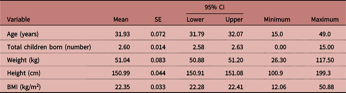
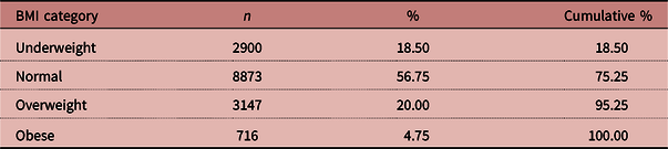
The age of the women ranged from 15 to 49 years, with a mean of 31.93±90.00 years (95% CI: 31.79–32.07). The average heights and weights of the women were 150.99±5.50 cm (95% CI: 150.91–151.08) and 51.04±10.37 kg (95% CI: 50.88–51.20), respectively. Their mean BMI was 22.35±4.12 kg/m2 (95% CI: 22.28–22.41) (Table 1). Over half (56.75%) had a BMI in the normal range (18<BMI<25 kg/m2), whereas 18.50%, 20.00% and 4.75% were underweight (BMI≤18 kg/m2), overweight (25≤BMI<30 kg/m2) and obese (BMI≥30 kg/m2), respectively (Table 2).
Descriptive statistics of non-pregnant women of reproductive age, BDHS-2014 (N=15,636)

Distribution of BMI levels of non-pregnant women of reproductive age, BDHS-2014

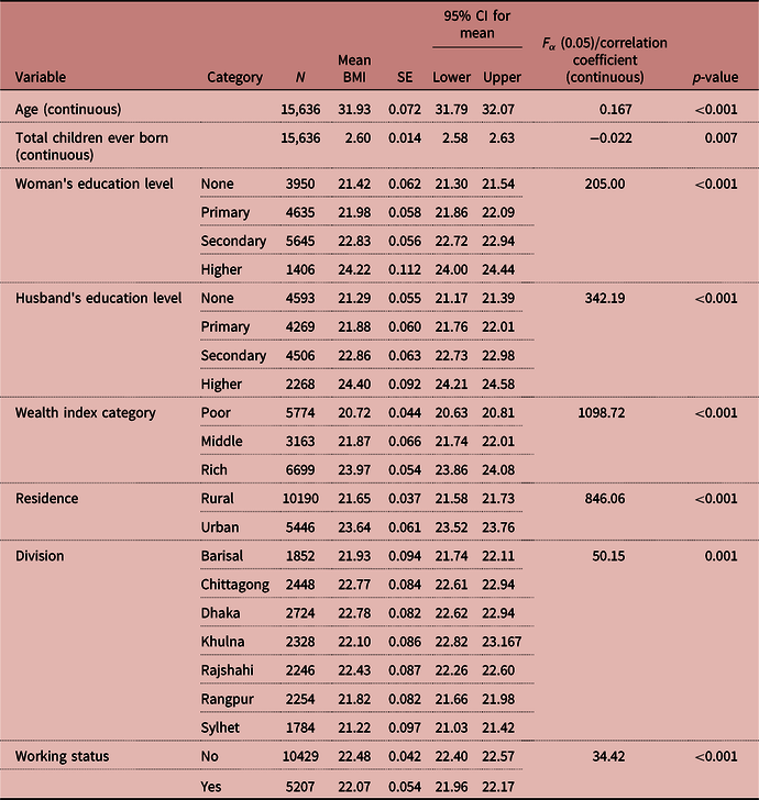
The ANOVA analyses found that womenʼs education level, husbandʼs education level, wealth index group, urban/rural place of residence, geographical division and working status were significantly associated (p<0.001) with the womenʼs mean BMI. The t-test demonstrated that the mean BMI was higher for women from rich and urban areas (p<0.001), those with higher education (p<0.001), those with a highly educated husband (p<0.001), those who were not working (p<0.001) and those residing in Dhaka city (p<0.001) compared with other groups (Table 3). Pearsonʼs correlation coefficient demonstrated that the correlation between BMI and age was positive (p<0.001). Womenʼs mean BMI and the total number of children ever born were found to be negatively associated (p=0.007) (Table 3).
Descriptive statistics of non-pregnant women of reproductive age by socio-demographic factors, BDHS-2014

Fα is the F-statistics having a cumulative probability of (1−α).
Results of Multiple Linear Regression analysis
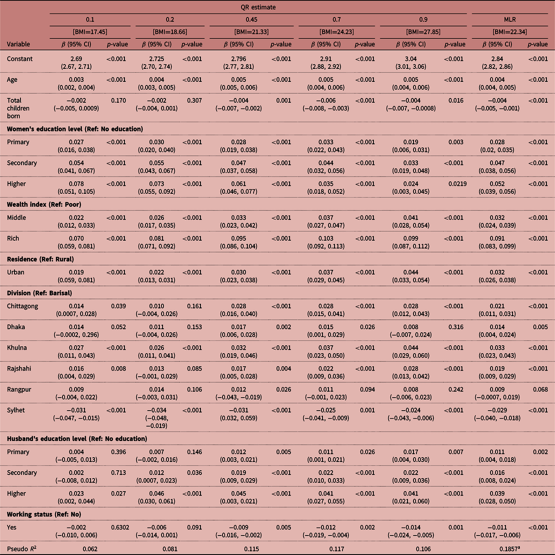
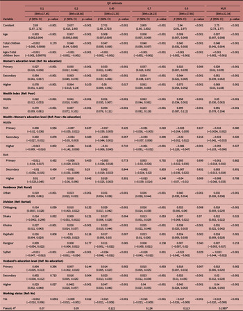
The MLR analyses showed that BMI was significantly associated with age, total children ever born, education level, husbandʼs education level, wealth index group, place of residence, geographical division and working status. Table 4 displays the results of the MLR as a baseline model and also the QR estimates at five selected quantile levels (0.1, 0.2, 0.45, 0.70, 0.9). These quantile levels were selected based on previous literature (Sharaf et al., Reference Sharaf, Mansour and Rashad2019).
Multiple Linear Regression (MLR) and Quantile Regression (QR) fitted to the socio-demographic factors with BMI

a R 2 for MLR.
The results from MLR showed that womenʼs age was positively associated (p<0.001) with BMI. The womenʼs BMI increased with increasing age by 0.46% per unit change of age. The total number of children ever born was negatively associated with BMI (p<0.001) and decreased by 0.35% per unit increase in the number of children.
Women from urban areas (p<0.001) and with a rich family background (p<0.001) had a significantly higher BMI than their counterparts. The BMI of urban women was 3.27% higher than that of rural women. The BMI of women from rich and middle-income families was 9.14% and 3.2% higher relative to poor families. Women with higher education (p<0.001) had a significantly higher BMI than those who were uneducated. The BMI of higher educated women was 5.26% higher than that of uneducated women, and 4.75% and 2.8% higher for the secondary and primary educated women, respectively.
Women with an educated husbands (primary, secondary, higher) had a significantly (p<0.001) higher BMI than those with uneducated husbands. It was 3.93%, 1.67% and 1.14% higher for higher, secondary and primary educated husbands compared with uneducated husband. Working women had a significantly lower BMI (1.18%, p<0.001) than those who were not working. Women residing in Sylhet had a lower BMI than those from other geographical divisions, and BMI was higher for the women residing in Khulna than those from other geographical divisions (p<0.001) (Table 4).
Results of Quantile Regression analysis
The QR analyses showed that womenʼs age was positively associated with their BMI (p<0.01) through the lower to upper quantiles of the BMI distribution. The percentage change in BMI distribution at quantile level 0.1 was 0.31% per unit change of age. The effect of age increased moving from the lower to the upper part of the BMI distribution. This indicates that higher BMI is associated with higher age. In this case, MLR overestimated the percentage change of BMI at lower quantiles and underestimated it at upper quantiles.
The effect of total number of children was not significant at the 0.1 and 0.2 quantile levels of the BMI distribution. The lack of significance in these two groups indicates that number of children was not associated with maternal BMI when BMI was low. However, the MLR did not display the change in estimates; it overestimated and underestimated at lower and upper quantiles, respectively.
Consistent with the results of MLR, the QR showed a positive association between womenʼs education level and BMI. The percentage change of the BMI distribution at the 0.1 quantile level was 7.86% higher for higher educated women compared with uneducated women. At each considered quantile, BMI was higher for higher educated women compared with secondary and primary educated women. This indicated that higher educated women tended to have higher BMIs. However, QR showed some discrepancies in the case of husbandʼs education. The BMI of women whose husband had only primary education showed an insignificant effect on BMI at the 0.1 and 0.2 quantile levels and a similar insignificance was observed at the 0.2 quantile level for secondary educated husbands.
Women from rich families had a higher BMI compared with those from poor and middle-income families. The effect size of wealth (Rich) increased on BMI from the lower to upper quantiles. At each considered quantile, the BMI of rich family women was higher than those from middle-income and poor families.
As for place of residence, the BMI of women living in urban areas increased at lower to upper quantiles. However, MLR underestimated the effect sizes (beta scores) at upper quantiles and overestimated them at lower quantiles. The working status effect gradually decreased from the lower to upper quantiles of BMI. This suggests an increase in working status with decreasing BMI. Working status was not significant at the 0.1 quantile level of the BMI distribution, because a lower BMI quantile level was not significantly associated with working status (Table 4).
The MLR estimate showed that geographical division had a significant effect on BMI. However, not all geographical divisions were equally associated with BMI. Some were not significant, and some were less statistically significant at different quantiles, which was not estimated by MLR. The QR provided more details on the association between BMI and geographical divisions (Table 4).
The Pseudo R θ 2 increased from lower to upper quantile levels (0.1, 0.2, 0.45, 0.7, and 0.9), suggesting that the effect of the associated variables increased on BMI from lower to upper quantiles, and it was advantageous to move from lower to higher quantiles. The R 2 value for the MLR model was 0.1857, which is much smaller, indicating a weak fit (Table 4). There are many variables that affect womenʼs BMI at reproductive ages but only some of the variables were included here. Some potential variables, such as weight objectives, weight-reduction techniques, body-shape discernments, eating attitudes and behaviours, self-idea and physical activity, level of energy intake and age at menarche (Kamruzzaman et al., Reference Kamruzzaman, Mamun, Bakar, Saw, Kamarul, Islam and Hossain2017) were not available in the data. This could be a potential reason for the smaller R 2 values in the MLR model.
Table 5 shows the results of MLR as a baseline model and also the QR estimates at five selected quantile levels (0.1, 0.2, 0.45, 0.70, 0.9) with interactions between age and total children born, and also the interaction between education and wealth index. The interaction between age and total children born was negatively associated. This means that increasing the level of age for a fixed number of children will decrease the BMI. Similarly, increasing the number of children for fixed ages will decrease the BMI. The QR showed that the effect of the interaction term ‘age and total children born’ was fixed at the considered quantiles (Table 5). The interaction between education and wealth was significant only for some combinations of education and wealth categories. The MLR showed that secondary and higher education with middle income had a significant positive effect on BMI. Education level with middle income showed a significant association at the 0.7 quantile level. Higher educated women with middle family income showed a significant association at the lower (0.1 quantile) and upper quantiles (0.9 quantile). The MLR showed that if secondary education was considered, then the effect difference (0.05+0.051–0.022=0.079) on BMI between middle and poor family women was 7.90% higher compared with no education. Similarly, if higher education was considered, then the effect difference (0.05+0.069–0.055=0.064) on BMI between middle and poor was 6.40% higher than no education. This means that increasing the education level decreased the effect difference on BMI between economic status. The results of the QR model showed that some of the combinations were significant at lower quantiles and others were significant at upper quantiles, which were not captured by MLR.
Multiple Linear Regression (MLR) and Quantile Regression models (QR) fitted to the socio-demographic factors with BMI (with interaction term)

a R 2 for MLR.
After adding the interaction term, the new R 2 value was 0.1989, which was an improvement compared with previous model in Table 4. The value of Pseudo R θ 2 also improved at each quantile (Table 5). This indicated a better fit compared with the previous model.
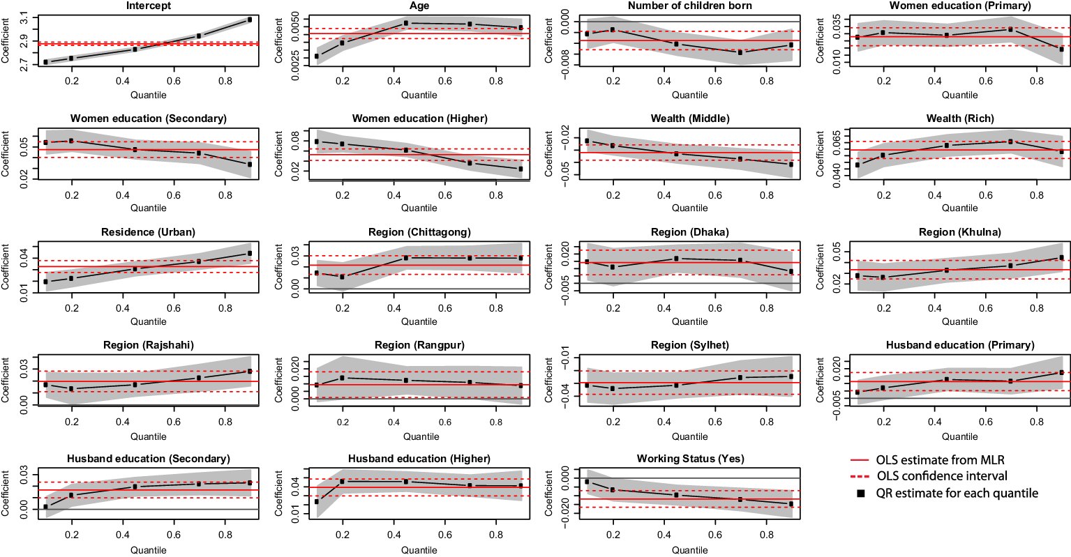
Figure 1 displays the MLR and QR estimates over the BMI determinants across the entire BMI distribution. The QR explained the heterogeneous response of BMI of women at reproductive ages for different socio-demographic factors at different tails of the BMI distribution. The figure shows that MLR overestimated (or underestimated) the effects of age, wealth index group, place of residence and husbandʼs education on BMI at lower (or higher) quantiles of the conditional BMI distribution. While MLR provided an average change across the BMI distribution, QR provided a complete interrelation between BMI and socio-demographic factors throughout the BMI distribution (Model 1).
Multiple Linear Regression (MLR) and Quantile Regression (QR) estimates for BMI determinants.

Discussion
This study attempted to detect the most vulnerable cohorts of reproductive age group women in Bangladesh at the two extremes of the BMI spectrum using MLR and QR models. Several factors were found to be significantly associated with these womenʼs BMI status. While more than half of the women (56.75%) were of normal weight, 18.50%, 20.00% and 4.75% were underweight, overweight and obese, respectively.
The percentage of underweight women in rural areas was relatively high (9.10%) compared with urban areas, and the opposite was true for obesity (NIPORT, 2014). These findings are consistent with the literature from Bangladesh (Khan & Kraemer, Reference Khan and Kraemer2009; Hossain et al., Reference Hossain, Bharati, Aik, Lestrel, Abeer and Kamarul2012; Kamruzzaman et al., Reference Kamruzzaman, Mamun, Bakar, Saw, Kamarul, Islam and Hossain2017). Aside from the change of BMI in urban and rural areas, it was also found that age of women, the total number of children ever born, level of education, husbandʼs level of education, wealth index, geographical division and working status were significantly associated with womenʼs BMI through OLS and QR analyses.
This study showed that increased age was associated with elevated BMI in non-pregnant women of reproductive age in Bangladesh. Studies evaluating BMI and socio-demographic factors have found that age is an important factor influencing the BMI of women (Shafique et al., Reference Shafique, Akhter, Stallkamp, de Pee, Panagides and Bloem2007; Khan & Kraemer, Reference Khan and Kraemer2009; Hossain et al., Reference Hossain, Bharati, Aik, Lestrel, Abeer and Kamarul2012; Kamruzzaman et al., Reference Kamruzzaman, Mamun, Bakar, Saw, Kamarul, Islam and Hossain2017). Women in rural Bangladesh generally do not receive adequate nutrients, either due to poverty or because of poorer feeding as a female child. However, during pregnancy, with the many maternal health care programmes now available in rural areas, rural women acquire knowledge on health care that could lead to them to increase in weight (Kamruzzaman et al., Reference Kamruzzaman, Mamun, Bakar, Saw, Kamarul, Islam and Hossain2017). Also, in urban areas or affluent parts of the country, the intake of processed food has increased, which could lead to weight gain among older women, who are less active than younger women (Kamal et al., Reference Kamal, Hassan and Alam2015).
The study found that womenʼs BMI decreased with an increase in the number of children per mother. Most women in Bangladesh, particularly in rural areas, do not receive adequate antenatal care, and most deliver their babies at home without skilled birth attendants (NIPORT, 2014). Young mothers delivering at home and with more than two children have been found to be at higher risk of underweight (Islam et al., Reference Islam, Islam, Bharati, Aik and Hossain2016). This increases the risk of various health problems/diseases (abnormal vaginal flora, abortion) and consequently affects womenʼs BMI (Baqui et al., Reference Baqui, Lee, Koffi, Khanam, Mitra, Dasgupta and Quaiyum2019; Nonyane et al., Reference Nonyane, Norton, Begum, Shah, Mitra, Darmstadt and Baqui2019). Added to this is the fact that mothers are less likely to care about their own health and fitness than that of their families, increasing the chances of women ending up at the extremes of the BMI scale.
The study also found a significant effect of the interaction between age and total number of children born on BMI, with this showing a negative impact on BMI. At fixed ages, women with more children would be more burdened with the responsibility of providing for all their family members – a strong tradition in rural areas in this part of Bangladesh. With increasing age some of them eventually ignore their own health (Kamruzzaman et al., Reference Kamruzzaman, Mamun, Bakar, Saw, Kamarul, Islam and Hossain2017).
Women working outside the home were found to have lower BMIs than those who did not work outside the home. Islam et al. (Reference Islam, Islam, Bharati, Aik and Hossain2016) found that young women working outside the home in Bangladesh were at higher risk of being underweight. This makes sense in the context of Bangladesh as rural women or poor women in urban areas who work tend to do laborious work rather than desk jobs. On the other hand, being an unemployed urban woman would increase the chance of being overweight as they are likely to stay at home and avoid manual labour (Sarma et al., Reference Sarma, Saquib, Hasan, Saquib, Rahman, Khan and Ahmed2016).
The education levels of women and their husbands were found to be significantly associated with BMI. Higher educated women seemed to have higher BMIs, which could be because these women are more likely to be in sedentary occupation involving less physically intensive exercise, such as development research work (Balarajan & Villamor, Reference Balarajan and Villamor2009). Occupational sitting time is high for educated people, which increases their risk of overweight and obesity (Mummery et al., Reference Mummery, Schofield, Steele, Eakin and Brown2005). On the other hand, less-educated individuals are more often involved in manual labour work (Kabeer et al., Reference Kabeer, Mahmud and Tasneem2011; Kumar et al., Reference Kumar, Hossain and Gope2015). Also, educated women have less time to prepare home-cooked meals so will, in general, use ready-made food, which is often more calorific (Schmidhuber & Shetty, Reference Schmidhuber and Shetty2005; Baker & Friel, Reference Baker and Friel2014). The present study found a significant association between education and work status (χ 2=270.78, df=3, p<0.001), which accentuates this point. Like womenʼs education, the educational level of husbands has also been shown to be associated with womenʼs BMI (Rahman & Nasrin, Reference Rahman and Nasrin2009; Rahman et al., Reference Rahman, Mondal, Islam, Ahmed, Karim and Alam2015). An educated husband is more conscious about womenʼs health than an uneducated one (Murakami et al., Reference Murakami, Ohkubo and Hashimoto2017). The present study also showed that the prevalence of underweight was higher among women with illiterate husbands than among those with educated ones.
Financial solvency seemed to be associated with the shift from underweight to overweight in Bangladesh. Most poor, uneducated women in the BDHS-2014 were underweight, whereas rich, educated women tended to be overweight. This indicates that women from wealthy families have a greater intake of nutrients, whereas those from poor families remain undernourished as they cannot afford food (Das et al., Reference Das, Fahim, Islam, Biswas, Mahfuz and Ahmed2019). Furthermore, wealthier families tend to consume more processed food, now becoming popular in urban Bangladesh, compared with their poorer counterparts, which is a change in the traditional dietary intake giving rise to general weight gain (Morgan & Sonnino, Reference Morgan and Sonnino2010; Rahman, Reference Rahman2013).
The study also found a significant joint effect of education and wealth on BMI. Education and wealth may have different associations with womenʼs BMI, but BMI typically increases with increasing education and wealth levels (Balarajan & Villamor, Reference Balarajan and Villamor2009; Rahman, Reference Rahman2013) and decreases with lower levels of education and wealth (Kabeer et al., Reference Kabeer, Mahmud and Tasneem2011; Kumar et al., Reference Kumar, Hossain and Gope2015; Das et al., Reference Das, Fahim, Islam, Biswas, Mahfuz and Ahmed2019). The QR model results in the current study showed that womenʼs BMI increased with increasing level of wealth. Womenʼs higher wealth index (rich and middle) and higher education had a joint significant effect at higher BMI quantiles (0.9) (Table 5), indicating a higher likelihood of overweight and obesity. This may have been because most rich and higher educated women were living in urban areas. Urbanization may be a cause of overweight and obesity (Popkin, Reference Popkin2014; Neiderud, Reference Neiderud2015). Furthermore, women from rich families with higher education showed no significant effect at lower quantiles, which could be because they can afford more nutritious food, are more health conscious and receive proper health care, and are thus less likely to be underweight (De Jersey et al., Reference De Jersey, Nicholson, Callaway and Daniels2013). Education and wealth were weak predictors at lower levels of BMI, which corresponds with the existing literature (Cardozo et al., Reference Cardozo, Dune, Neff, Brocks, Ekpo, Barnes and Marsh2013; De Jersey et al., Reference De Jersey, Nicholson, Callaway and Daniels2013). Here, the QR model showed a more detailed change in effect sizes compared with the overall effect estimate of the MLR model.
Urbanization has led to a fast-paced economy with a dense population leading to a change in food intake with a higher consumption of fats and carbohydrates (Popkin, Reference Popkin2014; Neiderud, Reference Neiderud2015). In the present setting of Bangladesh, fast-food restaurants and ‘super shops’ are gaining popularity in urban areas, filling in as spots for a recreational family gathering (Harun et al., Reference Harun and Ahmed2013; Ashraf et al., Reference Ashraf, Akhter and Noor2014). Furthermore, with extended urban relocation towards already overcrowded cities, expanded housing and developments (buildings, shopping malls etc.) have been built on open spaces, reducing space for physical activity (Reardon et al., Reference Reardon, Boughton and Tschirley2015; Neupane et al., Reference Neupane, Prakash and Doku2015; Melby et al., Reference Melby, Orozco, Ochoa, Muquinche, Padro and Munoz2017). Thus, indoor recreational activities, such as television viewing, computer use and video games, have increased, increasing sitting time (Goryakin & Suhrcke, Reference Goryakin and Suhrcke2014). These are possible reasons for the higher percentage of overweight people in urban than rural areas reported in this study (NIPORT, 2014).
It was found that BMI was significantly lower in Sylhet compared with Barisal, but higher for all other geographical divisions. This could be because Sylhet remains behind in both education and economic conditions (Islam et al., Reference Islam, Angeles and Mahbub2006; Kabir et al., Reference Kabir, Khanam, Agho, Mihrshahi, Dibley and Roy2012; Tareque et al., Reference Tareque, Begum and Saito2014; Mohsena et al., Reference Mohsena, Goto and Mascie-Taylor2015).
Although the study results are analogous to findings in the literature, most previous studies applied linear regression or logistics regression when modelling BMI. These estimation methods might not be a good fit if the association between BMI and different socio-demographic factors is heterogeneous at different quantiles of BMI distribution. To address these drawbacks, the study also investigated the disparities between BMI and associated socio-demographic factors through QR analyses.
Taking account of the heterogeneous effects of the associated factors at different quantiles of the BMI distribution gives a detailed picture of the vulnerable cohorts and consequently paves the way for a clearer intervention strategy. Given the diversity in Bangladesh, optimizing a universal policy for improving the health status of women in the country is not possible. Adaptable approaches and targeted intervention measures are in order. For instance, increasing awareness about BMI in poor families and in rural areas to reduce the prevalence of underweight women, sponsoring nutrition-rich food, intervention measures based on geographical divisional disparities, the setting up of proper medical facilities, especially in rural areas, taking the initiative to improve the knowledge of uneducated people about health care and nutrition, could help improve the health status of women. The QR might be a better model here as it could specify the distribution of vulnerable quantiles; for example, QR could identify which wealth status quantiles are more vulnerable and need immediate attention. This study found that women from poor families with a lower education level, rich families with higher education, urban and rural areas women (who are underweight and overweight), women from Sylhet and women of reproductive age with a higher number of children were vulnerable cohorts requiring greater attention.
There were some limitations to this study. First, it was confined to women of reproductive age (15–49 years) due to limitation in the data. A generalized interpretation should be made with cautiously. Second, it was not possible to adjust for cluster, strata or individual survey weights as missing and pregnant women were omitted. Third, beyond the socio-demographic factors analysed, other important factors such as sleep duration, sitting time, food consumption level, work duration and food prices could not be added to the model due to data limitation. Finally, the study had a cross-sectional design and causal inference was therefore limited. Future studies could consider longitudinal data for further investigation.
In conclusion, this study has shown that the prevalence of underweight among women of reproductive age remained high in rural areas of Bangladesh in 2014, and there had been an increase in overweight in urban areas. Womenʼs high BMI was found to be associated with husbandʼs level education, elevated family solvency, geographical divisional disparities, rapid urbanization, age and being employed. Women with higher education and whose husbands had higher education, from rich families and in urban areas tended to be overweight, and uneducated women with uneducated husband, from poor families and in rural areas were likely to be underweight. A lower BMI was observed in Sylhet, and higher BMI in Dhaka and Chittagong. Health strategies concentrating on undernutrition and overweight need to consider the disparities in BMI by different socio-demographic factors.
Acknowledgments
The authors thank the DHS for allowing free access to their data bank. They also thank Md. Mohsin (Institute of Statistical Research and Training, University of Dhaka, Bangladesh) for valuable guidance.
Funding
This research received no specific grant from any funding agency in the public, commercial, or not-for-profit sectors.
Conflict of Interest
The authors have no conflicts of interest to declare.
Ethical Approval
The Bangladesh DHS was approved by the ICF Macro Institutional Review Board and the National Research Ethics Committee of the Bangladesh Medical Research Council (BMRC). Written consent for the survey was given by participants before interviews. The secondary data sets analysed in the study are freely available on request from the DHS website at http://dhsprogram.com/data/available-datasets.com.