1. Introduction
Hairpin-like vortices have been identified as the dominant coherent flow structures in transitional and turbulent boundary layers and free shear layers (Fiedler Reference Fiedler1988; Robinson Reference Robinson1991; Wu Reference Wu2010). To better understand the characteristics of these flows, it is important to study the creation and growth mechanisms of the hairpin vortices and the resultant wavepackets containing multiples of these flow structures. A turbulent spot in isolation provides a suitable environment to study how a hairpin vortex forms in a shear layer and how the formation of one such flow structure may produce a local flow environment that promotes the creation of similar structures in sequence.
Turbulent spots are localized regions of turbulent flow within a laminar shear layer. A turbulent spot may be created by the selective amplification of disturbances in a boundary layer via the Tollmien–Schlichting instability mode, as in the first observations of turbulent spots by Emmons (Reference Emmons1951), or be triggered by, for example, localized roughness elements (e.g. Chong & Zhong Reference Chong and Zhong2003), electric discharges (e.g. Wygnanski, Sokolov & Friedman Reference Wygnanski, Sokolov and Friedman1976), or intermittent wall jets (e.g. Perry, Lim & Teh Reference Perry, Lim and Teh1981). Early experiments such as those by Schubauer & Klebanoff (Reference Schubauer and Klebanoff1956) and Wygnanski et al. (Reference Wygnanski, Sokolov and Friedman1976) showed that sufficiently downstream of the location where a turbulent spot is induced, the spot characteristics, defined by mean quantities such as the streamwise convection velocity and the streamwise and spanwise spreading rates, are independent of the disturbance creating the spot. In the absence of a strong streamwise pressure gradient, a turbulent spot produced by a disturbance in the inner region of the boundary layer is shaped like a downstream-pointing arrowhead, the leading and trailing edges of which convect at approximately 88 and 55 % of the local free-stream velocity, respectively (e.g. Gostelow, Melwani & Walker Reference Gostelow, Melwani and Walker1996). The leading edge of the spot typically appears as a turbulent region overhanging a laminar region near the wall, and the length of the overhanging region may be multiples of the local boundary-layer thickness (Wygnanski et al. Reference Wygnanski, Sokolov and Friedman1976). A calmed region where the local flow exhibits increased stability relative to the local undisturbed boundary layer is typically observed in the wake of the turbulent spot (Schubauer & Klebanoff Reference Schubauer and Klebanoff1956). Studies have shown that the size and shape of the spot, the leading- and trailing-edge celerities, and the size of the calmed region in the wake of the spot are highly sensitive to the streamwise pressure gradient (Sankaran & Antonia Reference Sankaran and Antonia1988; Katz, Seifert & Wygnanski Reference Katz, Seifert and Wygnanski1990; D’Ovidio, Harkins & Gostelow Reference D’Ovidio, Harkins and Gostelow2001a ,Reference D’Ovidio, Harkins and Gostelow b ) and free-stream turbulence intensity (Yaras Reference Yaras2006). Such studies have resulted in increasingly refined engineering models that predict spot production and growth rates for a variety of surface and free-stream conditions (Volino & Simon Reference Volino and Simon1995; Roberts & Yaras Reference Roberts and Yaras2005), and are used in design optimization of advanced technology, such as highly loaded axial blades in gas turbine engines (Gostelow et al. Reference Gostelow, Melwani and Walker1996). Further development of such models to improve the prediction accuracy for the location of transition onset and the length of the transition region requires a clearer understanding of the physical mechanisms responsible for the growth of turbulent spots.
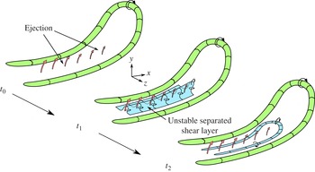
Schematic of the hairpin-vortex regeneration model proposed by Singer & Joslin (Reference Singer and Joslin1994).

Flow visualization experiments (e.g. Cantwell, Coles & Dimotakis Reference Cantwell, Coles and Dimotakis1978; Perry et al. Reference Perry, Lim and Teh1981), hot-wire and particle-image-velocimetry measurements (e.g. Makita & Nishizawa Reference Makita and Nishizawa2001; Schröder & Kompenhans Reference Schröder and Kompenhans2004; Chong & Zhong Reference Chong and Zhong2005; Yaras Reference Yaras2006; Schröder et al. Reference Schröder, Geisler, Elsinga, Scarano and Dierksheide2008), and direct numerical simulations (DNS) (e.g. Henningson, Spalart & Kim Reference Henningson, Spalart and Kim1987; Singer Reference Singer1996; Ovchinnikov, Choudhari & Piomelli Reference Ovchinnikov, Choudhari and Piomelli2008; Strand & Goldstein Reference Strand and Goldstein2011) have identified streamwise elongated hairpin vortices to be the dominant coherent flow structures in the turbulent spot. The shape and organization of the hairpin vortices within the spot resemble those found in turbulent boundary layers, although the distribution of vortices in the spot is typically more orderly (e.g. Schröder et al. Reference Schröder, Geisler, Elsinga, Scarano and Dierksheide2008). As the hairpin vortices extend in the wall-normal direction, they are stretched in the streamwise direction by the local wall-normal background shear. Hairpin vortices near the leading edge of the spot are stretched above a pocket of laminar flow near the wall and produce instantaneous inflectional velocity profiles in the laminar flow pocket, which destabilizes it to rapidly growing inviscid instability modes until this flow pocket is entrained into the turbulent spot (e.g. Henningson et al. Reference Henningson, Spalart and Kim1987), thus contributing to the streamwise growth of the spot. Vortex stretching also enhances the lateral growth of the spot, because conservation of angular momentum requires vorticity in the legs of the hairpin vortices to increase as the vortices stretch in the streamwise direction. This high level of vorticity induces wall-normal velocities towards and away from the wall (‘sweep’ and ‘ejection’, respectively) that create high- and low-speed streaks within the turbulent spot that are roughly aligned in the streamwise direction. Gad-El-Hak, Blackwelder & Riley (Reference Gad-El-Hak, Blackwelder and Riley1981) observed experimentally that the spanwise spacing of these streaks – typically approximately 100 wall units based on the average wall shear-stress within the turbulent spot – is approximately the same as in turbulent boundary layers (e.g. Cantwell et al. Reference Cantwell, Coles and Dimotakis1978; Perry et al. Reference Perry, Lim and Teh1981), and that the spanwise edge of the spot is consistently terminated by a low-speed streak. Henningson & Alfredsson (Reference Henningson and Alfredsson1987) confirmed through linear stability analysis that the streamwise velocity profile along the spanwise edges of the spot affected by a low-speed streak is less stable than the undisturbed local laminar flow.
Considering the important role of hairpin vortices in the growth of a turbulent spot, understanding the mechanisms by which these structures are created and grow within a spot is important. Through DNS, Singer & Joslin (Reference Singer and Joslin1994) studied the formation of hairpin vortices following the artificial triggering of a primary hairpin vortex. The regeneration mechanism of hairpin vortices observed in their results is shown schematically in figure 1. At time
 $t_{0}$
, the wall-normal velocities induced by the legs of the primary hairpin vortex eject low-momentum fluid away from the wall between the legs. Singer (Reference Singer1996) observed that the uplift of low-velocity fluid near the head of the primary vortex is weaker than near the legs, likely because the head of the primary hairpin vortex has experienced less streamwise stretching by the background shear than the legs and it resides in a region of lower background shear. Lift-up of the head of the primary vortex is a self-induced motion driven by the wall-normal velocities induced by the legs. By time
 $t_{1}$
, the ejected low-momentum fluid causes the fluid near the wall to separate from the surface. The vorticity of the separated fluid, which was originally oriented in the spanwise direction, is reoriented in the wall-normal direction to form an unstable separated shear layer. By time
 $t_{2}$
, the unstable separated shear layer rolls up into streamwise and spanwise oriented vortices to produce the legs and head of a secondary hairpin vortex. These mechanisms are qualitatively confirmed by visualization experiments of Guo et al. (Reference Guo, Lian, Li and Wang2004) and the vortex-regeneration model of Smith et al. (Reference Smith, Walker, Haidari and Sobrun1991) that is based on complementary experimental and computational studies of fully turbulent boundary layers.
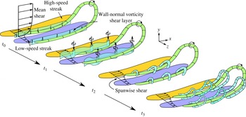
Recent tomographic particle-image-velocimetry measurements of triggered turbulent spots by Schröder & Kompenhans (Reference Schröder and Kompenhans2004) and Schröder et al. (Reference Schröder, Geisler, Elsinga, Scarano and Dierksheide2008) suggest an alternative regeneration mechanism of the hairpin vortices within the spot, illustrated in figure 2. Their results show that at time
 $t_{0}$
, strong spanwise shear is created between the high- and low-speed streamwise streaks, producing shear layers of wall-normal vorticity. By time
 $t_{1}$
, inviscid instability of this shear layer in the streamwise/spanwise (
 $x{-}z$
) plane leads to waviness in this plane that promotes streamwise grouping of wall-normal vorticity into coherent vortices oriented approximately in the wall-normal direction. By time
 $t_{2}$
, self-induced motions cause these vortices to fold over into arch-shaped structures that are then stretched in the streamwise direction to form secondary hairpin vortices by time
 $t_{3}$
. This mechanism is corroborated by the DNS performed by Krishnan & Sandham (Reference Krishnan and Sandham2007) of a spot triggered by a localized blowing trip, who observed that the lateral spot spreading rate is directly proportional to the magnitude of vorticity in the shear layer between the high- and low-speed streaks.
Schematic of the hairpin-vortex regeneration model proposed by Schröder and coworkers (Reference Schröder and Kompenhans2004, Reference Schröder, Geisler, Elsinga, Scarano and Dierksheide2008). For clarity, the high-speed streak that should appear on the
 $+z$
side of the primary hairpin vortex is omitted.

While the regeneration mechanism proposed by Singer & Joslin (Reference Singer and Joslin1994) implies that a secondary hairpin vortex will develop primarily between the legs of the primary hairpin vortex (figure 1), the mechanism proposed by Schröder and coworkers (Reference Schröder and Kompenhans2004, Reference Schröder, Geisler, Elsinga, Scarano and Dierksheide2008) implies that a secondary hairpin vortex will straddle a leg of the primary hairpin vortex (figure 2). Furthermore, due to the variable spanwise width of the streamwise streaks, the spacing between the wall-normal-vorticity shear layers at
 $t_{0}$
of figure 2 may vary. In cases when the wall-normal shear layers are in close proximity to each other, the wall-normal vortices at
 $t_{1}$
fold over towards the middle of the parent hairpin vortex and connect to each other, resulting in a secondary hairpin vortex forming between the legs of the parent hairpin vortex, resembling the topology described by Singer & Joslin (Reference Singer and Joslin1994). The published literature contains instances of turbulent spots with both kinds of hairpin-vortex topology, and it is not clear what flow conditions will favour one mechanism over the other. It is also not clear how either hairpin-vortex topology would relate to the mechanism(s) of lateral growth of the spot.
It is evident that a complete explanation for the growth mechanisms of flow structures within the spot has not yet been achieved. To contribute to this understanding, the present study investigates the development of a turbulent spot that is artificially triggered in a zero-pressure-gradient laminar boundary layer by a pulsed wall-normal jet. The results of this numerical study provide a complete history of the growth of the turbulent spot, thus providing insight into the growth mechanisms of the coherent flow structures within the spot and how these mechanisms relate to the lateral and longitudinal growth of the spot.
2. Numerical method
Accurately capturing the development of a turbulent spot in a numerical simulation requires spatial and temporal computational grids that are adequately refined to capture the spatial and temporal scales of the coherent flow structures within the spot, and a computational domain large enough to accommodate the unconstrained growth of the spot into a mature turbulent region. In the interests of computational efficiency, instead of a single simulation, two smaller DNS that are respectively optimized to capture the turbulent spot in its initial and later stages of development are performed to capture the full development history of the spot. Simulation 1 studies the initial formation of the coherent flow structures triggered in a zero-pressure-gradient laminar boundary layer by a pulsed transverse jet and their subsequent development into a young turbulent spot, while Simulation 2 studies the growth of this young turbulent spot into a mature turbulent region containing multiple instances of such vortical structures.
2.1. Computational domain
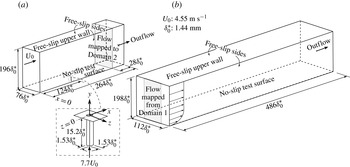
Simulations 1 and 2 are performed using Domains 1 and 2, respectively, shown in figure 3. Domain 1, shown in figure 3(a), consists of a flat, no-slip test surface with streamwise and spanwise dimensions of
 $264{\it\delta}_{0}^{\ast }$
and
 $76{\it\delta}_{0}^{\ast }$
, respectively, where the reference length scale,
 ${\it\delta}_{0}^{\ast }=1.44\ \text{mm}$
, is the displacement thickness of the undisturbed boundary layer in Domain 1 at the streamwise location where the turbulent spot is triggered. In both simulations, the working fluid is air at 1 atm and 25 °C. Triggering of the turbulent spot is accomplished by ejecting air from a rectangular jet sub-domain located at the midspan of the test surface and
 $124{\it\delta}_{0}^{\ast }$
downstream of the inlet plane. The origin of the coordinate system in Domains 1 and 2 coincides with the centre of the jet orifice. The side boundaries of the jet sub-domain are specified as no-slip walls with streamwise and spanwise dimensions of
 $1.53{\it\delta}_{0}^{\ast }$
and a length of
 $15.2{\it\delta}_{0}^{\ast }$
. Domain 2, shown in figure 3(b), has increased streamwise and spanwise dimensions of
 $486{\it\delta}_{0}^{\ast }$
and
 $112{\it\delta}_{0}^{\ast }$
, respectively, to allow for the continued growth of the spot without artificial influence by the domain boundaries. The spanwise width of both domains is such that the free-slip side walls are more than
 $30{\it\delta}_{0}^{\ast }$
away from the closest edge of the turbulent spot at its most mature state. Insensitivity to the spanwise domain width was confirmed by repeating Simulation 2 with the spanwise width increased by 50 % to
 $168{\it\delta}_{0}^{\ast }$
, with no change observed in the spanwise spreading rate of the spot. The wall-normal height of Domains 1 and 2 is chosen to allow the unconstrained development of the ejected jet above the test surface, as described by Brinkerhoff & Yaras (Reference Brinkerhoff and Yaras2012). To ensure a nominally zero streamwise pressure gradient along the test surface, the wall-normal height is adjusted in the streamwise direction following the displacement-thickness distribution of a Blasius boundary layer at the local flow Reynolds number.
Schematic of the computational domains. A magnified view of the jet sub-domain is shown framed by dashed lines. (a) Domain 1. (b) Domain 2.

2.2. Baseflow and turbulent spot initialization
A laminar boundary layer is developed on the test surface within Domain 1 by specifying a uniform inflow velocity and a uniform initial velocity field of
 $U_{0}=4.55\ \text{m}\ \text{s}^{-1}$
parallel to the test surface and computing to steady-state convergence. The no-slip condition on the test surface conflicts with the uniform velocity condition imposed at the inflow plane, resulting in a deviation between the computed velocity profile and the Blasius profile in close vicinity to this location. A streamwise distance of about
 $50{\it\delta}_{0}^{\ast }$
downstream of the inflow plane is required to recover the Blasius profile. The propagation of Tollmien–Schlichting (T–S) waves in the boundary layer requires a proper treatment of the compressibility of the working fluid, and because the present simulations solve the incompressible form of the governing equations (§ 2.4), they are not able to capture the natural development of T–S waves. This inability does not affect the development of the boundary layer because the local Reynolds number in Domain 1 remains below the critical Reynolds number, given by Schlichting (Reference Schlichting1968) as
 $\mathit{Re}_{crit}=U_{0}{\it\delta}^{\ast }/{\it\nu}=520$
. Furthermore, the inability to resolve T–S waves simplifies the examination of how the turbulent spot interacts with the background laminar boundary layer by removing the added effects of T–S waves. A laminar boundary layer is also developed on the test surface of Domain 2 by matching the flow conditions at the inflow boundary of Domain 2 to the undisturbed flow conditions at a spanwise/wall-normal plane located
 $28{\it\delta}_{0}^{\ast }$
streamwise distance upstream of the outflow boundary of Domain 1. A zero relative static pressure that is time-independent in an area-averaged sense is specified at the outflow boundary of the two domains. As a first-order discretization of spatial derivatives is used at the outflow boundaries, convective flow structures may be distorted as they exit the domain; the mapped plane in Domain 1 is located far enough upstream of the outflow boundary that the velocity field is not influenced by the presence of the outflow boundary.
Once a steady laminar boundary layer has developed in Domain 1, a turbulent spot is artificially triggered by impulsively applying a spatially uniform velocity of
 $7.7U_{0}$
magnitude at the inlet to the jet sub-domain for a duration of
 ${\it\tau}_{jet}=27$
time units, where
 ${\it\tau}=tU_{0}/{\it\delta}_{0}^{\ast }$
is the dimensionless time coordinate. The jet magnitude and duration were chosen to match a previous experimental investigation (Yaras Reference Yaras2006). The instant that the jet is deactivated corresponds to
 ${\it\tau}=0$
and Simulation 1 is continued until
 ${\it\tau}=303$
. Between
 ${\it\tau}=103$
and
 ${\it\tau}=303$
, the instantaneous velocity information in the spanwise/wall-normal plane
 $28{\it\delta}_{0}^{\ast }$
streamwise distance upstream of the outlet of Domain 1 is mapped to the inflow of Domain 2 as a transient inflow condition. The regions of Domain 2 on either side of the mapped data are specified with a steady, spanwise uniform velocity profile that corresponds to the local undisturbed laminar boundary layer as established
 $28{\it\delta}_{0}^{\ast }$
streamwise distance upstream of the outflow boundary in Domain 1. Insensitivity to the relative locations of the mapping plane and the outlet of Domain 1 was confirmed by repeating Simulation 1 with the outflow boundary moved
 $28{\it\delta}_{0}^{\ast }$
farther downstream. Within the mapped time interval, the triggered spot and the calmed region in its wake convect past the mapped plane and are introduced into Simulation 2 so that the complete history of the turbulent spot, from inception to maturity, is accurately captured in Simulations 1 and 2. The latest time when the wake of the spot is observable at the mapping plane in Simulation 1 occurs at
 ${\it\tau}=263$
. The full recovery from the presence of the spot is therefore conservatively assumed to occur by
 ${\it\tau}=303$
so that a steady, undisturbed laminar velocity profile can be imposed at the inflow of Simulation 2 for
 ${\it\tau}>303$
. Time integration is continued until
 ${\it\tau}=568$
. The transition-length correlation of Narasimha (Reference Narasimha1985) indicates that natural transition beginning at the moment the jet was triggered would take approximately 350 time units to complete under the free-stream conditions of the present study. This indicates that the turbulence observed in the spot for the majority of Simulation 2 corresponds to the turbulence that would be expected somewhat downstream of natural-transition completion, and thus the simulation duration is suitable to capture the full development of the spot.
2.3. Spatial grid
Structured grids consisting of hexahedral finite volumes are mapped to Domains 1 and 2. The spatial and temporal grids must be sufficiently refined to capture the smallest flow structures in the flow, which for turbulent flows are of the order of the Kolmogorov length and time scales. For wall-bounded turbulent shear layers, the Kolmogorov length scale is of the order of the viscous length scale, typically reaching a minimum value of
 ${\it\eta}^{+}\approx 2$
close to the no-slip boundary (Kim, Kline & Reynolds Reference Kim, Kline and Reynolds1971; Pope Reference Pope2000; Stanislas, Perret & Foucaut Reference Stanislas, Perret and Foucaut2008), where
 ${\it\eta}$
is the Kolmogorov length scale, the
 $+$
superscript denotes normalization with the viscous length scale,
 ${\it\nu}/u_{{\it\tau}}$
,
 $u_{{\it\tau}}=\sqrt{{\it\tau}_{w}/{\it\rho}}$
is the friction velocity,
 ${\it\tau}_{w}$
is the wall shear stress, and
 ${\it\nu}=1.53\times 10^{-5}\ \text{m}^{2}\ \text{s}^{-1}$
and
 ${\it\rho}=1.225\ \text{kg}\ \text{m}^{-3}$
are the kinematic viscosity and density of the working fluid, respectively. The friction velocity is calculated from the spatially averaged friction factor computed over the footprint of the spot at the final time step of Simulation 2. This friction velocity value agrees to within 1 % of the value based on the wall shear stress estimated from the local friction factor correlation for a fully developed turbulent boundary layer proposed by Schlichting (Reference Schlichting1968):
 $$\begin{eqnarray}C_{f}=(2\log _{10}(\mathit{Re}_{L})-0.65)^{-2.3}\end{eqnarray}$$
where
 $C_{f}=0.5{\it\tau}_{w}/{\it\rho}U_{0}^{2}$
is the local friction factor and
 $\mathit{Re}_{L}=309\,200$
is the Reynolds number based on
 $U_{0}$
and the effective streamwise length of the test surface,
 $L$
. The location of the spot at the last time step of the simulation from the inlet of Domain 1 dictates the value of
 $L$
; accounting for the mapping of flow information between Domain 1 and Domain 2, this length is
 $622{\it\delta}_{0}^{\ast }$
. Based on this value of the friction velocity, the nodes in Domains 1 and 2 are distributed to produce
 ${\rm\Delta}x^{+}=20$
and
 ${\rm\Delta}z^{+}=8$
in Domain 1 and
 ${\rm\Delta}x^{+}=20$
and
 ${\rm\Delta}z^{+}=7$
in Domain 2, corresponding to approximately 4–10 times the Kolmogorov length scale at the wall at the target Reynolds number. Similar spatial resolutions have been used by other researchers to study turbulent spots and turbulent boundary layers (e.g. Henningson et al.
Reference Henningson, Spalart and Kim1987; Spalart Reference Spalart1988). The present choice is validated in § 2.5. The spatial resolution of Domain 1 is refined in the vicinity of the jet orifice to about
 ${\rm\Delta}x^{+}\approx 8$
and
 ${\rm\Delta}z^{+}\approx 3$
to account for the smaller length scales in the initially triggered spot. The
 $y^{+}$
value of the nodes adjacent to the no-slip boundary within the spot is equal to or less than 0.7. In the range of
 $0.7<y^{+}<30$
, the wall-normal node spacing is increased linearly from the value adjacent to the wall to a value that corresponds to the Kolmogorov length scale in the log-law region, approximated by
 $$\begin{eqnarray}{\it\eta}^{+}=({\it\kappa}y^{+})^{\frac{1}{4}},\end{eqnarray}$$
where
 ${\it\kappa}=0.41$
is the von Kármán constant (Pope Reference Pope2000; Stanislas et al.
Reference Stanislas, Perret and Foucaut2008). Beyond
 $y^{+}=30$
, the node spacing is increased at a rate of 4 % until
 $y/{\it\delta}_{0}^{\ast }=5.0$
is reached. The grid spacing remains constant in the range of
 $5.0<y/{\it\delta}_{0}^{\ast }<8.7$
, with
 $y/{\it\delta}_{0}^{\ast }=8.7$
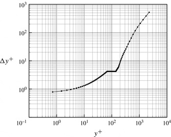
approximately corresponding to the height of the largest-scale flow structures expected in the triggered turbulent spot (e.g. Yaras Reference Yaras2006), and is then increased at a rate of 10 % until the free-slip ceiling of the domain is reached. This wall-normal node distribution is shown in figure 4.
Wall-normal node distribution.

The jet sub-domain is discretized with 60 nodes in each of the mutually perpendicular coordinate directions normal to the jet flow (
 $x$
and
 $z$
), spaced to place at least 20 nodes in the wall boundary layer of the jet, and the rate at which the node spacing varies in the
 $x$
and
 $z$
directions is less than 10 %. The direction parallel to the jet flow (
 $y$
) is discretized with 88 nodes that are distributed to place 15 nodes within
 $1{\it\delta}_{0}^{\ast }$
of the jet discharge plane. The
 $y$
direction nodes are clustered so that the spacing at the jet discharge plane is
 ${\rm\Delta}y^{+}=0.65$
and the spacing increases in the
 $-y$
direction at a rate of less than 10 % until
 ${\rm\Delta}y^{+}=4.0$
, after which the node spacing remains constant. The number of nodes in the streamwise (
 $x$
), spanwise (
 $z$
), and wall-normal (
 $y$
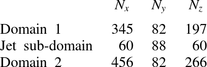
) directions in each computational domain are recorded in table 1.
Number of nodes in the spatial grid.

2.4. Solution method
ANSYS CFX® (Version 12), a commercial computational-fluid-dynamics software package, is used to solve the incompressible form of the time-varying mass and momentum equations through a finite-volume approach. This software package has been used extensively by the authors’ research group to simulate transitional and turbulent boundary layers, producing excellent agreement with experimentally measured parameters such as the velocity fluctuation spectra, turbulence-kinetic-energy production rate budgets, and mean velocity profile of turbulent boundary layers (McAuliffe & Yaras Reference McAuliffe and Yaras2010; Brinkerhoff & Yaras Reference Brinkerhoff and Yaras2011; Azih, Brinkerhoff & Yaras Reference Azih, Brinkerhoff and Yaras2012). Discretization of the governing equations is based on second-order central differencing and second-order Euler backward differencing for the spatial and temporal derivatives, respectively. In Simulation 1, a time step size of
 ${\rm\Delta}t=7\times 10^{-6}\ \text{s}$
is chosen so that the pulsed-jet flow takes approximately 10 time steps to penetrate a distance equivalent to the local displacement thickness of the undisturbed boundary layer at the jet discharge plane. In Simulation 2, a time step size of
 ${\rm\Delta}t=3.5\times 10^{-5}\ \text{s}$
or
 $0.11t^{+}$
is used, where
 $t^{+}={\it\nu}/u_{{\it\tau}}^{2}$
is the viscous time scale in the turbulent spot. Compared to the time step size of
 $0.20t^{+}$
recommended by Choi & Moin (Reference Choi and Moin1994) for accurately computing turbulent flows, the temporal resolution in the current study is quite conservative.
Solution convergence of the discretized equations at each time step is obtained with outer iteration loops serving to converge the coefficients of the linearized governing equations and inner iteration loops facilitating the solution of these equations through W-type algebraic multigrid cycles. Six grid levels are used in the multigrid cycle with one solution sweep performed at each grid level during the restriction passes and three solution sweeps performed at each grid level during the prolongation passes. The transient solution is obtained with one inner-loop iteration per outer-loop iteration, and multiple outer-loop iterations per time step. For each time step, the solution is declared as converged when the root-mean-square (r.m.s.) residuals of the governing equations are reduced by five orders of magnitude to less than
 $10^{-6}$
. This is realized with up to eight outer-loop iterations per time step. The simulations are partitioned and executed in parallel on 20 Intel™ L5410 Xeon processors.
2.5. Validation of numerical approach
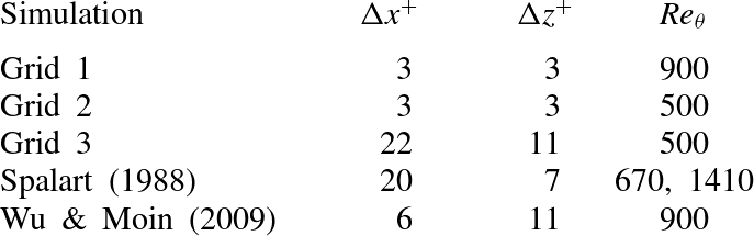
Validation of the numerical algorithm and the spatial and temporal resolutions was performed by Brinkerhoff & Yaras (Reference Brinkerhoff and Yaras2011) and Azih et al. (Reference Azih, Brinkerhoff and Yaras2012) through a series of companion DNS studies of a zero-pressure-gradient turbulent boundary layer and comparing the results of these validation simulations to statistical turbulence properties of corresponding turbulent boundary layers documented in the literature. The spatial grids and flow Reynolds numbers of these validation studies are listed in table 2. The dimensions of the computational domain for the simulations are 670, 1820, and 650 viscous units in the
 $x$
,
 $y$
, and
 $z$
directions, respectively, and the domain is spatially periodic in the streamwise and spanwise directions. The validation simulations are initialized with a spatially uniform velocity of
 $1.6\ \text{m}\ \text{s}^{-1}$
and the boundary layer is developed in time until a momentum-thickness Reynolds number of
 $\mathit{Re}_{{\it\theta}}=900$
is reached. Transition is triggered at
 $\mathit{Re}_{{\it\theta}}=450$
through a mass source/sink pair that is located near the wall in the centre of the domain. The trigger injects fluid into the domain at a wall-normal velocity of
 $0.16\ \text{m}\ \text{s}^{-1}$
for a duration of
 $4.5t^{+}$
.
Computational grids for the validation studies.

The first validation simulation (Grid 1) was performed at a Reynolds number based on the boundary-layer momentum thickness of
 $\mathit{Re}_{{\it\theta}}=900$
with a spatial resolution in the
 $x{-}z$
plane of
 ${\rm\Delta}x^{+}={\rm\Delta}z^{+}=3$
, which corresponds to approximately 1.5 times the Kolmogorov length scale at this Reynolds number. The
 $y^{+}$
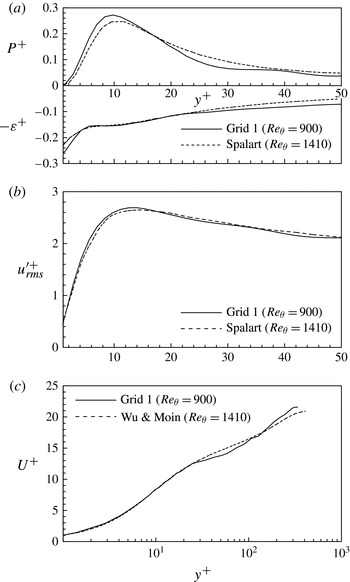
value of the first node from the no-slip boundary is 0.85 and the wall-normal node distribution (normalized using wall scales) follows closely the distribution shown in figure 4. Figure 5 shows that the results compare favourably to the turbulence kinetic energy production and dissipation rate budgets and the r.m.s. streamwise velocity fluctuation (
 $u_{rms}^{\prime +}$
) profiles (figure 5
a,b, respectively) computed by Spalart (Reference Spalart1988), who used an algorithm utilizing a spectral method for spatial discretization and a second-order accurate hybrid Runge–Kutta/Crank–Nicolson scheme for temporal discretization to simulate the boundary layer at a Reynolds number of
 $\mathit{Re}_{{\it\theta}}=1410$
. Figure 5(c) also shows excellent agreement in the mean velocity profile for
 $y^{+}<40$
when compared to the DNS results of Wu & Moin (Reference Wu and Moin2009) corresponding to
 $\mathit{Re}_{{\it\theta}}=900$
, who used a finite-difference scheme with second-order accuracy in space and mixed second- and third-order accuracy in time. Satisfactory agreement was also achieved in the outer part of the boundary layer, with a deviation of less than 10 % in the mean velocity profile. This deviation is due to the streamwise length of the computational domain used in the validation study being insufficient to fully capture the statistical properties of the larger-scale structures in the outer region of the turbulent boundary layer; this restriction does not apply in the present turbulent spot simulations, as the largest-scale structures within the turbulent spot are obviously confined to within the boundaries of the computational domain. The slight discontinuity in the mean velocity profile observed near
 $y^{+}=120$
is an artefact caused by an interface between sub-domains, as linear interpolation across the interface causes the spatial discretization to be locally first-order. This interface is not present in the turbulent spot simulations and no such artefact occurs.
Validation DNS study of a zero-pressure-gradient turbulent boundary layer at
 $\mathit{Re}_{{\it\theta}}=900$
. Results from Grid 1 are compared with (a) the turbulence kinetic energy production and dissipation rate distributions and (b) the streamwise velocity fluctuation profiles of Spalart (Reference Spalart1988), and (c) the mean velocity profile of Wu & Moin (Reference Wu and Moin2009). Adapted from Azih et al. (Reference Azih, Brinkerhoff and Yaras2012).

Validation DNS studies in a zero-pressure-gradient turbulent boundary layer at
 $\mathit{Re}_{{\it\theta}}=500$
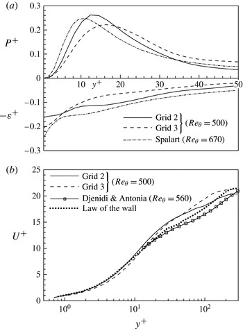
. Results from Grids 2 and 3 are compared with (a) the turbulence kinetic energy production and dissipation rate distributions of Spalart (Reference Spalart1988) and (b) the mean velocity profile of Djenidi & Antonia (Reference Djenidi and Antonia1993). Adapted from Brinkerhoff & Yaras (Reference Brinkerhoff and Yaras2011).

To isolate the effect of Reynolds number on the numerical results, a second validation DNS (Grid 2) was performed with the same spatial resolution as Grid 1 but at
 $\mathit{Re}_{{\it\theta}}=500$
, which is closer to the conditions of the present turbulent spot study, in which the Reynolds number based on the average momentum thickness in the spot at its most mature state is
 $\mathit{Re}_{{\it\theta}}=332$
. Finally, to ascertain the sensitivity of the results to the spatial grid, a third DNS (Grid 3), with a grid that closely matches the spatial resolution of the present turbulent spot study, was performed at
 $\mathit{Re}_{{\it\theta}}=500$
. The simulation results for Grids 2 and 3, shown in figure 6, compare reasonably well with the turbulence kinetic energy budgets computed by Spalart (Reference Spalart1988) at
 $\mathit{Re}_{{\it\theta}}=670$
and the mean velocity profile measured by Djenidi & Antonia (Reference Djenidi and Antonia1993) at
 $\mathit{Re}_{{\it\theta}}=560$
. Although the Grid 2 results are in slightly better agreement with the data of Spalart (Reference Spalart1988) and Djenidi & Antonia (Reference Djenidi and Antonia1993) than the Grid 3 results, the differences between the two cases and the benchmark data are similar to the ranges in the production and dissipation budgets observed by Honkan & Andreopoulos (Reference Honkan and Andreopoulos1997) among published experimental datasets at low Reynolds numbers. As such, the wall-normal node spacing and the spatial and temporal resolution of the present turbulent spot simulations are chosen to match those of Grid 3. This allows simulations with reasonable computing times while still ensuring that the flow physics are accurately captured. Considering that the transient coherent flow structures within a turbulent spot tend to be of greater spatial and temporal scales than in a fully turbulent boundary layer at comparable flow Reynolds numbers, the present study should accurately capture the flow development in the triggered turbulent spot. The suitability of the chosen spatial resolution is supported a posteriori by the observed agreement between the present simulation results and the published literature for the lateral spreading rate of the spot and the spatial characteristics of the low-momentum streaks within the spot, for example. To further ensure that the spatial resolution is sufficient, the spot initialization simulation (Simulation 1) was repeated using a spatial resolution equivalent to Grid 2. No observable changes occurred in the initial formation of flow structures within the young turbulent spot. While this does not directly attest to the adequacy of the computational grid at later times, it is reasonable to assume that the spatial resolution will continue to be sufficient when the spot is larger, as the dominant flow structures are correspondingly larger.
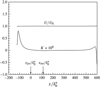
Streamwise distributions of the free-stream velocity,
 $U$
, and streamwise acceleration parameter,
 $K$
.

3. Results and discussion
3.1. Laminar baseflow
Figure 7 illustrates the free-stream conditions imposed on the laminar baseflow as it develops over the test surfaces of Simulations 1 and 2. The arrow in figure 7 at
 $x_{int}/{\it\delta}_{0}^{\ast }=112$
indicates the location where data are mapped between the two simulation domains. It is evident that the mapping has no effect on the free-stream flow development. Apart from short regions near the leading and trailing edges of the test surface, the free-stream acceleration parameter (
 $K={\it\nu}/U^{2}\partial U/\partial x$
) is close to zero, indicating that the laminar boundary layer develops in a way that closely resembles a zero-pressure-gradient boundary layer. The variations in
 $K$
near the leading and trailing edges correspond to peak variations of
 $U/U_{0}$
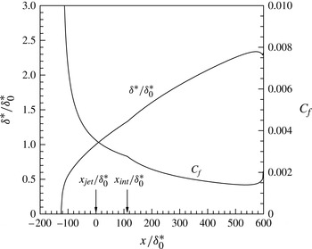
of less than 0.01. Figure 8 illustrates the streamwise distributions of the displacement thickness and friction factor of the undisturbed laminar boundary layer. These parameters show a small discontinuity at the location of the mapped plane,
 $x_{int}$
, indicating that the laminar boundary layer is slightly more sensitive to the mapping of flow information between simulation domains than the free-stream flow, but the magnitudes of the discontinuities in the streamwise gradients of
 ${\it\delta}^{\ast }$
and
 $C_{f}$
are very small, and unlikely to affect the development of the turbulent spot as it convects through the simulation domains. The maximum deviation between the computed values of
 ${\it\delta}^{\ast }$
and
 $C_{f}$
and the values given by the Blasius profile is 4 and 11 % of the local values, respectively, excluding the regions near the inflow and outflow boundaries. The change in the streamwise distribution slope of
 $K$
,
 ${\it\delta}^{\ast }$
, and
 $C_{f}$
that is observed near
 $x/{\it\delta}_{0}^{\ast }=600$
is due to the upstream influence of the outflow boundary. As such, the data beyond
 $x/{\it\delta}_{0}^{\ast }=500$
are discarded.
Streamwise distributions of the displacement thickness,
 ${\it\delta}^{\ast }/{\it\delta}_{0}^{\ast }$
, and friction factor,
 $C_{f}$
, of the undisturbed laminar boundary layer.

3.2. Formation of the turbulent spot
The growth of coherent flow structures within the triggered spot begins with the creation of vortices in the test-surface boundary layer by the triggering jet that resemble those occurring in the well-documented transverse-jet flow (e.g. Fric & Roshko Reference Fric and Roshko1994). A recent study by Brinkerhoff & Yaras (Reference Brinkerhoff and Yaras2012) showed that as the main-flow boundary layer convects around the jet, an adverse pressure gradient is created behind the jet that, when projected onto the test surface, causes the main-flow boundary layer to separate and roll into coherent streamwise oriented vortices immediately downstream of the jet orifice. These vortices are the ‘seed’ that initiates the formation of the turbulent spot.
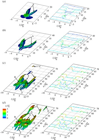
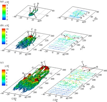
Formation of the turbulent spot in Simulation 1 illustrated at
 ${\it\tau}=2$
, 46, and 90, visualized through iso-contours of (a–c)
 ${\it\omega}_{x}=\pm 1$
and (d)
 $Q=0.6$
(left) and instantaneous vorticity lines (right). Iso-contours and vorticity lines are coloured according to the value of
 $y/{\it\delta}_{0}^{\ast }$
.

To illustrate the formation process, figure 9 plots iso-contours of perturbation streamwise vorticity,
 ${\it\omega}_{x}$
. The perturbation vorticity vector,
 ${\it\omega}_{i}$
, is defined as the curl of the perturbation velocity vector,
 $u_{i}$
, which in turn is defined as the local instantaneous velocity minus the velocity of the streamwise-local undisturbed laminar boundary layer at the same wall-normal location. Instantaneous lines of vorticity that intersect the vortices are also plotted to aid in visualizing the development of the vorticity field. The location of each vorticity line is carefully chosen so that it intersects the corresponding vortical structure at the same relative location at each time. The iso-contours are normalized by
 $(U_{0}/{\it\delta}_{0}^{\ast })^{2}$
and both the vorticity lines and iso-contours are coloured according to the value of
 $y/{\it\delta}_{0}^{\ast }$
to aid in comparing the relative heights of the vortical structures. At
 ${\it\tau}=2$
, the pair of streamwise oriented vortices created by the jet, labelled A, extend about
 $12{\it\delta}_{0}^{\ast }$
downstream of the jet orifice (located at
 $x/{\it\delta}_{0}^{\ast }=0$
,
 $z/{\it\delta}_{0}^{\ast }=0$
). The small-scale vortices above the jet orifice are remnants of vortices created by the triggering jet, which dissipate by
 ${\it\tau}=10$
. Because the A vortices are situated in the strain field associated with the laminar boundary layer, the vorticity field associated with the A vortices is stretched downstream so that by
 ${\it\tau}=46$
, the A vortices have elongated to roughly twice their length at
 ${\it\tau}=2$
. As a result, their peak magnitude increases to conserve angular momentum and thus the wall-normal motions induced by the A vortices become stronger and cause new generations of vortical structures to form. Figure 9(c) shows that by
 ${\it\tau}=90$
, two distinct pairs of secondary vortical structures – labelled B and C – occur near the A vortices and other tertiary vortical structures – labelled D, E and F – occur near the secondary vortical structures. To illustrate more clearly the shape of the secondary and tertiary hairpin vortices, figure 9(d) plots iso-contours of the second invariant of the velocity-gradient tensor, denoted
 $Q$
, defined as
 $$\begin{eqnarray}Q=\frac{1}{2}\left({\displaystyle \frac{\partial u_{i}}{\partial x_{j}}}^{2}-{\displaystyle \frac{\partial u_{i}}{\partial x_{j}}}{\displaystyle \frac{\partial u_{j}}{\partial x_{i}}}\right),\end{eqnarray}$$
where Einstein summation is implied over the indexed terms. This property has been shown to improve the prominence of the hairpin vortices over the background vorticity (e.g. Jeong & Hussain Reference Jeong and Hussain1995). The
 $Q$
iso-contours reveal that the B vortices are hairpin vortices that straddle the A vortices, the C vortices are streamwise vortices downstream of the A vortices, and the tertiary vortical structures (D, E, and F) are vortices formed by the B and C vortices. By
 ${\it\tau}=103$
(not shown), the A vortices have been stretched in the streamwise direction to about three times their length and twice their spanwise extent noted at
 ${\it\tau}=2$
.
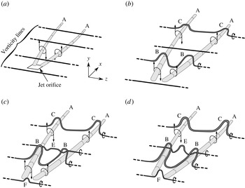
The process by which the multiple vortical structures observed in figure 9(d) form from the initial streamwise A vortices is discussed with the aid of the iso-contours and vorticity lines in figure 9 and a simplified schematic shown in figure 10. Because the turbulent spot is still in its infancy in figure 9, the process is not wholly representative of what occurs when the spot has reached maturity, and the detailed regeneration mechanism of vortical structures within the mature turbulent spot is discussed in § 3.4.1. Once the streamwise aligned A vortices are triggered by the transverse jet, they induce downwash in the region between the A vortices and upwash in the region outboard of the A vortices (figure 10
a). These wall-normal motions convect the local boundary-layer vorticity closer to and farther away from the wall, respectively, as illustrated in figure 9(a) by the vorticity lines labelled 2–5. As the A vortices are stretched in the downstream direction by the background strain field, the wall-normal motions they induce convect the boundary-layer vorticity outboard of the A vortices over and above the A vortices, as illustrated by the vorticity line labelled 6 in figure 9(c). The portion of vorticity line 6 that is situated above A is simultaneously convected towards the wall by the downwash between the A vortices so that the vorticity field associated with vorticity line 6 develops a significant wall-normal component. Inviscid instability of this layer of wall-normal vorticity causes it to roll up into a coherent B hairpin vortex (figure 10
b). A similar process occurs farther downstream to create the coherent C vortices. Figure 10(c) illustrates that as the B hairpin vortices are stretched by the background strain field, they elongate and are strengthened just like the A vortices. The downwash induced between the two B hairpin vortices convects the local boundary-layer vorticity towards the wall, as shown by vorticity line 5 in figure 9(d), to form the coherent E hairpin vortex, while the upwash induced upstream of the B hairpin vortices convects the boundary-layer vorticity away from the wall, as shown by vorticity line 7 in figure 9(d), and forms the coherent F hairpin vortex (figure 10
d). Stretching by the background shear increases the size and strength of the secondary and tertiary vortical structures. Between
 ${\it\tau}=103$
and 303, the spot is mapped into Simulation 2, where its continued streamwise and spanwise growth can be analysed in detail.
Schematic illustrating the formation of vortical structures in the early turbulent spot from the initial pair of streamwise vortices triggered by the transverse jet: (a)
 ${\it\tau}=2$
, (b)
 ${\it\tau}=46$
, (c)
 ${\it\tau}=68$
, (d)
 ${\it\tau}=90$
.

3.3. Defining the laminar/turbulent interface
Analysing the growth rate of a turbulent spot requires a consistent and precise method to identify the boundary between the laminar and turbulent flow regions. In a recent DNS by Strand & Goldstein (Reference Strand and Goldstein2011), the spanwise edges of the turbulent region were identified as the farthest locations on each side of the spot centreline where the magnitude of the streamwise component of vorticity
 $|{\it\omega}_{x}|$
exceeds a threshold value. This flow variable was used because it is nominally zero in undisturbed laminar flow regions and reaches high values in turbulent flow regions. At each time interval, spot-edge locations using several threshold values of
 $|{\it\omega}_{x}|$
were averaged to give one location on either side of the turbulent spot, which were subsequently averaged to obtain the spot half-width. This method yields the maximum half-width of the spot at a particular instant; the widest location typically occurs approximately 20–40 % of the spot length downstream of the spot’s trailing edge. This method was applied to the present numerical results with threshold values of
 $|{\it\omega}_{x}|{\it\delta}_{0}^{\ast }/U_{0}$
between 0.032 and 0.190 to produce the streamwise variation in the spot half-width, denoted
 $s$
, that is plotted in figure 11 with respect to the streamwise location of the spot’s trailing edge, denoted
 $x_{te}$
. To ascertain the sensitivity of the computed spot half-widths to the number of data points included in the averaging process, the method was repeated at selected instants in time using 4, 6, 8, 10, and 12 uniformly spaced threshold values between 0.032 and 0.190. The resulting uncertainty in the spot half-width, shown by the error bars in figure 11, indicates that identification of the spot edge with this technique becomes more precise as the spot matures. The abscissa in figure 11 is the streamwise location of the spot’s trailing edge, determined using the same threshold values of
 $|{\it\omega}_{x}|{\it\delta}_{0}^{\ast }/U_{0}$
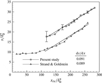
as those used for locating the spanwise edges of the spot. In comparison to the data of Strand & Goldstein (Reference Strand and Goldstein2011), reproduced in figure 11, the spot widths in the present study are consistently larger. Considering that the turbulent spot in the present study is triggered by a strong transverse jet, while the spot of Strand & Goldstein (Reference Strand and Goldstein2011) is triggered by a small roughness element, it is likely that the strong jet in the current study triggered a very rapid initial growth of the spot. Despite this offset, figure 11 shows that the spot lateral growth rates in the current study agree quite favourably with the results of Strand & Goldstein (Reference Strand and Goldstein2011). The average spot lateral growth ratio,
 $\text{d}s/\text{d}x$
, and the spot spreading half-angle, defined as
 $\tan ^{-1}(\text{d}s/\text{d}x)$
, are respectively 0.091 and 5.2° in the current study, compared to 0.089 and 5.1° found by Strand & Goldstein (Reference Strand and Goldstein2011). The trend observed in figure 11 suggests that the turbulent spot lateral growth ratio is constant starting at
 $x_{te}/{\it\delta}_{0}^{\ast }\approx 118$
, which corresponds to
 ${\it\tau}=255$
. The time range over which the spot lateral growth ratio can be assumed to have reached a constant value is thus
 ${\it\tau}=255{-}568$
. This period of spot growth is studied in detail in § 3.4 to analyse the steady growth mechanisms within the turbulent spot.
Streamwise distribution of the spot’s spanwise dimension.

Development of the turbulent spot at
 ${\it\tau}=107$
, 255, and 492, visualized through contours of
 $Q=0.6$
(left) and instantaneous vorticity lines (right) coloured according to the value of
 $y/{\it\delta}_{0}^{\ast }$
. The colour scale at
 ${\it\tau}=107$
is half of that at the other times.

3.4. Growth of the turbulent spot
Figure 12 illustrates the organization of vortical flow structures in the turbulent spot at
 ${\it\tau}=107$
, 255, and 492 by plotting
 $Q$
iso-contours at the same iso-contour level as in figure 9(d). Instantaneous vorticity lines are again shown, labelled according to the coherent vortical structures they intersect. As expected, the flow structures and vorticity lines have not changed appreciably between
 ${\it\tau}=90$
in figure 9 and
 ${\it\tau}=107$
in figure 12. Between
 ${\it\tau}=107$
and
 ${\it\tau}=255$
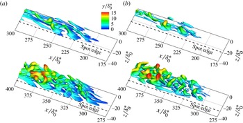
, however, the coherent vortical structures within the spot develop a pattern that remains fairly consistent for the rest of the lifetime of the spot. Figure 12(b,c) indicate that the pattern is as follows: numerous hairpin vortices of various spatial scales occur within the interior of the spot, such as those labelled B; larger-scale vortical structures occur near the leading edge of the spot, such as those labelled C, D, H, and G; and smaller-scale vortical structures occur near the trailing edge of the spot. Between
 ${\it\tau}=255$
and
 ${\it\tau}=492$
, the growth of the spot occurs as follows: new hairpin vortices are generated within the interior of the spot and form groups of two or three closely spaced hairpin vortices called ‘wavepackets’; the vortical structures near the leading edge of the spot are enlarged in their spatial scale; and new wavepackets of hairpin vortices are created at the laminar/turbulent interface along the spanwise edges of the spot. In the following sections, the detailed development of the spot is analysed in the context of these growth mechanisms. Additionally, the low population of hairpin vortices observed in figure 12(b,c) upstream of the trailing edge of the spot implies the development of a ‘calmed’ region in the wake of the spot; the development of this calmed region is discussed in § 3.4.4.
3.4.1. Regeneration of hairpin vortices within the interior of the spot
Figure 12 shows numerous hairpin vortices of various scales forming within the spot, among which a few distinct examples are highlighted to demonstrate the hairpin-vortex regeneration mechanisms occurring within the spot. The pair of hairpin vortices labelled C at
 ${\it\tau}=107$
join into a single hairpin vortex centred at approximately
 $z/{\it\delta}_{0}^{\ast }=0$
by
 ${\it\tau}=255$
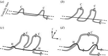
. The joining process is illustrated in figure 13 through a simplified schematic that is based on analysis of the simulation results at intermediate time steps. As the spot convects downstream, the pair of C hairpin vortices identified in figure 12 at
 ${\it\tau}=107$
are steadily lifted away from the wall through a self-induced lift-up effect (figure 13
b). On the basis of circulation conservation, the decreasing strength of the background strain rate away from the wall drives an increase in the lateral scale of the C vortices as they lift up (figure 13
c). The two C hairpin vortices grow increasingly closer to each other in the lateral direction and eventually join to form a single hairpin vortex by
 ${\it\tau}=255$
(figure 13
d). The vorticity in the legs of C induces strong upwash motions between the legs so that two new hairpin vortices are observed starting at
 ${\it\tau}=255$
, labelled H. The vorticity lines in figure 12 at
 ${\it\tau}=492$
indicate that the H hairpins straddle the legs of C.
Schematic illustrating the lateral joining of a pair of hairpin vortices into a single hairpin vortex: (a)
 ${\it\tau}=107$
, (b)
 ${\it\tau}=155$
, (c)
 ${\it\tau}=205$
, (d)
 ${\it\tau}=255$
.

Several smaller-scale hairpin vortices also develop within the interior of the spot near the hairpin vortices labelled B at
 ${\it\tau}=255$
. These smaller-scale hairpin vortices are organized into wavepackets consisting of multiple (typically two or three) closely spaced hairpin vortices that straddle one of the legs of the parent hairpin vortex, similar to the wavepackets observed in turbulent boundary layers (e.g. Adrian, Meinhart & Tomkins Reference Adrian, Meinhart and Tomkins2000). It is interesting to note that the wavepackets at
 ${\it\tau}=255$
do not occur throughout the spot but develop only near large hairpin vortices like B and C that extend far away from the wall. This suggests that in order for a wavepacket to form, the parent hairpin vortex must extend far enough into the free-stream fluid that it can be sufficiently stretched in the downstream direction. Under these conditions, the vorticity in the legs of the parent vortex increases to the point where it can induce strong upwash and downwash motions that in turn reorient the near-wall vorticity in the adjacent fluid to initiate the next generation of hairpin vortices.
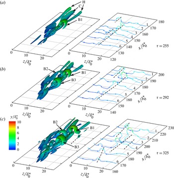
Magnified view of the development of a wavepacket between
 ${\it\tau}=255$
and 325, visualized through contours of
 $Q=0.6$
(left) and instantaneous vorticity lines (right). Iso-contours and vorticity lines are coloured according to the value of
 $y/{\it\delta}_{0}^{\ast }$
.

The streamwise growth of wavepackets occurs via the generation of multiple hairpin vortices from a single parent hairpin vortex. Figure 14 illustrates this process by plotting a magnified view of the wavepacket that occurs near the B hairpin vortex on the
 $+z$
side of the spot. An arbitrary number of vorticity lines coloured according to the value of
 $y/{\it\delta}_{0}^{\ast }$
are also plotted to better illustrate the vortex dynamics. The primary hairpin vortex at
 ${\it\tau}=255$
is labelled B1. The streamwise vortices that lie downstream of B1 correspond to the legs of the C and H hairpin vortices. The inboard leg of B1, indicated with a long dashed line, corresponds to the streamwise aligned sequence of perturbed vorticity lines labelled 2–6 in figure 14 at
 ${\it\tau}=255$
. Similarly, the perturbation in vorticity line 1 indicated by the short dashed line corresponds to the leg of the C hairpin vortex. By
 ${\it\tau}=292$
, this perturbation has lengthened longitudinally to include vorticity line 2 and has amplified so that a coherent vortex resembling the head of a hairpin vortex is observed in the iso-contours, labelled B2. By
 ${\it\tau}=325$
, B2 has grown farther from the wall into a clearly defined hairpin vortex. Returning to
 ${\it\tau}=255$
, a secondary perturbation of vorticity lines 3 and 4 is visible, indicated by the short dotted line. This secondary perturbation is created via a lift-up process whereby the stretching of the B1 vortex strengthens the vorticity field surrounding lines 3 and 4, which in turn induces the lift-up of the secondary perturbation, discussed further in § 3.5. As the amplitude of the primary B1 vortex grows with time, the strengthening of the vorticity field surrounding lines 3 and 4 continues, strengthening the lift-up process so that the wall-normal height of the secondary perturbation also amplifies with time. By
 ${\it\tau}=292$
, the perturbed vorticity field merges so that perturbed vorticity lines such as line 4 in close proximity to each other coalesce to produce a secondary hairpin, labelled B3, which is clearly visible in the iso-contours. By
 ${\it\tau}=325$
, B3 is nearly as tall as B1, and the stretching of B3 by the background shear amplifies the vorticity in its legs so that they begin to generate new perturbed vortex segments on the inboard side, as seen by the dashed line through vorticity lines 5 and 6, and on the outboard side, as seen by the dashed line through vorticity lines 3 and 4. Further time steps reveal that the perturbation of vorticity lines 5 and 6 grows to produce a new wavepacket with multiple new hairpin vortices.
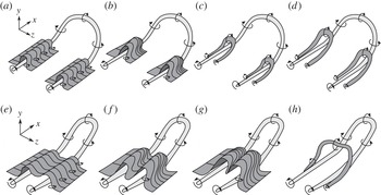
Schematic illustrating the regeneration of hairpin vortices from a parent hairpin vortex with (a–d) widely spaced and (e–h) closely spaced legs.

The regeneration process visible in figure 14 can be summarized using the simplified schematics presented in figure 15. The wall-normal motions induced by the legs of the parent hairpin vortex (B1 in figure 14) reorients the surrounding boundary-layer spanwise vorticity in the wall-normal direction (figure 15
a). The reoriented vorticity is stretched in the streamwise direction by the background shear and the shear layer formed by the wall-normal component of vorticity rolls up due to an inviscid instability in the
 $x{-}z$
plane, leading to streamwise grouping of wall-normal vorticity (figure 15
b). The roll-up forms one or more coherent secondary hairpin vortices that straddle a single leg of the parent hairpin vortex (figure 15
c) and subsequently grow due to self-induced lift-up and stretching by the background shear (figure 15
d). This process is similar to the mechanism proposed by Schröder & Kompenhans (Reference Schröder and Kompenhans2004) shown in figure 2. However, this is not the only hairpin-vortex regeneration mechanism observed in the present study. When the legs of the parent hairpin vortex are closely spaced in the
 $z$
direction, as sketched in figure 15(e), the regions of boundary-layer vorticity that are reoriented by the legs are also in close proximity to each other. As these regions of reoriented vorticity are stretched in the streamwise direction by the background shear, their spatial scales increase and they grow increasingly closer to each other (figure 15
f,g) until they eventually evolve into a single hairpin vortex that straddles both legs of the parent hairpin vortex (figure 15
h). The latter mechanism resembles the mechanism proposed by Singer & Joslin (Reference Singer and Joslin1994) and shown in figure 1. The mechanism depicted in figure 15(a–d) is observed most often in the present study among the larger-scale hairpin vortices near the leading and spanwise edges of the spot (such as vortices B in figure 12), while the mechanism depicted in figure 15(e–h) is observed only among the smaller-scale hairpin vortices that occur near the trailing-edge region of the spot. It should be stressed that despite the different outcomes for the widely and closely spaced parent hairpin vortices, it is the same fundamental physical process occurring in both.
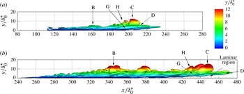
Turbulent spot at
 ${\it\tau}=255$
(a) and 492 (b), visualized through contours of
 $Q=0.6$
, viewed in the
 $-z$
direction.

3.4.2. Development of the leading-edge region of the spot
The hairpin-vortex regeneration process described in § 3.4.1 occurs at multiple locations within the interior of the turbulent spot so that by
 ${\it\tau}=492$
, multiple generations of wavepackets are present. Figure 12(c) shows that the population of wavepackets near the leading edge of the spot at
 ${\it\tau}=492$
is notably less dense than near the trailing edge. In contrast to structure B, structure C has not spawned a substantial number of smaller hairpins, and the streamwise elongated structures adjacent to it, labelled G, have not deformed into hairpin vortices. The side view of the spot seen in figure 16 shows that, especially at
 ${\it\tau}=492$
, structure C is located a notable distance away from the wall where the prevailing background strain rates are much lower than closer to the wall. The 99 % boundary-layer thickness of the undisturbed flow at
 $x/{\it\delta}_{0}^{\ast }=240$
is
 $4.42{\it\delta}_{0}^{\ast }$
, indicating that structure C reaches more than three times the local boundary-layer thickness above the wall. As a result, during this period of spot development, structure C undergoes a smaller degree of streamwise stretching than structures such as B that are located in closer vicinity to the wall. Furthermore, because the wall-normal gradients in the undisturbed streamwise velocity are greatly reduced (or are essentially non-existent) at this wall-normal distance, the background spanwise vorticity field – the deformation of which prompted the development of a series of new vortical structures around vortex B – would be absent for vortex C. Instead of spawning new hairpin vortices, figures 12 and 16 indicate that the vortical structures near the leading edge of the spot increase their spatial scale as the spot matures. This occurs due to the viscous diffusion of the vorticity from the vortical structures and the entrainment of low-speed fluid from the laminar region beneath the leading edge of the spot, as seen in figure 16, discussed in more detail below.
To quantify the longitudinal growth rate of the spot, the trailing- and leading-edge celerities are compared to the local velocities at the corresponding wall-normal locations in the undisturbed flow. As there is no standard practice for obtaining the undisturbed local velocity, denoted
 $U_{u}$
, it is estimated as
 $$\begin{eqnarray}U_{u}=\frac{1}{0.5y_{max}}\int _{0.25y_{max}}^{0.75y_{max}}U(y)\text{d}y,\end{eqnarray}$$
where
 $y_{max}$
is the maximum height of the coherent structures at the spot’s leading or trailing edge. The integration is performed at the trailing- and leading-edge locations for each streamwise station plotted in figure 11, and these values are respectively averaged to yield mean
 $U_{u}$
values of
 $0.50\pm 0.04U_{0}$
and
 $0.98\pm 0.02U_{0}$
at the trailing- and leading-edge locations, respectively; the uncertainties indicate the sensitivity to the integration bounds in (3.2) over a range of 0.1 to
 $1.0y_{max}$
. Relative to these values, the spot’s trailing and leading edges, which are identified in the manner described in § 3.3, move at an average speed of
 $0.04\pm 0.04U_{0}$
and
 $-0.14\pm 0.02U_{0}$
, respectively. Therefore, the corresponding leading- and trailing-edge celerities in the stationary frame of reference are
 $0.54U_{0}$
and
 $0.84U_{0}$
, respectively, which agree favourably with the celerities stated in the published literature for zero streamwise pressure gradient. These observations indicate that the streamwise movement of the spot’s trailing edge relative to the local undisturbed flow is essentially zero, while the leading edge of the spot moves at a slower rate than the local undisturbed flow.
The slower relative movement of the leading edge of the spot is caused by the entrainment of low-speed fluid from the laminar region. The mechanism for the entrainment of laminar fluid is observable in figures 12 and 16. As the C hairpin vortex grows within the spot, the downwash motion induced ahead of it by the spanwise oriented vorticity in its head is not spanwise uniform, and thus initiates a reorientation of the spanwise vorticity downstream of the C hairpin vortex, producing the streamwise vortices labelled D. Figure 16 shows that the streamwise D vortices are very prominent in the spot’s leading edge and are located much closer to the wall than the C hairpin vortex. As a result, their induced wall-normal motions are able to convect low-speed fluid into the spot’s leading edge (thus slowing down the leading edge relative to the local undisturbed flow) while also reorienting the spanwise vorticity in the laminar region into the wall-normal direction. The reoriented vorticity from the laminar region couples with the C or H hairpin vortices, which increases their overall circulation, as noted from the spatial scales of the H and C hairpin vortices in figure 16.
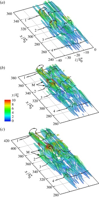
Growth of the turbulent spot at
 ${\it\tau}=480$
, 524 (a,b), and 568 (c), visualized through iso-contours of
 $|{\it\omega}_{y}|{\it\delta}_{0}^{\ast }/U_{0}=0.095$
shaded by
 $y/{\it\delta}_{0}^{\ast }$
in the
 $-z$
half of the spot. Solid lines illustrate vorticity lines that intersect the coherent vortical structures.

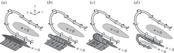
Schematic illustrating the regeneration mechanism of wavepackets along the spanwise edge of the turbulent spot.

3.4.3. Regeneration of wavepackets along the spanwise edges of the spot
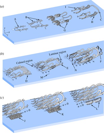
In figure 12, multiple wavepackets are observed along the spanwise edges of the spot near the location where the spot reaches its maximum width, which suggests that these wavepackets play a critical role in the lateral growth of the spot. To illustrate the process by which existing wavepackets within the spot generate new packets of hairpin vortices along the spot’s spanwise edge, figure 17 plots iso-contours of
 $|{\it\omega}_{y}|{\it\delta}_{0}^{\ast }/U_{0}=0.095$
in the
 $-z$
half of the spot. Vorticity lines that intersect the heads of hairpin vortices within the wavepackets are also plotted as an aid in connecting the coherent vortical flow structures to the surrounding vorticity field. The iso-contours are coloured according to the value of
 $y/{\it\delta}_{0}^{\ast }$
to show their relative heights and made semi-transparent to improve the visibility of the vorticity lines. The vortices that encompass the vorticity lines labelled 1 and 2 at
 ${\it\tau}=480$
correspond to hairpin vortices in the interior of the spot; the ‘head’ of the hairpin vortex consists of primarily
 $z$
-oriented vorticity and is thus not visible in the
 $|{\it\omega}_{y}|$
iso-contours. Vorticity line 1 is near the spot’s leading edge, and as such it undergoes minimal temporal variation for the reasons discussed in § 3.4.2. Vorticity line 2 is near the location of maximum spot width where the lateral growth rate of the spot is highest, and hence the vorticity field there undergoes a significant temporal evolution. At
 ${\it\tau}=524$
, the hairpin vortex encompassing line 2 has been stretched in the streamwise direction by the mean shear and the stretched vortex induces a wall-normal perturbation on the outboard segment of this vorticity line. The iso-surfaces in the region of the perturbed vorticity line, labelled M, indicate that two streamwise aligned regions of wall-normal vorticity are created, each one corresponding to the
 $-{\it\omega}_{y}$
and
 $+{\it\omega}_{y}$
regions indicated by the perturbed segments of vorticity line 2. By
 ${\it\tau}=568$
, the vorticity field surrounding lines 2 and 3 has been significantly perturbed in the wall-normal direction as the M-labelled regions of wall-normal vorticity have lengthened and become stronger.
The regeneration process visible in figure 17 can be summarized using the simplified schematics presented in figure 18. As in figure 15, the parent hairpin vortex induces upwash between its legs and downwash to the outside of its streamwise oriented legs. The upwash ejects low-momentum fluid and forms a low-speed streak between the legs of the parent hairpin vortex, while the downwash brings fluid with high streamwise momentum into the boundary layer on the outboard side of the parent vortex (figure 18 a). Because the hairpin vortex is located at the laminar/turbulent interface, the downwash of high-momentum fluid on its outboard side stretches the background spanwise vorticity into the streamwise direction, as shown in figure 18(a), introducing a streamwise component into the boundary-layer vorticity. The streamwise component of vorticity lifts up the stretched vorticity into the wall-normal direction (figure 18 b). As in figure 15, figure 18(c) shows that the wall-normal vorticity shear layers are unstable via an inviscid instability that produces streamwise grouping of wall-normal vorticity and the eventual roll-up of the wall-normal vorticity shear layers into one or more discrete hairpin vortices (figure 18 d). As the secondary hairpin vortex is stretched by the background shear, it becomes stronger and begins to induce wall-normal motions that form a new series of high- and low-speed streaks along the spanwise edge of the turbulent spot. This sequence indicates that the formation of new wavepackets along the spanwise edges of the spot follows the same fundamental processes as the creation of hairpin vortices within the spot interior described in § 3.4.1.
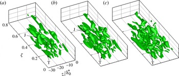
The regeneration of wavepackets along the spanwise edge of the spot can be linked to the temporal evolution of the velocity field at the same time instants shown in figure 17 by analysing the flow field at a constant streamwise location with respect to the spot’s trailing and leading edges. This is realized through a streamwise coordinate referenced to the spot’s trailing-edge location and normalized by the spot length, defined as
 $$\begin{eqnarray}{\it\zeta}=\frac{(x-x_{te})}{(x_{le}-x_{te})}\end{eqnarray}$$
where
 $x_{te}$
and
 $x_{le}$
are the streamwise locations of the trailing and leading edges of the spot, respectively. Figure 19 visualizes the streamwise streaks in
 $y{-}z$
planes at
 ${\it\zeta}=0.25$
, 0.50, and 0.75 through contours of
 $u/U_{0}$
, where
 $u$
is the perturbation velocity defined earlier. Three simulation times (
 ${\it\tau}=391$
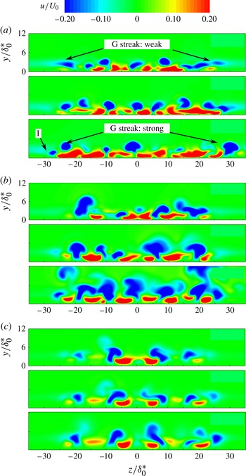
, 480, and 568) are shown to illustrate the development of the streamwise streaks as the spot develops. At all locations and times, the sides of the spot are consistently terminated by a low-speed streak. At
 ${\it\zeta}=0.25$
, shown in figure 19(a), the spanwise spacing of the interior streaks does not change significantly between the three simulation times, indicating that the spot’s lateral growth cannot be attributed to lateral spreading of the streaks as they are fed by the induced wall-normal motions of the hairpin and streamwise vortices, although their sizes do vary somewhat. The outermost streaks, which correspond to the structure labelled G in figure 12, are barely visible at
 ${\it\tau}=391$
, become stronger and larger at
 ${\it\tau}=480$
, and by
 ${\it\tau}=568$
have reached a size and strength that are comparable to those of the interior streaks. At
 ${\it\tau}=568$
, a new streak is observed on the
 $-z$
side of the spot, labelled I, suggesting that the creation of new wavepackets of hairpin vortices (and hence streaks) along the spanwise edges of the spot occurs with a temporal period close to
 $180{\it\tau}$
.
Contours of the streamwise perturbation velocity
 $u/U_{0}$
showing the development of streamwise streaks in the turbulent spot. Data are plotted in
 $y{-}z$
planes, located at (a)
 ${\it\zeta}=0.25$
, (b)
 ${\it\zeta}=0.50$
, and (c)
 ${\it\zeta}=0.75$
. The simulation times correspond to
 ${\it\tau}=391$
, 480, and 568.

3.4.4. Formation of the calmed region
A ubiquitous property of turbulent spots since the early observations of Schubauer & Klebanoff (Reference Schubauer and Klebanoff1956) has been the observation of a calmed region in the wake of the spot, upstream of the spot’s trailing edge, with a fuller streamwise velocity profile and thus enhanced stability prevailing in this region. Johnson (Reference Johnson2001) and Sabatino & Smith (Reference Sabatino and Smith2008) noted that the calmed region forms due to the wall-normal transfer of high-momentum fluid from higher in the boundary layer towards the wall. Johnson (Reference Johnson2001) attributed this wall-normal momentum exchange to a spanwise aligned vortex that lies on the laminar/turbulent interface at the spot’s trailing edge, while Sabatino & Smith (Reference Sabatino and Smith2008) attributed it to the sweep motions induced by the hairpin vortices that form near the trailing edge of the spot. As no spanwise aligned vortex is observed near the spot’s trailing edge in the present numerical results (e.g. figure 12), the mechanism proposed by Johnson (Reference Johnson2001) is not supported by the present results. Furthermore, noting that the farthest upstream sets of hairpin vortices are still at least 10 % of the spot length downstream of the spot’s trailing edge (e.g. figure 17) while the calmed region extends more than 20 % of the spot length upstream of the spot’s trailing edge, it seems unlikely that the small hairpin vortices create such strong wall-normal motions that they are able to stabilize the flow so far upstream, as Sabatino & Smith (Reference Sabatino and Smith2008) propose. The present results therefore suggest that a different mechanism may be responsible for the formation of the calmed region.
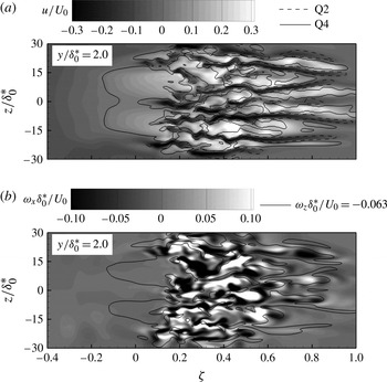
Formation of the calmed region upstream of the spot viewed through contours of (a)
 $u/U_{0}$
and (b)
 ${\it\omega}_{x}{\it\delta}_{0}^{\ast }/U_{0}$
in an
 $x{-}z$
plane at
 $y/{\it\delta}_{0}^{\ast }=2.0$
at
 ${\it\tau}=568$
. Lines in (a) are of Q2 (dashed) and Q4 (solid) and lines in (b) are of
 ${\it\omega}_{z}{\it\delta}_{0}^{\ast }/U_{0}=-0.063$
. The solid vertical line indicates the location of the spot’s trailing edge.

To illustrate this mechanism, figure 20 plots the instantaneous flow field in the wake of the spot at
 ${\it\tau}=568$
in an
 $x{-}z$
plane located at
 $y/{\it\delta}_{0}^{\ast }=2.0$
. Figure 20(a), which plots contours of the streamwise perturbation velocity, shows that the spot wake contains wide high-speed streaks in the boundary layer. These high-speed streaks account for the extra momentum that yields the fuller, more stable velocity profile within the calmed wake. The loci of upwash and downwash motions (Q2 and Q4, respectively) plotted in figure 20(a) show that while regions of upwash are predominately confined to within the spot, large regions of downwash are observed in the calmed wake and coincide with the locations of the wide high-speed streaks, indicating that the streaks are indeed created by wall-normal momentum transfer from the high-speed fluid farther from the wall, as proposed by Johnson (Reference Johnson2001) and Sabatino & Smith (Reference Sabatino and Smith2008), although apparently from a different origin than they propose. Figure 20(b) illustrates the origin of the downwash motions by plotting contours of streamwise perturbation vorticity,
 ${\it\omega}_{x}$
, and lines of spanwise perturbation vorticity,
 ${\it\omega}_{z}=-0.063U_{0}/{\it\delta}_{0}^{\ast }$
in the same
 $x{-}z$
plane as figure 20(a). The contour lines of
 ${\it\omega}_{z}=-0.063U_{0}/{\it\delta}_{0}^{\ast }$
show that the downwash is created by streamwise aligned sheets of enhanced spanwise vorticity that extend from the spot into the wake and coincide directly with the locations of the high-speed streaks observed within the wake. As the spot convects downstream, the fluctuating spanwise vorticity embedded in the slower-moving fluid near the wall extends from the spot’s trailing edge into the wake, inducing downwash motions and producing a calmed region that grows in sync with the longitudinal growth of the spot. Viscous diffusion limits the effective streamwise length of the strips of enhanced spanwise vorticity, ensuring that the calmed region has a finite length.
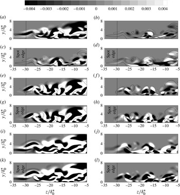
Contour levels of the budgets of the instantaneous vorticity transport equation (3.4) in the
 $-z$
side of the spot at
 ${\it\tau}=568$
and
 $x/{\it\delta}_{0}^{\ast }=345$
. Lines in (a–d) are
 $\widetilde{{\it\omega}}_{x}{\it\delta}_{0}^{\ast }/U_{0}=0.03$
(solid) and
 $-0.03$
(dashed). Lines in (e–h) are
 $\widetilde{{\it\omega}}_{y}{\it\delta}_{0}^{\ast }/U_{0}=0.03$
(solid) and
 $-0.03$
(dashed). (a)
 $\partial \tilde{{\it\omega}}_{x}/\partial t$
, (b)
 $\tilde{{\it\omega}}_{x}$
-stretching, (c)
 $\tilde{{\it\omega}}_{x}$
-transport, (d)
 $\tilde{{\it\omega}}_{x}$
-tilting, (e)
 $\partial \tilde{{\it\omega}}_{y}/\partial t$
, (f)
 $\tilde{{\it\omega}}_{y}$
-stretching, (g)
 $\tilde{{\it\omega}}_{y}$
-transport, (h)
 $\tilde{{\it\omega}}_{y}$
-tilting, (i)
 $\partial \tilde{{\it\omega}}_{z}/\partial t$
, (j)
 $\tilde{{\it\omega}}_{z}$
-stretching, (k)
 $\tilde{{\it\omega}}_{z}$
-transport, (l)
 $\tilde{{\it\omega}}_{z}$
-tilting.

3.5. Quantitative description of the spot growth mechanisms
A quantitative description of the physical mechanisms contributing to the development of new wavepackets along the spanwise edges of the turbulent spot, which was described qualitatively in § 3.4.3, is obtained by examining the inviscid transport equation for the instantaneous vorticity vector,
 $\widetilde{{\it\omega}}_{i}$
:
 $$\begin{eqnarray}{\displaystyle \frac{\partial \widetilde{{\it\omega}}_{i}}{\partial t}}=-\widetilde{u}_{j}{\displaystyle \frac{\partial \widetilde{{\it\omega}}_{i}}{\partial x_{j}}}+\widetilde{{\it\omega}}_{j}{\displaystyle \frac{\partial \widetilde{u}_{i}}{\partial x_{j}}},\end{eqnarray}$$
where
 $\widetilde{u}_{i}$
is the instantaneous velocity vector and Einstein summation is implied over the indexed terms. The terms on the right-hand side of (3.4) represent the convective transport of
 $\widetilde{{\it\omega}}_{i}$
and its production by vortex stretching and tilting, respectively. Figure 21 plots the distribution of the vector components of (3.4) normalized by
 $(U_{0}/{\it\delta}_{0}^{\ast })$
at time
 ${\it\tau}=568$
in a
 $y{-}z$
plane that intersects the spot at
 ${\it\zeta}=0.3$
. Production due to vortex stretching (
 $\widetilde{{\it\omega}}_{i}\partial \widetilde{u}_{i}/\partial x_{i}$
) and vortex tilting (
 $\widetilde{{\it\omega}}_{j}\partial \widetilde{u}_{i}/\partial x_{j},i\neq j$
) are plotted separately to distinguish the two processes. The vertical line at
 $z/{\it\delta}_{0}^{\ast }=29.7$
indicates the spanwise edge of the spot as identified in § 3.3. In figures 21(a–d) and 21(e–h), contour lines of
 $\widetilde{{\it\omega}}_{x}{\it\delta}_{0}^{\ast }/U_{0}=\pm 0.03$
and
 $\widetilde{{\it\omega}}_{y}{\it\delta}_{0}^{\ast }/U_{0}=\pm 0.03$
are respectively drawn to link the vorticity transport processes to the local vorticity distributions. Temporal variation of vorticity outboard of the spot is observed to occur predominantly in the
 $\widetilde{{\it\omega}}_{x}$
and
 $\widetilde{{\it\omega}}_{z}$
components, seen in figure 21(a,i), respectively, while the rate of change of
 $\widetilde{{\it\omega}}_{y}$
is much lower. The
 $\partial \widetilde{{\it\omega}}_{z}/\partial t$
contours in figure 21(i) correlate very strongly with the convective transport contours shown in figure 21(k). Such a correlation may suggest that the temporal variation of
 $\widetilde{{\it\omega}}_{z}$
outboard of the spot is primarily due to the transport of background vorticity by velocity fluctuations induced from existing vortical structures within the spot rather than the formation of new spanwise oriented vortical structures outboard of the spot. In contrast, the
 $\partial \widetilde{{\it\omega}}_{x}/\partial t$
contours appear to correlate with the production due to tilting of
 $\widetilde{{\it\omega}}_{x}$
shown in figure 21(d), while the stretching of existing
 $\widetilde{{\it\omega}}_{x}$
appears to have a minimal contribution to
 $\partial \widetilde{{\it\omega}}_{x}/\partial t$
. The
 $\widetilde{{\it\omega}}_{x}$
-tilting term also correlates well with the
 $\widetilde{{\it\omega}}_{x}$
contour lines that extend beyond the edge of the spot. These observations suggest that the positive growth rate of
 $\widetilde{{\it\omega}}_{x}$
outboard of the spot occurs primarily by the tilting of the laminar-boundary-layer vorticity outboard of the spot into the streamwise direction to form new, streamwise oriented coherent structures.
Linking the
 $\widetilde{{\it\omega}}_{x}$
-tilting term plotted in figure 21(d) to specific coherent structures developing outboard of the spot edge is facilitated by expanding it in terms of the instantaneous strain rates (e.g. Schoppa & Hussain Reference Schoppa, Hussain and Panton1997):
 $$\begin{eqnarray}\widetilde{{\it\omega}}_{j}{\displaystyle \frac{\partial \widetilde{u}_{i}}{\partial x_{j}}},i\neq j\equiv \left({\displaystyle \frac{\partial \widetilde{v}}{\partial x}}{\displaystyle \frac{\partial \widetilde{u}}{\partial z}}\right)-\left({\displaystyle \frac{\partial \widetilde{w}}{\partial x}}{\displaystyle \frac{\partial \widetilde{u}}{\partial y}}\right).\end{eqnarray}$$
The
 $\partial \widetilde{u}/\partial y$
strain rate is primarily formed by the background shear of the laminar baseflow, while the remaining instantaneous strain rates are formed by the coherent structures within the spot. This is illustrated in figure 22 by plotting the vorticity and velocity fields in the same
 $y{-}z$
plane as figure 21. The lines in figure 22(a) are the projection of the instantaneous vorticity field onto the
 $y{-}z$
plane and the contours illustrate the instantaneous streamwise vorticity,
 $\widetilde{{\it\omega}}_{x}{\it\delta}_{0}^{\ast }/U_{0}$
. The vectors shown in figure 22(b) are the instantaneous tangential (
 $\widetilde{v}/U_{0}$
and
 $\widetilde{w}/U_{0}$
) velocities and the contours illustrate the perturbation streamwise velocity,
 $u/U_{0}$
. The vorticity lines labelled 1–4 in figure 22(a) intersect a hairpin vortex that is situated near the edge of the spot; this is the same hairpin vortex that was shown previously in figure 17 encompassing vorticity line 2. The ejection of low-speed fluid between the legs of the hairpin vortex encompassing the vorticity lines labelled 1–4 generates the low-speed streak labelled G in figure 22(b) and hence a large local
 $\partial \widetilde{u}/\partial z$
strain rate is produced. The strain rate tilts the near-wall spanwise vorticity into the streamwise direction to produce the streamwise vortex labelled L. The L vortex induces strong sweep and ejection motions on its inboard and outboard sides, respectively, and hence a large local
 $\partial \widetilde{v}/\partial z$
strain rate is produced. The sweep motion produces the broad high-speed streak seen below the G streak in figure 22(b), while the ejection motion produces a low-speed streak, labelled I. Figure 22(b) also shows that due to the non-zero spanwise velocity component of the ejected fluid, a
 $\partial \widetilde{w}/\partial z$
strain rate is formed as the ejected fluid introduces spanwise motions outboard of the spot directed away from the spot. The near-wall spanwise motions noted outboard of the spot also contribute to the local
 $\partial \widetilde{w}/\partial z$
strain rate. These motions are created as the low-momentum fluid convects towards the spot to replace the near-wall fluid ejected by the L vortex.
Vorticity and velocity fields in the
 $-z$
side of the spot at
 ${\it\tau}=568$
and
 $x/{\it\delta}_{0}^{\ast }=345$
. In (a), lines are instantaneous vorticity lines projected onto the
 $y{-}z$
plane and contour levels are instantaneous streamwise vorticity. In (b), vectors are instantaneous velocity in the
 $y{-}z$
plane and contour levels are streamwise velocity perturbation.

Iso-contours of normalized (a)
 $\partial \widetilde{w}/\partial x$
(
 $(\partial \widetilde{w}/{\it\delta}x){\it\delta}_{0}^{\ast }/U_{0}=0.0025$
) and (b)
 $\partial \widetilde{v}/\partial x$
(
 $(\partial \widetilde{v}/{\it\delta}x){\it\delta}_{0}^{\ast }/U_{0}=0.0025$
) strain rates in the
 $-z$
side of the spot at
 ${\it\tau}=391$
and 568. Iso-contours are coloured by
 $y/{\it\delta}_{0}^{\ast }$
and the dashed line indicates the spanwise edge of the spot.

While figure 22 illustrates how the
 $\partial \widetilde{u_{i}}/\partial z$
strain rates are linked to the coherent structures present along the spanwise edge of the spot, it does not explain how the
 $\partial \widetilde{v}/\partial x$
and
 $\partial \widetilde{w}/\partial x$
strain rates in (3.5) are formed. The presence of these strain rates is illustrated in figure 23 by plotting normalized iso-contours of
 $\partial \widetilde{v}/\partial x$
and
 $\partial \widetilde{w}/\partial x$
on the
 $-z$
side of the spot at
 ${\it\tau}=391$
and 568. It is noted that as the spot matures, discrete regions of
 $\partial \widetilde{v}/\partial x$
and
 $\partial \widetilde{w}/\partial x$
strain rates are produced locally surrounding the hairpin vortices that are present along the spanwise edge of the spot. It is sufficient to note that because the parent hairpin vortices are of a finite length scale, the
 $\partial \widetilde{u_{i}}/\partial z$
strain rates they induce will be non-uniform in the streamwise direction, and hence the
 $\partial \widetilde{v}/\partial x$
and
 $\partial \widetilde{w}/\partial x$
strain rates will be non-zero. Furthermore, the finite length scale of new hairpin vortices generated along the spanwise edge of the spot is ensured due to the nature of the wavepacket regeneration process. As previously described in § 3.4.3 and illustrated in figure 18, once streamwise vorticity is formed along the outboard side of a parent hairpin vortex (such as vortex L in figure 22), the lift-up effect reorients the streamwise vorticity into the wall-normal direction, and the subsequent inviscid instability and roll-up of the wall-normal vorticity shear layers produces a discrete hairpin vortex. The shear-layer instability has a preferred streamwise wavelength and so ensures that discrete structures are produced. The resulting
 $\partial \widetilde{v}/\partial x$
and
 $\partial \widetilde{w}/\partial x$
strain rates contribute to the tilting-production of
 $\widetilde{{\it\omega}}_{x}$
outboard of the spot and thus participate in the wavepacket regeneration mechanism that drives the spanwise growth of the spot.
Iso-contours of normalized turbulence kinetic energy production,
 $P^{+}=0.5$
, at
 ${\it\tau}=480$
, 524 (a,b), and 568 (c) in the
 $-z$
half of the spot.

To visualize the contribution of the wavepacket regeneration mechanism to the turbulence kinetic energy of the fluid in the spot, iso-contours of the turbulence kinetic energy production rate, denoted
 $P_{k}^{+}$
, are plotted in figure 24. The production rate is normalized by
 $u_{{\it\tau}}^{4}/{\it\nu}$
. The plotted iso-contour level of
 $P_{k}^{+}=0.5$
is about half of the maximum value observed within the spot and was chosen on the basis that it likely shows the contribution of the most-energetic structures within the spot. The region labelled J corresponds to the hairpin vortex encompassing the projections of vorticity lines labelled 1–4 in figure 22. The turbulence kinetic energy production due to this structure changes only slightly from
 ${\it\tau}=480$
to 524, suggesting that it is a mature coherent structure and its contribution to the turbulence does not vary significantly in time until
 ${\it\tau}=568$
, at which time figure 24 shows that turbulence production moves to smaller scales. The region labelled T corresponds to the smaller-scale vortical structures that intersect the vorticity line labelled 4 in figure 17. The regeneration mechanism illustrated in figure 18 is activated by
 $\widetilde{{\it\omega}}_{x}$
in these regions, as seen in figure 17, and results in turbulence production that is relatively uniform at
 ${\it\tau}=480$
and aligned with the regions of strong
 ${\it\omega}_{y}$
shown in figure 17. As the regeneration mechanisms amplify, the production shifts to smaller scales, seen at
 ${\it\tau}=524$
. At
 ${\it\tau}=568$
, the young hairpin vortices that form from the wavepacket regeneration mechanism activated near structure T have enlarged to become regions of notable turbulence production. It is likely that if the simulation were continued further in time, these structures would continue to grow and stretch downstream until the production iso-contours resemble those of structure J. Figure 24 suggests that the formation and growth of the streamwise aligned
 $\widetilde{{\it\omega}}_{x}$
shear layers are a major factor in the growth of regions of high turbulence kinetic energy production due to their role in activating the regeneration mechanism of figure 18 to form new coherent structures, and hence have a significant impact on the growth of the turbulent spot.
4. Summary and conclusions
The growth of coherent flow structures in an artificially triggered turbulent spot is studied using two complementary direct numerical simulations. The first simulation captures the initial formation of hairpin vortices triggered by a pulsed jet and their development into a young turbulent spot, and a subsequent simulation captures the growth of the young turbulent spot into a mature turbulent region containing a large number of hairpin vortices. Mapping of transient flow information from the first to the second simulation domain allows for the full history of the turbulent spot to be accurately simulated, from creation to maturity. A schematic depicting the growth mechanisms occurring within the spot is presented in figure 25, and is used to summarize the findings of the present study.
Conceptual schematic summarizing the spot-growth mechanisms identified in the present study. (a) Initial growth after the spot is triggered. (b) Mechanisms leading to longitudinal growth of the spot. (c) Mechanisms leading to lateral growth of the spot.

The formation of coherent flow structures within the triggered spot begins as the triggering jet interacts with the test-surface boundary layer to form a pair of coherent, counter-rotating streamwise vortices within the boundary layer immediately downstream of the jet orifice (A). These vortices activate a hairpin-vortex regeneration process that produces new sets of hairpin vortices straddling the streamwise vortices (B). As the regeneration of new hairpin vortices continues, they form into wavepackets consisting of two to three closely spaced, streamwise aligned hairpin vortices. Spanwise merging of adjacent hairpin vortices also occurs, leading to an increase in their spatial scale (C).
New wavepackets are repeatedly generated along the spanwise edges of the spot, resulting in lateral growth of the spot at a rate that is in excellent agreement with the published literature. More wavepackets are observed near the trailing edge of the spot than at the leading edge, attributed to the fact that the hairpin vortices near the leading edge have much larger spatial scales and hence extend farther from the wall. As a result, the wall-normal motions induced by these large-scale hairpin vortices cannot form streamwise streaks and thus cannot activate the hairpin-vortex regeneration process. Instead, the spanwise non-uniform downwash motions induced by the large-scale hairpin vortices near the spot’s leading edge reorient the downstream spanwise vorticity (D) to form streamwise vortices that extend above the laminar overhang region below the spot’s leading edge (E). The wall-normal motions induced by these streamwise vortices convect fluid from the laminar region into the leading edge of the spot and reorient spanwise vorticity in the laminar region such that it strengthens the coherent vortical structures present near the leading edge (F), affecting an increase in their spatial scale. The convection and reorientation of vorticity accomplished by the leading-edge streamwise vortices result in the longitudinal growth of the spot at a rate that is in excellent agreement with the published literature.
The lateral growth of the turbulent spot is found to occur through two complementary mechanisms: (i) the regeneration of hairpin vortices within a wavepacket and (ii) the formation of new wavepackets along the spanwise edges of the spot. The regeneration of hairpin vortices within a wavepacket is found to be activated by the streamwise vorticity in the legs of a parent hairpin vortex. The streamwise vorticity induces upwash between the legs of the hairpin vortex and downwash outboard of the legs of the hairpin vortex. These wall-normal motions perturb the spanwise vorticity to form small wall-normal-oriented loops in the boundary-layer vorticity surrounding the two legs of the parent hairpin vortex (G). The shear layers formed by the wall-normal component of the reoriented vorticity roll up due to an inviscid instability in the
 $x{-}z$
plane, leading to a streamwise grouping of wall-normal vorticity into pairs of secondary hairpin vortices that each straddle a single leg of the parent hairpin vortex (H). When the parent hairpin vortex has a small spatial scale so that its legs are located in close proximity to each other, the secondary hairpin vortices join to form a single hairpin vortex that straddles both legs of the parent hairpin (I), although this topology is observed less frequently.
The formation of new wavepackets along the spanwise edges of the spot follows a mechanism similar to that of the regeneration of hairpin vortices within the spot. However, because the parent hairpin vortex is located at the laminar/turbulent interface, the downwash of high-momentum fluid on its outboard side stretches the background spanwise vorticity into the streamwise direction, introducing a streamwise component into the boundary-layer vorticity (J). Self-induced lift-up of the stretched vorticity reorients it in the wall-normal direction and allows the inviscid instability of the wall-normal vorticity shear layers to activate as before to produce one or more discrete hairpin vortices outboard of the parent hairpin vortex (K–L). The formation of new wavepackets along the spanwise edges of the spot thus follows the same fundamental process as the creation of hairpin vortices within the spot interior. These processes generate high levels of perturbation spanwise vorticity within the spot’s interior (M). As the spot convects downstream, the perturbation spanwise vorticity embedded in the slower-moving near-wall fluid extends past the spot’s trailing edge into the wake. Downwash motions induced by the perturbation spanwise vorticity brings high-momentum fluid into the wake of the spot, producing a calmed region that grows in sync with the spot’s longitudinal growth (N).
A quantitative description of the hairpin-vortex and wavepacket regeneration mechanisms is obtained through the inviscid transport equation of the instantaneous vorticity vector, which illustrates how coherent vortical structures produce instantaneous strain rates that result in the production of streamwise vorticity via vorticity-tilting outboard of the spanwise edges of the spot. Specifically, a hairpin vortex situated at the edge of the spot induces an upwash of low-speed fluid between its legs and downwash of high-speed fluid to the outside that reorients the background spanwise vorticity into the streamwise direction. Lift-up of the streamwise vorticity into the wall-normal direction followed by the inviscid instability of this sheet of wall-normal vorticity results in streamwise grouping and eventual roll-up of the wall-normal vorticity shear layer into a coherent hairpin vortex outboard of the original hairpin. It is thus demonstrated that the formation of new wavepackets involves a tightly coupled interaction between the streamwise vorticity production process via vortex tilting and the sweep and ejection motions induced by hairpin vortices within the interior and along the spanwise edge of the spot.