2 The logic RmbC

The class of paraconsistent logics known as Logics of Formal Inconsistency (LFIs, for short) was introduced by Carnielli and Marcos [Reference Carnielli, Marcos, Carnielli, Coniglio and D’Ottaviano24]. In their simplest form, they feature a ‘non-explosive’ negation $\neg $ , as well as a (primitive or derived) consistency connective $\circ $ which allows us to recover the principle of explosion (ex contradictione sequitur quodlibet) in a controlled way.

Condition (i) above signals the non-validity of the classical principle of explosion. Condition (ii), also called principle of gentle explosion, characterizes LFIs in particular. Condition (iii) is required in order to satisfy condition (ii) in a non-trivial way. The hierarchy of LFIs studied in [Reference Carnielli and Coniglio15, Reference Carnielli, Coniglio, Marcos, Gabbay and Guenthner20] starts from a logic called mbC, which extends positive classical logic CPL $^+$ by adding a negation $\neg $ and a primitive consistency operator $\circ $ satisfying minimal requirements in order to define an LFI.

If $\Theta $ is a propositional signature, then $For(\Theta )$ will denote the (absolutely free) algebra of formulas over $\Theta $ generated by a given denumerable set $\mathcal {V}=\{p_n \ : \ n \in \mathbb {N}\}$ of propositional variables. Throughout this paper, logic systems will be presented by means of Hilbert calculi (in some cases with two distinct definitions of derivations from premises: local and global), and a semantics will be given for them by means of algebraic structures, proving the soundness and completeness of each logic w.r.t. its semantics. For simplicity, any logic will be identified with its Hilbert calculus presentation (w.r.t. a given notion of derivation in that calculus).

Definition 2.3 (Classical Positive Logic).

The classical positive logic CPL $^+$ is defined over the language $For(\Sigma _+)$ by the following Hilbert calculus:Footnote ²

Axiom schemas:

(Ax1) $$\begin{align} \alpha \rightarrow \big(\beta \rightarrow \alpha\big) \end{align}$$

(Ax2) $$\begin{align} \Big(\alpha\rightarrow\big(\beta\rightarrow\gamma\big)\Big) \rightarrow \Big(\big(\alpha\rightarrow\beta\big)\rightarrow\big(\alpha\rightarrow\gamma\big)\Big) \end{align}$$

(Ax3) $$\begin{align} \alpha \rightarrow \Big(\beta \rightarrow \big(\alpha \land \beta\big) \Big) \end{align}$$

(Ax4) $$\begin{align} \big(\alpha \land \beta\big) \rightarrow \alpha \end{align}$$

(Ax5) $$\begin{align} \big(\alpha \land \beta\big) \rightarrow \beta \end{align}$$

(Ax6) $$\begin{align} \alpha \rightarrow \big(\alpha \lor \beta\big) \end{align} $$

(Ax7) $$\begin{align} \beta \rightarrow \big(\alpha \lor \beta\big) \end{align}$$

(Ax8) $$\begin{align} \Big(\alpha \rightarrow \gamma\Big) \rightarrow \Big( (\beta \rightarrow \gamma) \rightarrow \big( (\alpha \lor \beta) \rightarrow \gamma \big)\Big) \end{align}$$

(Ax9) $$\begin{align} \big(\alpha \rightarrow \beta\big) \lor \alpha \end{align} $$

Inference rule:

(MP) $$\begin{align}\frac{\alpha \ \ \ \ \alpha\rightarrow \beta}{\beta} \end{align} $$

Definition 2.4. The logic mbC, defined over signature $\Sigma $ , is obtained from CPL $^+$ by adding the following axiom schemas:

(Ax10) $$\begin{align} \alpha \lor \lnot \alpha \end{align} $$

(bc1) $$\begin{align} {\circ} \alpha \rightarrow \Big(\alpha \rightarrow \big(\lnot \alpha \rightarrow \beta\big)\Big) \end{align} $$

The logic mbC is an LFI. Indeed, it is the minimal LFI extending CPL $^+$ .

Take into consideration the replacement property, namely: If $\alpha \leftrightarrow \beta $ is a theorem then $\gamma [p/\alpha ] \leftrightarrow \gamma [p/\beta ]$ is a theorem, for every formula $\gamma (p)$ .Footnote ³ It is well known that mbC does not satisfy the replacement property in general. However, it is easy to see that replacement holds in mbC for every formula $\gamma (p)$ over the signature $\Sigma _+$ of CPL $^+$ . We then introduce the logic RmbC which extends mbC by adding replacement for every formula over $\Sigma $ . From the previous observation, it is enough to add replacement for $\neg $ and ${\circ }$ as new inference rules. Namely: if $\alpha \leftrightarrow \beta $ is a theorem then $\neg \alpha \leftrightarrow \neg \beta $ (is a theorem), and if $\alpha \leftrightarrow \beta $ is a theorem then ${\circ }\alpha \leftrightarrow {\circ }\beta $ (is a theorem).

Observe, however, that replacement is in fact a metaproperty (since it states that some formula is a theorem from previous formulas which are assumed to be theorems). It is clear that the two inference rules proposed above for inducing replacement are global instead of local (see Section 8 below): in order to apply each rule, the corresponding premise must be a theorem. This is an analogous situation to the necessitation rule in modal logics. Assuming inference rules of this kind requires changing the definition of derivation from premises in the resulting Hilbert calculus, as we shall see below.

Definition 2.5. The logic RmbC, defined over signature $\Sigma $ , is obtained from mbC by adding the following inference rules:

$$ \begin{align*}\frac{\alpha \leftrightarrow \beta}{\neg\alpha \leftrightarrow \neg\beta} \hspace{1cm}(\textbf{R}_\neg) \hspace{4cm}\frac{\alpha \leftrightarrow \beta}{{\circ}\alpha \leftrightarrow {\circ}\beta} \hspace{1cm}(\textbf{R}_\circ)\end{align*} $$

Proof. Using the properties of CPL $^+$ , we have that

$$ \begin{align*}\big((\alpha \leftrightarrow \alpha^{\prime}) \land (\beta \leftrightarrow \beta^{\prime})\big) \to \big((\alpha \,\#\, \beta) \leftrightarrow (\alpha^{\prime} \,\#\, \beta^{\prime})\big)\end{align*} $$

is a theorem of L, for $\# \in \{\land , \vee , \to \}$ . From this, $(\alpha \,\#\, \beta ) \leftrightarrow (\alpha ^{\prime } \,\#\, \beta ^{\prime })$ is a theorem of L provided that $(\alpha \leftrightarrow \alpha ^{\prime })$ and $(\beta \leftrightarrow \beta ^{\prime })$ are theorems of L. On the other hand, the rules $(\textbf {R}_\neg )$ and $(\textbf {R}_\circ )$ guarantee that $(\#\,\alpha \leftrightarrow \#\,\alpha ^{\prime })$ is a theorem of L provided that $(\alpha \leftrightarrow \alpha ^{\prime })$ is a theorem of L, for $\# \in \{\neg , {\circ }\}$ . From this, it is straightforward to prove, by induction on the complexity of the formula $\gamma (p)$ ,Footnote ⁴ that L satisfies replacement: If $\alpha \leftrightarrow \beta $ is a theorem of L then $\gamma [p/\alpha ] \leftrightarrow \gamma [p/\beta ]$ is a theorem of L. The details are left to the reader.□

By considering once again the properties of $\wedge $ and $\to $ inherited from CPL $^+$ , and by the notion of derivation in RmbC, it is easy to see that the Deduction Metatheorem holds in RmbC:

An algebraic semantics for RmbC will be given by means of a suitable class of Boolean algebras extended with additional unary operations, which interpret the non-classical connectives. We term these additional operations: LFI operators. In view of the definition of derivations in RmbC discussed above, the semantic consequence relation will be degree preserving instead of truth preserving (see [Reference Bou, Esteva, Font, Gil, Godo and Verdú13]). By analogy to modal logics, we may call such a semantics local instead of global. We will return to this point in Section 8.

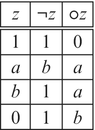
Example 2.17 (BALFIs over $\wp (\{w_1,w_2\})$ ).

Let $\mathcal {A}_4=\wp (\{w_1,w_2\}) = \{0, a,b,1\}$ be the powerset of $W_2=\{w_1,w_2\}$ such that $0=\emptyset $ , $a=\{w_1\}$ , $b=\{w_2\}$ and $1=\{w_1,w_2\}$ . Then, the BALFIs defined by expanding the Boolean algebra $\mathcal {A}_4$ are shown in Figure 1.

Fig. 1

Set of BALFIs over $\mathcal {A}_4$ (the symbol $|$ separates the possible options for the values of $\neg z$ and ${\circ } z$ for every value of z, while x stands for any element of $\mathcal {A}_4$ ).

On each row of Figure 1, each choice in the ith position of the sequence of options in the column for $\neg z$ forces a choice in the ith position of the sequence of options in the column for ${\circ } z$ . For instance, if in the current BALFI we choose $\neg 1=b$ then there are two possibilities for the value of ${\circ } 1$ in that BALFI: either ${\circ } 1=0$ or ${\circ } 1=a$ . On the other hand, by choosing that $\neg a=1$ it forces that either ${\circ } a=0$ or ${\circ } a=b$ . Otherwise, if $\neg a=b$ then ${\circ } a$ can be arbitrarily chosen.

Remark 2.18. Observe that the rules $(\textbf {R}_\neg )\ \text{and}\ (\textbf {R}_\circ )$ do not ensure that $ \vdash _{\mathbf {RmbC}} (\alpha \leftrightarrow \beta ) \to (\neg \alpha \leftrightarrow \neg \beta )$ and $ \vdash _{\mathbf {RmbC}} (\alpha \leftrightarrow \beta ) \to ({\circ }\alpha \leftrightarrow {\circ }\beta )$ in general. Consider, for instance $\alpha =p$ and $\beta =q$ where p and q are two different propositional variables, and take the BALFI $\mathcal {B}$ (in Figure 2) defined over the Boolean algebra $\wp (\{w_1,w_2\})$ , according to Example 2.17.

Fig. 2

Counter-model BALFI (over $\mathcal {A}_4$ ) for $\vdash _{\mathbf {RmbC}} (\alpha \leftrightarrow \beta ) \to (\#\alpha \leftrightarrow \#\beta )$ ; $\#\in \{\neg , \circ \}$ .

Now, consider a valuation v over $\mathcal {B}$ such that $v(p)=a$ and $v(q)=1$ . Hence $v(\neg p)=b$ , $v(\neg q)=1$ , $v({\circ } p)=a$ and $v({\circ } q) = 0$ . From this $v(p \leftrightarrow q)=a$ and $v(\neg p \leftrightarrow \neg q)= v({\circ } p \leftrightarrow {\circ } q)= b$ . Therefore $v((p \leftrightarrow q) \to (\neg p \leftrightarrow \neg q))=v((p \leftrightarrow q) \to ({\circ } p \leftrightarrow {\circ } q)) =b$ . That is, none of the last two formulas is valid in RmbC. Of course both formulas hold if $\vdash _{\mathbf {RmbC}} (\alpha \leftrightarrow \beta )$ , by $(\textbf {R}_\neg )$ and $(\textbf {R}_\circ )$ .

Evidently, RmbC is paraconsistent: in the BALFI $\mathcal {B}$ we just defined above, the given valuation v shows that $q,\neg q \nvdash _{\mathbf { RmbC}} p$ . Now, recalling Definition 2.1, RmbC is clearly an LFI. Consider the following BALFI $\mathcal {B}^{\prime }$ (in Figure 3) defined over $\wp (\{w_1,w_2\})$ , using again Example 2.17.

Fig. 3

BALFI (over $\mathcal {A}_4$ ) validating the principle of gentle explosion in a non-trivial way.

Take a valuation $v^{\prime }$ over $\mathcal {B}^{\prime }$ such that $v^{\prime }(p)=1$ and $v^{\prime }(q)=a$ . This shows that $p,{\circ } p \nvdash _{\mathbf {RmbC}} q$ . Now, a valuation $v^{\prime \prime }$ over $\mathcal {B}^{\prime }$ such that $v^{\prime \prime }(p)=0$ and $v^{\prime \prime }(q)=b$ shows that $\neg p, {\circ } p \nvdash _{\mathbf {RmbC}} q$ . On the other hand, from axiom (bc1), the axioms of CPL $^+$ , and by Definition 2.5(3), it is the case that $\alpha , \neg \alpha , {\circ }\alpha \vdash _{\mathbf {RmbC}} \beta $ for any formulas $\alpha $ and $\beta $ .

3 Adding replacement to extensions of mbC: A solution to an open problem

In [Reference Carnielli, Marcos, Carnielli, Coniglio and D’Ottaviano24], the first study on LFIs, the replacement property was analyzed under the name (IpE), presented in the following (equivalent) way:

(IpE) if $\alpha _i \dashv \vdash \beta _i$ (for $1 \leq i \leq n$ ) then $\varphi (\alpha _1,\ldots ,\alpha _n) \dashv \vdash \varphi (\beta _1,\ldots ,\beta _n)$

for any formulas $\alpha _i, \beta _i, \varphi $ . In that paper an important question was posed: to define extensions of bC and Ci (two axiomatic extensions of mbC to be analyzed below) which satisfy (IpE) while still being paraconsistent.Footnote ⁷ In this section, we will present a general (in the sense of minimal) solution to that open problem, obtained by extending axiomatically RmbC. In what follows, some LFIs which are axiomatic extensions of mbC (bC and Ci, among others) will be enriched with replacement, in a similar way as we did for RmbC.

Definition 3.19 (Some extensions of mbC).

Consider the following axioms presented in [Reference Carnielli and Coniglio15, Reference Carnielli, Marcos, Carnielli, Coniglio and D’Ottaviano24]:

(ciw) $$\begin{align} {\circ}\alpha \lor (\alpha \land \lnot \alpha) \end{align}$$

(ci) $$\begin{align} \lnot{\circ}\alpha \rightarrow (\alpha \land \lnot \alpha) \end{align}$$

(cl) $$\begin{align} \lnot(\alpha \land \lnot \alpha) \rightarrow {\circ}\alpha \end{align}$$

(cf) $$\begin{align} \lnot\lnot\alpha \rightarrow \alpha \end{align}$$

(ce) $$\begin{align} \alpha \rightarrow \lnot\lnot\alpha \end{align}$$

(ca _⩓) $$\begin{align} ({\circ}\alpha \land {\circ}\beta) \rightarrow {\circ}(\alpha\land \beta) \end{align}$$

(ca _∨) $$\begin{align} ({\circ}\alpha \land {\circ}\beta) \rightarrow {\circ}(\alpha\lor \beta) \end{align}$$

(ca ^→) $$\begin{align} ({\circ}\alpha \land {\circ}\beta) \rightarrow {\circ}(\alpha\rightarrow \beta) \end{align}$$

As mentioned in Remark 2.11 the Boolean complement in Boolean algebras defined over the signature $\Sigma _{BA}$ is given by ${\sim } a = a \to 0$ .

Let $Ax$ be a set formed by one or more of the axiom schemas introduced in Definition 3.19, and let $\mathbf {mbC}(Ax)$ be the logic defined by the Hilbert calculus obtained from mbC by adding the set $Ax$ of axiom schemas. Let $\mathbb {BI}(Ax)$ be the class of BALFIs which are models of every axiom in $Ax$ . Clearly, $\mathbb {BI}(Ax)$ is a variety of algebras, since it is characterized by a set of equations. Finally, let $\mathbf {RmbC}(Ax)$ be the logic obtained from RmbC by adding the set $Ax$ of axiom schemas. It is simple to adapt the proofs of Theorems 2.14 and 2.15 (in particular, by defining for each logic the corresponding canonical model, as in Definition 2.16) in order to obtain the following:

From this important result, some properties of the calculi $\mathbf {RmbC}(Ax)$ can be easily proven by algebraic methods, that is, by means of BALFIs. For instance:

It is also interesting to observe that ${\circ }$ satisfies a sort of necessitation rule (by analogy to modal logics) in certain extensions of RmbC:

Proposition 3.26. Consider the necessitation rule for $\circ $ :

$$ \begin{align*}\frac{\alpha}{{\circ}\alpha} \hspace{8mm} (Nec_{\circ})\end{align*} $$

Then, $(Nec_{\circ })$ is an admissible rule in $\mathbf {RmbC}(\{\mathbf {cl},\mathbf {ce}\})$ .Footnote ⁹

We can now provide a solution to the first open problem posed in [Reference Carnielli, Marcos, Carnielli, Coniglio and D’Ottaviano24]:

Example 3.27 (A paraconsistent extension of bC with replacement).

Consider the logic bC introduced in [Reference Carnielli, Marcos, Carnielli, Coniglio and D’Ottaviano24]. By using the notation proposed above, bC corresponds to mbC(cf).Footnote ¹⁰ Then RbC (that is, RmbC(cf)) is an extension of bC which satisfies replacement (by Theorem 2.8) while being still paraconsistent. Moreover, RbC is an LFI. These facts can be easily proven by using the BALFI $\mathcal {B}^{\prime }$ defined over $\wp (\{w_1,w_2\})$ considered in Remark 2.18 (see Figure 4).

Fig. 4

A four-element paraconsistent BALFI for RbC.

In fact, it is immediate to see that $\mathcal {B}^{\prime }$ is a model of $(\mathbf {cf})$ . It is worth noting that $\mathcal {B}^{\prime }$ is not a model of $(\mathbf {ciw})$ : $0={\circ } a \neq {\sim }(a\wedge \neg a)={\sim } a =b$ . Therefore, $\mathcal {B}^{\prime }$ is neither a model of $(\mathbf {ci})$ nor of $(\mathbf {cl})$ , given that any of these axioms implies $(\mathbf {ciw})$ .

We can now offer a solution to the second open problem posed in [Reference Carnielli, Marcos, Carnielli, Coniglio and D’Ottaviano24]:

Example 3.28 (A paraconsistent extension of Ci with replacement).

Now, consider the logic Ci introduced in [Reference Carnielli, Marcos, Carnielli, Coniglio and D’Ottaviano24], which corresponds to mbC({cf, ci}), and let RCi=RmbC({cf, ci}). By Proposition 3.24, RCi also derives the schema $(\mathbf {cl})$ . It can be proven that RCi is an extension of Ci which satisfies replacement (by Theorem 2.8) while it is still paraconsistent. In order to prove this, consider the BALFI $\mathcal {B}^{\prime \prime }$ defined over the Boolean algebra $\mathcal {A}_{16}=\wp (W_4)$ , the powerset of $W_4=\{w_1,w_2,w_3,w_4\}$ displayed in Figure 5. In that figure, X is different from $\{w_1,w_2\}$ and $\{w_3,w_4\}$ (note that $0=\emptyset $ and $1=W_4$ ). It is immediate to see that $\mathcal {B}^{\prime \prime }$ is a BALFI for RCi. Hence, using this model it follows easily that RCi is a paraconsistent extension of Ci which satisfies (IpE) and $(\mathbf {cl})$ .

Fig. 5

A 16-element paraconsistent BALFI for RCi.

Another paraconsistent model for RCi defined over $\mathcal {A}_{16}$ is displayed in Figure 6. Here, the cardinal of X is different from $2$ .Footnote ¹¹

Fig. 6

Another 16-element paraconsistent BALFI for RCi.

Example 3.29. We can offer now a model of RmbC(cl) that does not satisfy axiom $(\mathbf {cf})$ . For this purpose consider the BALFI $\mathcal {B}^{\prime \prime \prime }$ defined over the Boolean algebra $\mathcal {A}_4=\wp (\{w_1,w_2\}) = \{0, a,b,1\}$ according to Example 2.17, and displayed in Figure 7. Observe that $\mathcal {B}^{\prime \prime \prime } \Vdash \mathbf {cl}$ . However, $\mathcal {B}^{\prime \prime \prime }$ is not a model of $(\mathbf {cf})$ : $\neg \neg 0 = a \not \leq 0$ .

Fig. 7

A paraconsistent BALFI model of RmbC(cl) that does not satisfy axiom $(\mathbf {cf})$ .

4 Limits for replacement while preserving paraconsistency

In [Reference Carnielli, Marcos, Carnielli, Coniglio and D’Ottaviano24, Theorem 3.51] some sufficient conditions were given to show that certain extensions of bC and Ci cannot satisfy replacement while being still paraconsistent. This result shows that there are limits, much before reaching classical logic CPL, for extending RmbC while preserving paraconsistency. This result will now be applied in order to obtain two important examples of LFIs that cannot be extended with replacement at risk of losing their character of paraconsistency.

The first example, to begin with, is in fact a family of 8192 examples:

The second example deals with the well-known da Costa logic $C_1$ .

The failure of finding a paraconsistent extension of $C_1$ enjoying (IpE) was first observed in [Reference Urbas62, Chap. Reference Avron, Zamansky, Beklemishev, Demri and Máté5, Theorem 9], by proving that the extension of $C_n$ by replacement collapses to classical logic (see also [Reference Urbas63, Theorem 9] and [Reference Sylvan60, Sec. 4]).

5 Neighborhood semantics for RmbC

In this section we will introduce a particular case of BALFIs based on powerset Boolean algebras. These structures are in fact equivalent to neighborhood frames for non-normal modal logics, as we shall see in Section 6. Moreover, we shall prove in that section that, with this semantics, RmbC can be defined within the bimodal version of the minimal modal logic E (also termed classical modal logic in [Reference Chellas25, Definition 8.1]).

Clearly $\lbrack \!\lbrack \varphi \rbrack \!\rbrack \cup \lbrack \!\lbrack \neg \varphi \rbrack \!\rbrack = W$ , but $\lbrack \!\lbrack \varphi \rbrack \!\rbrack \cap \lbrack \!\lbrack \neg \varphi \rbrack \!\rbrack $ is not necessarily empty. In addition, $\lbrack \!\lbrack \varphi \rbrack \!\rbrack \cap \lbrack \!\lbrack \neg \varphi \rbrack \!\rbrack \cap \lbrack \!\lbrack {\circ }\varphi \rbrack \!\rbrack = \emptyset $ . Intuitively, the functions $S_\neg $ and $S_{\circ }$ act as ‘regulators’ for the values given to the non-standard connectives $\neg $ and ${\circ }$ . Indeed, $S_\neg (\lbrack \!\lbrack \varphi \rbrack \!\rbrack )$ is the value to be ‘added’ to the value of the classical negation of $\varphi $ (that is, the Boolean complement of $\lbrack \!\lbrack \varphi \rbrack \!\rbrack $ ) in order to allow paraconsistency. In fact, in RmbCciw and its extensions the value of ${\circ }\varphi $ is the Boolean complement of the value of the contradiction $\varphi \land \neg \varphi $ . However, in RmbC the value of ${\circ }\varphi $ could be less than this, and thus it becomes ‘decreased’ by intersection with $S_{\circ }(\lbrack \!\lbrack \varphi \rbrack \!\rbrack )$ .

Clearly, $\Gamma \models _{\mathbb {NM}} \varphi $ if either $\lbrack \!\lbrack \varphi \rbrack \!\rbrack _{\mathcal {M}} = W$ for every neighborhood model $\mathcal {M}$ for RmbC, or there exists a finite, non-empty subset $\{\gamma _1,\ldots ,\gamma _n\}$ of $\Gamma $ such that, for every neighborhood model $\mathcal {M}$ for RmbC, $\bigcap _{i=1}^n\lbrack \!\lbrack \gamma _i \rbrack \!\rbrack _{\mathcal {M}} \subseteq \lbrack \!\lbrack \varphi \rbrack \!\rbrack _{\mathcal {M}}$ .

Proposition 5.35 suggests the following:

In order to prove completeness of RmbC w.r.t. neighborhood models, Stone’s representation theorem for Boolean algebras will be used. This important theorem, first proved in [Reference Stone59], states that every Boolean algebra is isomorphic to a Boolean subalgebra of $\wp (W)$ , for a suitable W. This means that, given a Boolean algebra $\mathcal {A}$ , there exists a set W and an injective homomorphism $i:\mathcal {A} \to \wp (W)$ of Boolean algebras. Note that $i(a)=W$ if and only if $a= 1$ .

Proof. Let $\mathcal {A}_{can}$ be the Boolean algebra with carrier $A_{can}=For(\Sigma )/_{\equiv }$ , and let $\mathcal {B}_{can}$ be the corresponding expansion to $\Sigma _e$ , as defined in the proof of Theorem 2.15. Let $i:\mathcal {A}_{can} \to \wp (W)$ be an injective homomorphism of Boolean algebras, according to Stone’s theorem as discussed above. Consider the neighborhood frame $\mathcal {F}_{can}=\langle W, S_\neg ,S_{\circ }\rangle $ for RmbC such that the functions $S_\neg $ and $S_{\circ }$ satisfy the following: $S_\neg (i([\alpha ])) = i([\neg \alpha ])$ , and $S_{\circ }(i([\alpha ])) = {i}([{\circ }\alpha ])$ , for every formula $\alpha $ (where $[\alpha ]$ denotes the equivalence class of $\alpha $ w.r.t. ${\equiv }$ ). Observe that these functions are well-defined, since every connective in RmbC is congruential and i is injective. The values of these functions outside the image of i can be arbitrary. Now, let $\mathcal {M}_{can}=\langle \mathcal {F}_{can},d_{can}\rangle $ be the neighborhood model for RmbC such that $d_{can}(p)~\stackrel {\text {{ def }}}{=}~{i}([p])$ , for every propositional variable p.

Fact: $\lbrack \!\lbrack \alpha \rbrack \!\rbrack _{\mathcal {M}_{can}}=i([\alpha ])$ , for every formula $\alpha $ .

The proof of the Fact will be done by induction on the complexity of the formula $\alpha $ (recalling Definition 5.33 for $\lbrack \!\lbrack \cdot \rbrack \!\rbrack _{\mathcal {M}}$ ). The complexity of ${\circ }\alpha $ is taken to be strictly greater than the complexity of $\neg \alpha $ . The case for $\alpha $ atomic or $\alpha =\beta \# \gamma $ for $\# \in \{\wedge ,\vee ,\to \}$ is clear, by the very definitions and by induction hypothesis. Now, suppose that $\alpha =\neg \beta $ . By induction hypothesis, $\lbrack \!\lbrack \beta \rbrack \!\rbrack =i([\beta ])$ . Observe that ${\sim }[\beta ] \leq [\neg \beta ]$ in $\mathcal {A}_{can}$ (where ${\sim }$ denotes the Boolean complement in $\mathcal {A}_{can}$ ); hence, $W\setminus i([\beta ]) = i({\sim }[\beta ]) \subseteq i([\neg \beta ])$ . Thus,

$$\begin{align*}\lbrack \!\lbrack \neg \beta \rbrack \!\rbrack &= (W \setminus \lbrack \!\lbrack \beta \rbrack \!\rbrack ) \cup S_\neg (\lbrack \!\lbrack \beta \rbrack \!\rbrack )=(W \setminus i([\beta ])) \cup S_\neg (i([\beta ]))\\ &=(W \setminus i([\beta ])) \cup i([\neg \beta ]) = i([\neg \beta ]) \end{align*}$$

Finally, let $\alpha ={\circ }\beta $ . Since $[{\circ }\beta ] \leq {\sim }([\beta ] \wedge [\neg \beta ])$ in $\mathcal {A}_{can}$ then $i([{\circ }\beta ]) \subseteq W \setminus (i([\beta ]) \cap i([\neg \beta ]))$ . Hence, by induction hypothesis,

$$\begin{align*}\lbrack \!\lbrack {\circ }\beta \rbrack \!\rbrack &= (W \setminus (i([\beta ]) \cap i([\neg \beta ]))) \cap S_{\circ }(i([\beta ])\\ &=(W \setminus (i([\beta ]) \cap i([\neg \beta ]))) \cap i([{\circ }\beta ]) = i([{\circ }\beta ]). \end{align*}$$

This concludes the proof of the Fact.

Because of the Fact, $\mathcal {M}_{can} \Vdash \alpha $ iff $i([\alpha ])=W$ iff $[\alpha ]=1$ iff $\vdash _{\mathbf {RmbC}} \alpha $ . Now, suppose that $\Gamma \models _{\mathbb {NM}} \varphi $ . If $\models _{\mathbb {NM}} \varphi $ then, in particular, $\mathcal {M}_{can} \Vdash \varphi $ and so $\vdash _{\mathbf {RmbC}} \varphi $ . From this, $\Gamma \vdash _{\mathbf {RmbC}} \varphi $ . On the other hand, suppose that there exists a finite, non-empty subset $\{\gamma _1,\ldots ,\gamma _n\}$ of $\Gamma $ such that $\models _{\mathbb {NM}} (\gamma _1 \wedge \cdots \wedge \gamma _n) \to \varphi $ . By reasoning as above, it follows that $\vdash _{\mathbf {RmbC}} (\gamma _1 \wedge \cdots \wedge \gamma _n) \to \varphi $ and so $\Gamma \vdash _{\mathbf {RmbC}} \varphi $ as well.□

6 RmbC is definable within the minimal bimodal modal logic

This section shows that RmbC is definable within the bimodal version of the minimal modal logic E, also called classical modal logic in [Reference Chellas25, Definition 8.1]. In terms of combination of modal logics, this bimodal logic is equivalent to the fusion (or, equivalently, the constrained fibring by sharing the classical connectives) of E with itself.Footnote ¹² This means that the minimal non-normal modal logic with two independent modalities $\square _1$ and $\square _2$ , which will be denoted by $\mathbf {E}{\oplus }\mathbf {E}$ , contains RmbC, the minimal self-extensional LFI. As we shall see, in the case of RmbC both modalities are required for defining the two non-classical connectives $\neg $ and $\circ $ . For RmbCciw and its extensions only one modality is needed, since $\circ $ can be taken as a derived operator (recall Example 3.25). Hence RmbCciw is definable in E.

The minimal (or classical) modal logic E was introduced by Montague [Reference Montague51] and Scott [Reference Scott and Lambert56] with semantics given by neighborhood models, which generalize the usual Kripke models for modal logic. Neighborhood semantics has become one of the main mechanisms for providing semantics for non-normal modal logics as well as for some normal modal logics that are not complete w.r.t. Kripke models (see, e.g., [Reference Gabbay41]). Among the first important applications of neighborhood semantics we count the well-known book on counterfactual conditionals by [Reference Lewis46]. Ever since, it has found many successful applications in areas of conditional, deontic, and epistemic logic (see, e.g., [Reference Pacuit55]). For convenience, the definition of modal logic E will be briefly surveyed below.

Let $\Sigma _m=\{\land , \lor , \to , {\sim }, \square , \lozenge \}$ and $\Sigma _{bm}=\{\land , \lor , \to , {\sim }, \square _1,\lozenge _1,\square _2,\lozenge _2\}$ be the signatures introduced in Definition 2.2. The class of models $\mathcal {C_M}$ induces a modal consequence relation defined as follows:

A formula $\varphi $ is true in $\mathcal {N}$ if $\lbrack \!\lbrack \varphi \rbrack \!\rbrack ^{\mathcal {N}} = W$ , and it is valid w.r.t. $\mathcal {C_M}$ , denoted by $\models ^{\mathcal {C_M}} \varphi $ , if it is true in every minimal model. The degree-preserving consequence w.r.t. $\mathcal {C_M}$ can be defined analogously to the one for neighborhood semantics for RmbC given in Definition 5.34. Namely, $\Gamma \models ^{\mathcal {C_M}} \varphi $ if either $\models ^{\mathcal {C_M}} \varphi $ , or there exists a finite, non-empty subset $\{\gamma _1,\ldots ,\gamma _n\}$ of $\Gamma $ such that $\models ^{\mathcal {C_M}}(\gamma _1 \wedge \cdots \wedge \gamma _n) \to \varphi $ . The latter is equivalent to $\bigcap _{i=1}^n \lbrack \!\lbrack \gamma _i \rbrack \!\rbrack ^{\mathcal {N}} \subseteq \lbrack \!\lbrack \varphi \rbrack \!\rbrack ^{\mathcal {N}}$ .

Definition 6.41 ([Reference Chellas25, Definition 8.1]).

The minimal modal logic (or classical modal logic) E is defined by means of a Hilbert calculus over the signature $\Sigma _m$ obtained by adding to the Hilbert calculus for CPL $^+$ (recall Definition 2.3) the following axiom schemas and rules:

(PEM) $$\begin{align} \alpha \lor {\sim} \alpha \end{align}$$

(exp) $$\begin{align} \alpha \rightarrow \big({\sim} \alpha \rightarrow \beta\big) \end{align}$$

(AxMod) $$\begin{align} \lozenge\alpha \leftrightarrow {\sim}\square{\sim}\alpha \end{align}$$

(R□) $$\begin{align} \frac{\alpha \leftrightarrow \beta}{\square\alpha \leftrightarrow \square\beta} \end{align}$$

The notion of derivation in E is defined as for RmbC, recall Definition 2.6. Note that (PEM) and (exp), together with CPL $^+$ , guarantee that E is an expansion of propositional classical logic by adding the modalities $\square $ and $\lozenge $ which are interdefinable as usual, and such that both are congruential. That is, E satisfies replacement.

Definition 6.43 (Minimal bimodal logic).

The minimal bimodal logic $\mathbf {E} {\oplus } \mathbf {E}$ is defined by means of a Hilbert calculus over signature $\Sigma _{bm}$ obtained by adding to the Hilbert calculus for CPL $^+$ the following axiom schemas and rules, for $i=1,2$ :

(PEM) $$\begin{align} \alpha \lor {\sim} \alpha \end{align}$$

(exp) $$\begin{align} \alpha \rightarrow \big({\sim} \alpha \rightarrow \beta\big) \end{align}$$

(AxModi) $$\begin{align} \lozenge_i\alpha \leftrightarrow {\sim}\square_i{\sim}\alpha \end{align}$$

(R□i) $$\begin{align} \frac{\alpha \leftrightarrow \beta}{\square_i\alpha \leftrightarrow \square_i\beta} \end{align}$$

Observe that $\mathbf {E} {\oplus } \mathbf {E}$ is obtained from E by ‘duplicating’ the modalities. There is no relationship between $\square _1$ and $\square _2$ and so $\lozenge _1$ and $\lozenge _2$ are also independent.

The semantics of $\mathbf {E} {\oplus } \mathbf {E}$ is given by the class $\mathcal {C^{\prime }_M}$ of structures of the form $\mathcal {N} = \langle W, N_1,N_2,d \rangle $ such that W is a non-empty set and $N_i:W \to \wp (\wp (W))$ (for $i=1,2$ ) and $d:\mathcal {V} \to \wp (W)$ are functions. The denotation $\lbrack \!\lbrack \varphi \rbrack \!\rbrack ^{\mathcal {N}}$ of a formula $\varphi \in For(\Sigma _{bm})$ in $\mathcal {N}$ is defined by an obvious adaptation of Definition 6.40 to $For(\Sigma _{bm})$ . By defining the consequence relations $\vdash _{\mathbf {E} {\oplus } \mathbf {E}}$ and $\models ^{\mathcal {C^{\prime }_M}}$ in analogy to the ones for E, it is straightforward to adapt the proof of soundness and completeness of E to the bimodal case.

From the point of view of combining logics, $\mathbf {E} {\oplus } \mathbf {E}$ is the fusion (or, equivalently, the constrained fibring by sharing the classical connectives) of E with itself (see [Reference Carnielli, Coniglio and Zalta17, Reference Carnielli, Coniglio, Gabbay, Gouveia and Sernadas19]).

Finally, it will be shown that RmbC can be defined inside $\mathbf {E}{\oplus } \mathbf {E}$ by means of the following abbreviations, which are motivated by Definition 5.33 (having in mind that $\square _1$ and $\square _2$ will be interpreted by the mappings $S_\neg $ and $S_\circ $ , respectively):

$$ \begin{align*}\neg \varphi ~\stackrel{\text{{ def }}}{=}~ \varphi \to \square_1 \varphi \ \text{ and } \ {\circ} \varphi ~\stackrel{\text{{ def }}}{=}~ {\sim}(\varphi \land \square_1 \varphi) \land \square_2 \varphi.\end{align*} $$

In order to see this, observe that any function $N:W \to \wp (\wp (W))$ induces a unique function $S:\wp (W) \to \wp (W)$ given by $S(X) = \{w \in W \ : \ X \in N(w)\}$ . Conversely, any function $S:\wp (W) \to \wp (W)$ induces a function $N:W \to \wp (\wp (W))$ given by $N(w) = \{X \subseteq W \ : \ w \in S(X)\}$ . Both assignments $N \mapsto S$ and $S \mapsto N$ are inverses of each other. From this, a structure (or minimal model) $\mathcal {N} = \langle W, N_1,N_2, d \rangle $ for $\mathbf {E} {\oplus } \mathbf {E}$ can be transformed into a neighborhood model $\mathcal {M}=\langle W, S_\neg ,S_{\circ },d\rangle $ for RmbC such that $S_\neg $ and $S_{\circ }$ are obtained, respectively, from the functions $N_1$ and $N_2$ as indicated above. Observe that

$$ \begin{align*}w \in \lbrack\!\lbrack \square_1\varphi \rbrack\!\rbrack^{\mathcal{N}} \ \text{ iff } \ \models^{\mathcal{N}}_w \square_1 \varphi \ \text{ iff } \ \lbrack\!\lbrack \varphi \rbrack\!\rbrack^{\mathcal{N}} \in N_1(w) \ \text{ iff } \ w \in S_\neg(\lbrack\!\lbrack \varphi \rbrack\!\rbrack^{\mathcal{N}}).\end{align*} $$

That is, $S_\neg (\lbrack \!\lbrack \varphi \rbrack \!\rbrack ^{\mathcal {N}}) = \lbrack \!\lbrack \square _1\varphi \rbrack \!\rbrack ^{\mathcal {N}}$ . Analogously, $S_{\circ }(\lbrack \!\lbrack \varphi \rbrack \!\rbrack ^{\mathcal {N}}) = \lbrack \!\lbrack \square _2\varphi \rbrack \!\rbrack ^{\mathcal {N}}$ . From this, it is easy to prove by induction on the complexity of the formula $\varphi \in For(\Sigma )$ that $\lbrack \!\lbrack \varphi \rbrack \!\rbrack _{\mathcal {M}}=\lbrack \!\lbrack \varphi ^t \rbrack \!\rbrack ^{\mathcal {N}}$ , where $\varphi ^t$ is the formula over the signature $\Sigma _{bm}$ obtained from $\varphi $ by replacing any occurrence of the connectives $\neg $ and ${\circ }$ by the corresponding abbreviations, as indicated above. Conversely, any neighborhood model $\mathcal {M}=\langle W, S_\neg ,S_{\circ },d\rangle $ for RmbC gives origin to a unique minimal model $\mathcal {N} = \langle W, N_1,N_2, d \rangle $ for $\mathbf {E} {\oplus } \mathbf {E}$ such that $\lbrack \!\lbrack \varphi \rbrack \!\rbrack _{\mathcal {M}}=\lbrack \!\lbrack \varphi ^t \rbrack \!\rbrack ^{\mathcal {N}}$ for every formula $\varphi \in For(\Sigma )$ . That is, the class of minimal models for $\mathbf {E} {\oplus } \mathbf {E}$ coincides (up to presentation) with the class of neighborhood models for RmbC, and both classes validate the same formulas over the signature $\Sigma $ of RmbC. From this, Corollary 5.36, and Theorems 5.38 and 6.44 we show that RmbC is definable within $\mathbf {E} {\oplus } \mathbf {E}$ :

The main result obtained in this section, namely Theorem 6.45, establishes an interesting relation between non-normal modal logics and paraconsistent logics.

Connections between modalities and paraconsistency, or proposals emphasizing a connection between negations, denial, and impossibility, are well-known in the literature. Segerberg [Reference Segerberg57, p. 128] suggests the possibility of studying the (unexplored at that time) modal notion of ‘ $\varphi $ is non-necessary’, namely ${\sim }\square \varphi $ . Along the same lines, Došen [Reference Došen34] investigates modal operators corresponding to impossibility and non-necessity in systems analogous to the modal system K based on intuitionistic (instead of classical) logic. A system where impossibility is equivalent to intuitionistic negation is also investigated (proving soundness and completeness). Došen [Reference Došen35] investigates negation as a modal impossibility operator added to a negationless logic. In turn, Vakarelov [Reference Vakarelov, Priest, Routley and Norman64]Footnote ¹³ builds upon a distributive (lattice) logic to introduce a class of negations (generalizing intuitionistic negation) termed regular negations by drawing upon the notion of theory consistency/compatibility. Some convenient semantical simplifications giving rise to the special subclasses of normal and standard negations are also discussed. In an analogous manner, by drawing upon the dual notion of theory completeness, Vakarelov introduces the dual class of co-regular (as well as co-normal and co-standard) negations. Vakarelov also discusses paraconsistent and paracomplete negations and relates them to particular subclasses of regular and co-regular logics. Along similar lines, Dunn & Zhou [Reference Dunn and Zhou38] (drawing upon [Reference Dunn36]) study two families of negative modal operators interpreted as impossibility and (dually) as non-necessity, each represented in an ordered structure termed “(dual) kite of negations.”

More recently, Béziau [Reference Béziau9, Reference Béziau10] proposes to examine a paraconsistent negation defined in the modal system S5 as $\neg \varphi ~\stackrel {\text {{ def }}}{=}~ \lozenge {\sim } \varphi $ (which is equivalent to ${\sim }\square \varphi $ ). Historically situated between the early works by Došen and Vakarelov mentioned above and Béziau’s proposal, a similar way of defining a paraconsistent negation inside a modal logic has been regarded in [Reference de Araújo, Alves and Guerzoni33], where the authors propose a Kripke-style semantics for Sette’s three-valued paraconsistent logic P1 based on Kripke frames for the modal logic T. This result was improved in [Reference Carnielli, Lima-Marques, Carnielli and D’Ottaviano23], by showing that P1 can be interpreted in T by means of Kripke frames having at most two worlds.

Several authors have explored the possibility of defining such paraconsistent negation in other modal logics such as B [Reference Avron, Zamansky, Beklemishev, Demri and Máté5], S4 [Reference Coniglio, Prieto-Sanabria, Gouveia, Carlos and Donisio27] and even weaker modal systems [Reference Bueno-Soler, Carnielli, Markin and Zaitsev14]. In such context, Marcos [Reference Marcos50] proposes, besides the paraconsistent negation defined as above, the definition of a consistency connective within a modal system by means of the formula ${\circ }\varphi ~\stackrel {\text {{ def }}}{=}~ \varphi \to \square \varphi $ . In that paper it is shown that any normal modal logic in which the schema $\varphi \to \square \varphi $ is not valid gives origin to an LFI in this way. Moreover, it is shown that it is also possible to start from a “modal LFI,” over the signature $\Sigma $ of LFIs, in which the paraconsistent negation and the consistency connective feature a Kripke-style semantics, defining the modal necessity operator by means of the formula $\square \varphi ~\stackrel {\text {{ def }}}{=}~ {\sim }\lnot \varphi $ (where ${\sim }$ is the strong negation defined in terms of $\lnot $ and ${\circ }$ as in mbC, recall Remark 3.20(2)). This shows that ‘reasonable’ normal modal logics and LFIs with Kripke-style semantics are two faces of the same coin.

Our Theorem 6.45 partially extends this relationship to the realm of non-normal modal logics. The result we have obtained is partial, in the sense that the minimum bimodal non-normal modal logics gives origin to RmbC, but the converse does not seem to be true. Namely, starting from RmbC it is not obvious that the modalities $\square _1$ and $\square _2$ could be defined by means of formulas in the signature $\Sigma $ . This topic deserves further investigation.

7 Neighborhood models for axiomatic extensions of RmbC

In this section $Ax$ will denote a set formed by one or more of the axiom schemas introduced in Definition 3.19 with the exception of (ca $_\#$ ) for $\# \in \{\land , \vee , \to \}$ (given the limitations to paraconsistency imposed to logic RCila (recall Example 4.31). Let $\mathbb {NM}(Ax)$ the class of neighborhood frames in which every schema in $Ax$ is valid. Define the consequence relation $\models _{\mathbb {NM}(Ax)}$ in the obvious way. By adapting the previous results it is easy to prove the following:

The class of neighborhood frames that validates each of the axioms of $Ax$ can be easily characterized:

Recall the minimal bimodal logic $\mathbf {E} {\oplus } \mathbf {E}$ studied in Section 6. If $\varphi $ is a formula in $For(\Sigma _{bm})$ then $\mathbf {E} {\oplus } \mathbf {E}(\varphi )$ will denote the extension of $\mathbf {E} {\oplus } \mathbf {E}$ by adding $\varphi $ as an axiom schema. Let $\mathcal {C^{\prime }_M}(\varphi )$ be the class of structures (i.e., minimal models) $\mathcal {N}$ for $\mathbf {E} {\oplus } \mathbf {E}$ such that $\varphi $ is valid in $\mathcal {N}$ (as an axiom schema). Theorem 6.44 can be extended to prove that the logic $\mathbf {E} {\oplus } \mathbf {E}(\varphi )$ is sound and complete w.r.t. the semantics in $\mathcal {C^{\prime }_M}(\varphi )$ . From this, and taking into account the representability of RmbC within $\mathbf {E} {\oplus } \mathbf {E}$ (Theorem 6.45) and the equivalence between minimal models for $\mathbf {E} {\oplus } \mathbf {E}$ and neighborhood models for RmbC discussed right before Theorem 6.45, Proposition 7.47 can be recast as follows:

We have, in fact, that $\mathbf {RmbC}(\mathbf {ciw})$ and its extension $\mathbf {RmbC}(\mathbf {ci})$ are definable in E. Recall from Example 3.25 that for them $\circ $ can be defined as a derived operator.

8 Truth-preserving (or global) semantics

As mentioned in Section 2, the BALFI semantics for RmbC, as well as its neighborhood semantics presented in Section 5, is degree-preserving instead of truth-preserving (using the terminology from [Reference Bou, Esteva, Font, Gil, Godo and Verdú13]). This requires adapting, in a coherent way, the usual definition of derivation from premises in a Hilbert calculus (recall Definition 2.6). This is in fact the methodology adopted with most normal modal logics in which the semantics is local, thus recovering the deduction metatheorem. But it is also possible to consider global (or truth-preserving) semantics, as it is usually done with algebraic semantics. This leads us to propose the logic $\mathbf {RmbC}^*$ , which is defined by the same Hilbert calculus than the one for RmbC, but now derivations from premises in $\mathbf {RmbC}^*$ are defined as usual in Hilbert calculi.

Now, the degree-preserving BALFI semantics for RmbC given in Definition 2.12 is replaced by a truth-preserving consequence relation for $\mathbf {RmbC}^*$ . Notice, however that, by virtue of the self-extensionality, this semantical notion will not require finitariness by definition: indeed, after proving soundness and completeness, finitariness of the semantical consequence relation (that is, the semantical compactness theorem for $\mathbf { RmbC}^*$ ) will be obtained as a corollary.Footnote ¹⁴

The distinction between local and global reasoning has been studied by A. Sernadas and his collaborators (for a brief exposition see, for instance, [Reference Carnielli, Coniglio, Gabbay, Gouveia and Sernadas19, Sec. 2.3 in Chap. 2]). From the proof-theoretical perspective, the Hilbert calculi (called Hilbert calculi with careful reasoning in [Reference Carnielli, Coniglio, Gabbay, Gouveia and Sernadas19, Definition 2.3.1]) are of the form $H= \langle \Theta , R_g,R_l\rangle $ where $\Theta $ is a propositional signature and $R_g \cup R_l$ is a set of inference rules such that $R_l \subseteq R_g$ and no element of $R_g\setminus R_l$ is an axiom schema. Elements of $R_g$ and $R_l$ are called global and local inference rules, respectively. Given $\Gamma \cup \{\varphi \} \subseteq For(\Theta )$ , $\varphi $ is globally derivable from $\Gamma $ in H, written $\Gamma \vdash _H^g \varphi $ , if $\varphi $ is derivable from $\Gamma $ in the Hilbert calculus $\langle \Theta , R_g\rangle $ by using the standard definition (see Definition 8.50). On the other hand, in local derivations, besides using the local rules and the premises, global rules can be used provided that the premises are (global) theorems. In formal terms, $\varphi $ is locally derivable from $\Gamma $ in H, written $\Gamma \vdash _H^l \varphi $ , if there exists a finite sequence of formulas $\varphi _1\ldots \varphi _n$ such that $\varphi _n$ is $\varphi $ and, for every $1 \leq i \leq n$ , either $\varphi _i \in \Gamma $ , or $\vdash _H^g\varphi _i$ , or $\varphi _i$ is the consequence of some inference rule of $R_l$ whose premises appear in the sequence $\varphi _1\ldots \varphi _{i-1}$ (observe that this includes the case where $\varphi _i$ is an instance of an axiom in $R_l$ ). Obviously, local derivations are global derivations, but the converse does not necessarily hold: for instance, $\varphi \vdash _H^g \square \varphi $ always hold in a Hilbert calculus H for a normal modal logic (say, K), while $\varphi \vdash _H^l \square \varphi $ holds iff $\varphi $ is a theorem.Footnote ¹⁵ Clearly, local and global theorems coincide.

For instance, a Hilbert calculus for a (normal) modal logic typically contains, as local inference rules, (MP) and the axiom schemas, while the set of global rules is $(R_l)$ plus the necessitation rule. As we have seen in Section 6, for the minimal non-normal modal logic E we have a similar case, with the replacement rule for $\square $ being employed instead of the necessitation rule. In this case, the deduction metatheorem only holds for local derivations. Note that, by definition, derivations in $\mathbf {RmbC}^*$ lie in the scope of global derivations, while derivations in RmbC are local derivations. Hence, the extension of mbC with replacement can be recast as a Hilbert calculus with careful reasoning $\mathbf {RmbC}^ + = \langle \Sigma ,R_g,R_l\rangle $ such that $R_l$ contains the axiom schemas of mbC plus (MP), and $R_g$ contains, besides this, the rules $(\textbf {R}_\neg )$ and $(\textbf {R}_\circ )$ . Of course, the same can be done with the axiomatic extensions of mbC (and so of RmbC) considered in Section 3.

At the semantical level, local derivations correspond to degree-preserving semantics w.r.t. a given class $\mathbb {M}$ of algebras, while global derivations correspond to truth-preserving semantics w.r.t. the class $\mathbb {M}$ .

The presentation of LFIs with replacement as Hilbert calculi with careful reasoning (as the case of $\mathbf {RmbC}^ +$ ) can be useful in order to combine these logics with (standard) normal modal logics by algebraic fibring: in this case, completeness of the fibring of the corresponding Hilbert calculi w.r.t. a semantics given by classes of suitable expansions of Boolean algebras would be immediate, according to the results stated in [Reference Carnielli, Coniglio, Gabbay, Gouveia and Sernadas19, Chap. 2]. By considering, as done in [Reference Zanardo, Sernadas and Sernadas65], classes $\mathbb {M}$ of powerset algebras (i.e., with carrier of the form $\wp (W)$ for a non-empty set W) induced by Kripke models (which can be generalized to neighborhood models), then the fibring of, say, $\mathbf {RmbC}^ +$ with a given modal logic would simply be a minimal bimodal logic $\mathbf {E} {\oplus } \mathbf {E}$ with an additional modality $\square $ , from which we derive the following modalities: $\lozenge \varphi ~\stackrel {\text {{ def }}}{=}~ {\sim }\square {\sim }\varphi $ , $\neg \varphi ~\stackrel {\text {{ def }}}{=}~ \varphi \to \square _1\varphi $ , and ${\circ }\varphi ~\stackrel {\text {{ def }}}{=}~ {\sim }(\varphi \land \square _1\varphi ) \land \square _2\varphi $ . This opens interesting opportunities for future research.

9 Extension to first-order logics

The next step is extending RmbC, as well as its axiomatic extensions analyzed above, to first-order languages. We begin by extending the notion of a propositional signature to the first-order case.

The set $\mathcal {C}$ as well as any of $\mathcal {F}_n$ and $\mathcal {P}_n$ may be empty. However, $\bigcup _{n\geq 1}\mathcal {P}_n$ must be nonempty. In the sequel, we work with a fixed denumerable set $Var=\{v_1,v_2,\ldots \}$ of individual variables. The first-order language over $\Omega $ is defined as follows. The set of terms $Ter(\Omega )$ (resp. closed terms $CTer(\Omega )$ ) is freely generated by $Var\,\cup \,\mathcal {C}$ (resp. $\mathcal {C}$ ) employing the elements of $\;\bigcup _{n\geq 1}\mathcal {F}_n$ as connectives. The set of atomic formulas $AFor(\Omega )$ is composed of expressions of the form $P(\tau _1,\ldots ,\tau _n)$ where $P \in \mathcal {P}_n$ and $\tau _i \in Ter(\Omega )$ for $1\leq i \leq n$ . Finally, the set of formulas $For_1(\Omega )$ is freely generated by $AFor(\Omega )$ employing $\Sigma \cup \{\forall v\}_{v \in Var} \cup \{\exists v\}_{v \in Var}$ as connectives, where the latter two are $Var$ -indexed sets of quantifier symbols which we treat as having arity $1$ .

The set of closed formulas (or sentences) will be denoted by $Sen(\Omega )$ . The formula obtained from a given formula $\varphi $ by substituting every free occurrence of a variable x by a term t will be denoted by $\varphi [x/t]$ .

The consequence relation of RQmbC, suitably extending the one for RmbC (recall Definition 2.6) with the axioms and rules above, will be denoted by $\vdash _{\mathbf {RQmbC}}$ . Recall that a Hilbert calculus with careful reasoning for RmbC called $\mathbf {RmbC}^+$ was defined at the end of Section 8. This can be extended to the first-order case by considering the Hilbert calculus with careful reasoning $\mathbf {RQmbC}^+$ over a given first-order signature $\Omega $ , such that $R_l$ contains (MP) and the axiom schemas of mbC plus $\mathbf {(Ax\exists )}$ and $\mathbf {(Ax\forall )}$ . In turn, $R_g$ contains, besides the rules $R_l$ , the (global) rules $(\textbf {R}_\neg )$ , $(\textbf {R}_\circ )$ , $(\exists \textbf {-In}$ ) and $(\forall \textbf{-In})$ (over $\Omega $ ). The property of replacement for RQmbC follows directly from the propositional case (Theorem 2.8), observing that quantifiers (seen as unary operators) clearly preserve logical equivalence.

Given that, as in the case of RmbC, RQmbC uses local reasoning, it satisfies the deduction metatheorem without any restrictions. This is different from what happens with QmbC, a first-order version of mbC proposed in [Reference Carnielli, Coniglio, Podiacki and Rodrigues21], where this metatheorem holds with the same restrictions as in first-order classical logic.Footnote ¹⁶

10 BALFI semantics for RQmbC

In [Reference Coniglio, Figallo-Orellano and Golzio26] a semantics of first-order structures, based on swap structures over complete Boolean algebras, was obtained for QmbC. Since RQmbC is self-extensional, that semantics can be drastically simplified, and so the non-deterministic swap structures will be replaced by BALFIs, which are ordinary algebras. The semantics will be defined in an analogous fashion as we did for the propositional case, where valuations can be considered as homomorphisms between the algebra of formulas and BALFIs. In the sequel, only BALFIs over complete Boolean algebras will be considered. This requirement is justified since quantifiers will be interpreted by means of (infinite) infima and suprema in Boolean algebras; hence, their existence must be always guaranteed.

From now on, we will write $c^{\mathfrak {A}}$ , $f^{\mathfrak {A}}$ and $P^{\mathfrak {A}}$ instead of $I_{\mathfrak {A}}(c)$ , $I_{\mathfrak {A}}(f)$ and $I_{\mathfrak {A}}(P)$ to denote the interpretation of an individual constant symbol c, a function symbol f and a predicate symbol P, respectively.

Remark 10.64. (1) If t is a closed term we can write $\lbrack \!\lbrack t \rbrack \!\rbrack ^{\mathfrak {A}}$ instead of $\lbrack \!\lbrack t \rbrack \!\rbrack ^{\mathfrak {A}}_\mu $ , for any assignment $\mu $ , since it does not depend on $\mu $ . Analogously, we can write $\lbrack \!\lbrack \varphi \rbrack \!\rbrack ^{\mathfrak {A}}$ instead of $\lbrack \!\lbrack \varphi \rbrack \!\rbrack ^{\mathfrak {A}}_\mu $ for a closed formula $\varphi $ .

(2) The last two items can equivalently be written as:

$$ \begin{align*}(iv^*)\;\;\lbrack\!\lbrack \forall x\varphi \rbrack\!\rbrack^{\mathfrak{A}}_\mu = \bigwedge_{a \in U} \lbrack\!\lbrack \varphi \rbrack\!\rbrack^{\mathfrak{A}}_{\mu^x_a} \mathrm{\;\;\;\;\;\;and\;\;\;\;\;\;} (v^*)\;\;\lbrack\!\lbrack \exists x\varphi \rbrack\!\rbrack^{\mathfrak{A}}_\mu = \bigvee_{a \in U} \lbrack\!\lbrack \varphi \rbrack\!\rbrack^{\mathfrak{A}}_{\mu^x_a}\end{align*} $$

If x does not appear free in $\varphi $ we have that $\lbrack \!\lbrack \forall x\varphi \rbrack \!\rbrack ^{\mathfrak {A}}_\mu = \lbrack \!\lbrack \varphi \rbrack \!\rbrack ^{\mathfrak {A}}_\mu $ and $\lbrack \!\lbrack \exists x\varphi \rbrack \!\rbrack ^{\mathfrak {A}}_\mu = \lbrack \!\lbrack \varphi \rbrack \!\rbrack ^{\mathfrak {A}}_\mu $ .

In order to prove the soundness of RQmbC w.r.t. BALFI semantics, it is necessary to state an important result:

11 Completeness of RQmbC w.r.t. BALFI semantics

Along this section, in which the completeness of RQmbC w.r.t. BALFI semantics will be shown, $\Omega $ will denote a fixed first-order signature, over which the consequence relations $\vdash _{\mathbf {RQmbC}}$ and $\models _{\mathbf {RQmbC}}$ are defined. In turn, $\Omega _{C}$ will denote the signature obtained from $\Omega $ by adding an infinite and denumerable set C of new individual constants. The syntactical consequence relation of RQmbC over the signature $\Omega _{C}$ will be denoted by $\vdash ^{C}_{\mathbf {RQmbC}}$ .