2 Turbulent boundary layer data

A DNS of a compressible turbulent boundary layer flow along a flat plate without streamwise mean pressure gradient (denoted in the following as TBL for brevity) was chosen to provide data of wall-bounded flows. For the DNS the governing equations have been non-dimensionalised with the free stream velocity, density and viscosity and the inflow boundary layer thickness $\unicode[STIX]{x1D6FF}_{99,in}$ , resulting in a reference Reynolds number of $Re_{\infty }=5,207$ . The Mach number in the free stream is $M_{\infty }=0.5$ and the Prandtl number in the free stream $Pr_{\infty }=0.72$ . The coordinates $x,y$ and $z$ denote the streamwise, wall-normal and spanwise coordinates, respectively. Accordingly $u,v$ and $w$ denote the streamwise, wall-normal and spanwise velocity components. Further, $\unicode[STIX]{x1D70C}$ denotes the density, $p$ the static pressure, $T$ the temperature and $\unicode[STIX]{x1D707}$ the dynamic viscosity. We considered a single phase compressible fluid being a continuum, fulfilling the Newtonian conditions and the properties of a perfect caloric gas. For the following, we introduce the notation $\bar{\bullet }$ for Reynolds-averaged quantities/terms, $\tilde{\bullet }$ for Favre-averaged quantities/terms and $\bullet ^{\prime \prime }$ denotes the fluctuations around Favre-averaged quantities. Further, we introduce a wall scaling (which is marked by $\bullet ^{+}$ ) based on the friction velocity $u_{\unicode[STIX]{x1D749}}=\sqrt{(\unicode[STIX]{x1D707}_{wall}/Re_{\infty }\unicode[STIX]{x1D70C}_{wall})(\unicode[STIX]{x2202}\tilde{u} /\unicode[STIX]{x2202}y)}$ at the particular streamwise location. For a length $l$ this means $l^{+}=l(Re_{\infty }\unicode[STIX]{x1D70C}_{wall}u_{\unicode[STIX]{x1D749}}/\unicode[STIX]{x1D707}_{wall})$ and for a time $t$ this means $t^{+}=t(Re_{\infty }\unicode[STIX]{x1D70C}_{wall}u_{\unicode[STIX]{x1D749}}^{2}/\unicode[STIX]{x1D707}_{wall})$ whereas velocities $v$ scale as $v^{+}=v/u_{\unicode[STIX]{x1D749}}$ . Energies and velocity products $g$ are scaled as $g^{+}=g(1/u_{\unicode[STIX]{x1D749}}^{2})$ and the terms $b$ of the energy budget are scaled with a density weighted scaling as $b^{+}=b(T/Re_{\infty }\unicode[STIX]{x1D70C}^{2}u_{\unicode[STIX]{x1D749}}^{4})$ .

The Cartesian domain for the simulation covers a volume with a streamwise extent $L_{x}\approx 165\unicode[STIX]{x1D6FF}_{99,in}$ . In the wall-normal direction the domain covers $L_{y}\approx 16.7\unicode[STIX]{x1D6FF}_{99,in}$ and in the spanwise direction $L_{z}=7\unicode[STIX]{x1D6FF}_{99,in}$ . The Reynold number range is $Re_{\unicode[STIX]{x1D703}}(=\unicode[STIX]{x1D703}Re_{\infty }\unicode[STIX]{x1D707}_{wall})\approx 670{-}2330$ ( $Re_{\unicode[STIX]{x1D749}}\approx 220{-}830$ ), where $\unicode[STIX]{x1D703}$ is the non-dimensional momentum boundary layer thickness. The Reynolds numbers suggest that the entire streamwise extent of the computational domain is in the fully developed turbulent regime of the boundary layer. The wall is set to be isothermal at the adiabatic temperature of the free stream $T_{wall}\approx 1.05$ . In order to obtain a turbulent boundary layer, an artificial turbulent inflow condition (Touber & Sandham Reference Touber and Sandham2009) was applied. The outflow is a characteristic outflow condition (Poinsot & Lele Reference Poinsot and Lele1992) to minimise artificial reflections from this boundary. The free stream is an ordinary non-reflective characteristic boundary condition (Thompson Reference Thompson1990).

Figure 1.

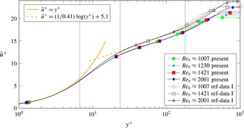
Mean velocity profiles with wall scaling. As references, the yellow lines indicate the law of the wall and the grey profiles show incompressible DNS results from Schlatter & Örlü (Reference Schlatter and Örlü2010). The coloured profiles show the present TBL data. The vertical, grey lines indicate locations for $Re_{\unicode[STIX]{x1D703}}\approx 1230$ at which data are plotted in the results section.

The data are obtained from a fully resolved DNS with an in-house compressible Navier–Stokes solver (Sandberg Reference Sandberg2015). The spatial discretisation is performed using fourth-order accurate standard differences in the streamwise and wall-normal directions, whereas the spanwise direction is discretised using a Fourier decomposition. For the discretisation of time a fourth-order accurate five-step Runge–Kutta method was chosen. Further details of the numerical methods are outlined in Bechlars (Reference Bechlars2015), Sandberg (Reference Sandberg2015). The grid is a structured Cartesian mesh and contains $7200\times 260$ points in the streamwise and wall-normal directions. In the spanwise direction, $193$ spanwise Fourier modes were used. This leads to a total of approximately $723$ million collocation points in the domain. The grid is stretched in the streamwise direction to keep the wall-scaled spacing relatively constant. The streamwise spacing has an upper bound of $\unicode[STIX]{x0394}x^{+}<5.12$ throughout the entire domain. The wall-normal location of the first point of the wall ( $y=0$ ) is located at $y^{+}|_{1}\approx 0.600{-}0.712$ and the tenth grid point is located at $y^{+}|_{10}\approx 5.43{-}6.40$ . The collocation points in the spanwise direction have a spacing of $\unicode[STIX]{x0394}z^{+}\approx 3.72{-}4.38$ . After an initial transient of the simulation the flow reaches a statistically steady state. All presented data are sampled in the statistically steady regime. The statistics in § 2 are sampled over a non-dimensional time period of $\unicode[STIX]{x0394}{\mathcal{T}}\approx 575(\unicode[STIX]{x1D6FF}_{99,in}/U_{\infty })$ with $U_{\infty }$ denoting the free stream velocity. The profiles of the mean streamwise velocity scaled with the friction velocity $u_{\unicode[STIX]{x1D749}}$ are presented in figure 1. The plot shows the incompressible law of the wall (in orange) as reference. Further, results of an incompressible DNS of a turbulent boundary layer (Schlatter & Örlü Reference Schlatter and Örlü2010) are added. The linear behaviour in the viscous sublayer as well as the slope of the logarithmic layer are captured well in the DNS of the present work. This is a first indication that the typical dynamics of a TBL is recovered in this simulation. The slight shift of the logarithmic layer and the wall-scaled maximum velocity reflect a deviation in skin friction. The reason for this is that we compare a compressible to an incompressible flow. The wall temperature in the present case is $1.05$ compared to the free stream. 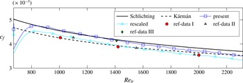This leads to an increase of viscosity due to Sutherland’s law towards the wall ( $\unicode[STIX]{x1D707}_{wall}=1.05$ ) which is directly affecting the skin friction at the wall. Figure 2 shows the development of the skin friction ( $c_{f}=2(\unicode[STIX]{x1D707}_{wall}/Re_{\infty })(\unicode[STIX]{x2202}\tilde{u} /\unicode[STIX]{x2202}y)$ ) in the present DNS in blue compared to different incompressible references. The skin friction of Spalart (Reference Spalart1988) (ref-data III) matches well, whereas the DNSs of Jiménez et al. (Reference Jiménez, Hoyas, Simens and Mizuno2010) (ref-data II) and Schlatter & Örlü (Reference Schlatter and Örlü2010) (ref-data I) are significantly lower. However, it can be shown by a simple scaling with the local wall viscosity, that this is a pure temperature effect. The cyan coloured line shows the skin friction divided by the local viscosity at the wall ( $c_{f,rescaled}=2(1/Re_{\infty })(\unicode[STIX]{x2202}\tilde{u} /\unicode[STIX]{x2202}y)$ ). The rescaled viscosity shows a perfect match with results of Jiménez et al. (Reference Jiménez, Hoyas, Simens and Mizuno2010), Schlatter & Örlü (Reference Schlatter and Örlü2010). This implies that the actual velocity gradient at the wall matches whereas the viscosity is different to the incompressible reference data which results in a difference of skin friction and, as we will see later, lower intensities of turbulence.

Figure 2.

The skin friction comparison shows the two incompressible empirical formulas of Schlichting (continuous) and Kármán–Schoenherr (dashed). The dots mark the values obtained by incompressible DNS from Schlatter & Örlü (Reference Schlatter and Örlü2010) (red), Jiménez et al. (Reference Jiménez, Hoyas, Simens and Mizuno2010) (grey) and Spalart (Reference Spalart1988) (green). The blue line shows the actual data of the present work, whereas the cyan line shows the present data after rescaling with the local wall viscosity.

Figure 3.

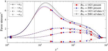
Comparison of the Favre stress tensor of the present work with the DNS results of Schlatter & Örlü (Reference Schlatter and Örlü2010). The vertical grey lines indicate locations at which data are plotted in the results section.

Figure 3 shows the distribution of turbulence in the boundary layer. The components of the Favre stress tensor $-\unicode[STIX]{x1D70E}$ are shown with wall scaling and plotted against the DNS data of Schlatter & Örlü (Reference Schlatter and Örlü2010). The development of the profiles match and the amplitudes are well in the range of differences seen in the literature (e.g. Spalart Reference Spalart1988; Jiménez et al. Reference Jiménez, Hoyas, Simens and Mizuno2010; Schlatter & Örlü Reference Schlatter and Örlü2010). The streamwise normal component $-\unicode[STIX]{x1D70E}_{11}$ shows a very good match in the viscous sublayer, but the data of the present work do not recover the full intensity of the streamwise fluctuations in the buffer layer. This is caused by the difference in skin friction mentioned before. The mismatch of the buffer layer decays in the logarithmic sublayer so that there is an excellent match in the outer layer. On the other hand, all other components of the Favre stress tensor $-\unicode[STIX]{x1D70E}$ show a very good match with the reference data throughout the entire wall-normal direction. Besides the wall-normal distribution, the streamwise development is predicted correctly as well. It can be seen that both, present data as well as reference data, show the same trend with increased Reynolds number.

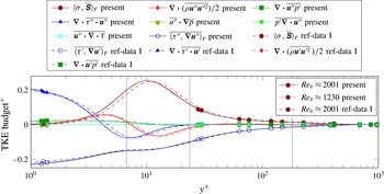
Figure 4 shows the mean budget of the turbulent kinetic energy $k$ . The figure compares the budget sampled from the data of the present work compared to the DNS data of Schlatter & Örlü (Reference Schlatter and Örlü2010). A very good agreement can be seen over the entire wall-normal direction. All amplitudes match almost perfectly and the differences are mainly due to shifts of the respective profiles in the wall-normal direction. The peak of turbulent production, for instance, is closer to the wall in the present dataset than it is for the incompressible DNS data of Schlatter & Örlü (Reference Schlatter and Örlü2010). On the other hand, the magnitude of dissipation and diffusion at the wall are slightly increased. Both can be explained by the above argument that in the present compressible flow the wall-normal gradient of the mean streamwise velocity component matches the incompressible gradients of Jiménez et al. (Reference Jiménez, Hoyas, Simens and Mizuno2010), Schlatter & Örlü (Reference Schlatter and Örlü2010), but the viscosity is higher and therefore the diffusion at the wall is increased. Either way, all differences are well within an acceptable range and the data are therefore seen as well suited for a detailed study of the variation of the strain–rotation relation and enstrophy production in a TBL.

Figure 4.

Turbulent kinetic energy budget at $Re_{\unicode[STIX]{x1D703}}=1230$ and $Re_{\unicode[STIX]{x1D703}}=2001$ . Results of the present work are shown as continuous and dotted lines, respectively, and compared with results of Schlatter & Örlü (Reference Schlatter and Örlü2010) at $Re_{\unicode[STIX]{x1D703}}=2001$ (dashed lines). The vertical grey lines indicate locations at which data are plotted in the results section.

The data for the following investigations were obtained in a volume that reaches from $Re_{\unicode[STIX]{x1D703}}\approx 1224{-}1248$ ( $Re_{\unicode[STIX]{x1D749}}\approx 481{-}491$ ) in the streamwise direction, covers approximately $120\,\%$ of the local boundary layer thickness $\unicode[STIX]{x1D6FF}_{99}(Re_{\unicode[STIX]{x1D703}}=1230)$ and covers the full spanwise extent of the domain. The sample volume has a sufficiently short streamwise direction such that statistical homogeneity can be assumed over its streamwise extent as well as in the spanwise direction. The statistics in §§ 3 and 4 is sampled over a non-dimensional time period of $\unicode[STIX]{x0394}{\mathcal{T}}\approx 90.4(\unicode[STIX]{x1D6FF}_{99}(Re_{\unicode[STIX]{x1D703}}=1230)/U_{\infty })$ with $\unicode[STIX]{x1D6FF}_{99}(Re_{\unicode[STIX]{x1D703}}=1230)$ denoting the boundary layer thickness defined as the wall distance when the mean streamwise velocity component reaches $99\,\%$ of the free stream velocity at the downstream location $Re_{\unicode[STIX]{x1D703}}=1230$ .

In figures 1 and 4 the vertical lines mark the wall-normal locations that are chosen for more detailed analysis in §§ 3 and 4. Overall, it can be stated that the wall-normal gradient of the mean streamwise velocity component and other quantities vary strongly over the wall-normal location, These gradients are the driving force of turbulence in this particular flow and the effect of their wall-normal variation are investigated in the next section.

3 Wall-normal development of enstrophy production

As a reflection of vortex stretching and vortex contraction, and therefore a representation of the cascading mechanism of kinetic energy in a turbulent flow, the highest values of enstrophy production are expected in the near-wall region. Figure 5(a) shows the development of the mean production in the wall-normal direction of the turbulent boundary layer. The components of the velocity gradient tensor $\unicode[STIX]{x1D63C}$ are scaled with the free stream velocity $U_{e}$ and the boundary layer thickness $\unicode[STIX]{x1D6FF}_{99}$ to $\breve{\unicode[STIX]{x1D63C}}=\unicode[STIX]{x1D63C}\unicode[STIX]{x1D6FF}_{99}/U_{e}$ . Unlike the production of turbulent kinetic energy (figure 4), the enstrophy production does not peak at $y^{+}\approx 10$ , but it reaches its maximum value closer to the wall. Wang & Lu (Reference Wang and Lu2012) showed that in a supersonic boundary layer the global maximum is located in the viscous sublayer at $y^{+}\approx 4$ . Above $y^{+}\geqslant 6.7$ the mean enstrophy production develops an exponential decrease with increasing distance to the wall and remains positive throughout the entire boundary layer. Figure 5(a) shows that the pressure–diffusion term of the enstrophy dynamics (1.2) increases towards the wall as well. This indicates that viscosity and pressure effects become stronger towards the wall. In contrast to the case of the turbulent kinetic energy (figure 4), viscosity effects do not become the dominant contributors for the enstrophy dynamics. Hence, the enstrophy production remains the dominant term in the dynamics throughout the entire boundary layer.

Figure 5.

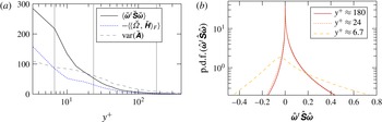
Overview of enstrophy production in the turbulent boundary layer flow. (a) Wall-normal development of the mean enstrophy production, enstrophy pressure–diffusion term and the variance of the velocity gradient tensor in the outer scaling ( $\breve{f}=f(\unicode[STIX]{x1D6FF}_{99}/U_{e})$ ). Grey vertical lines indicate the location at which the p.d.f.s (b) are taken. (b) P.d.f. of the scaled enstrophy production at three different wall-normal locations.

In contrast to the strictly positive net production, the p.d.f.s (figure 5 b) reveal that the instantaneous production has significant negative contributions. For this plot and for the following we introduce a scaling based on the local variance of the velocity gradient tensor magnitude

where $\langle \bullet \rangle$ denotes the temporal mean. The development of the variance over the wall-normal direction is shown in figure 5(a) to obtain the relation between the scaled quantities at different locations. The velocity gradient tensor quantities are scaled as

For $y^{+}\approx 24$ and $y^{+}\approx 180$ a significant peak can be seen at zero while an asymmetric shape of the p.d.f. is developed. The legs towards positive production reach to significantly higher magnitudes and are fatter than the ones on the negative side. This underlines the general consensus found in the literature (e.g. Taylor Reference Taylor1938; Tennekes & Lumley Reference Tennekes and Lumley1972) that vortex stretching (positive enstrophy production) is favoured over vortex compression (negative enstrophy production). Further, the shapes of the p.d.f.s agree well with experimental results of turbulent shear flow and turbulent jet results from Mullin & Dahm (Reference Mullin and Dahm2006), Buxton & Ganapathisubramani (Reference Buxton and Ganapathisubramani2010), respectively. Above $y^{+}\approx 24$ the enstrophy production does not change its character – therefore all scaled p.d.f. collapse for higher regions. Further, the most likely value stays at zero and its variance scales well with the variance of the velocity gradient tensor magnitude $\text{var}(\unicode[STIX]{x1D74E}^{t}\unicode[STIX]{x1D64E}\unicode[STIX]{x1D74E})\sim \text{var}(\unicode[STIX]{x1D63C})^{3}$ . However, closer to the wall the properties of the p.d.f. changes. The variance of the production no longer scales linearly with the velocity gradient tensor magnitude variance and is much higher than at the higher locations in a relative sense. Both the negative and positive tails of the p.d.f. are increasing in size. However, additional to the negative shift of the peak, the negative tail is growing comparatively more than the positive one.

Figure 6.

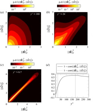
Joint p.d.f. of normalised strain rate magnitude squared and normalised rotation magnitude squared at three different wall-normal locations (a–c). The development of correlations between strain rate and rotation rate in the wall-normal direction (d).

To understand these changes in the near-wall region the enstrophy production is decomposed based on the eigen-decomposition of the strain rate tensor (1.4). In this identity we see that the scaling term for the production is $\Vert \unicode[STIX]{x1D6FA}\Vert _{F}^{2}\Vert \unicode[STIX]{x1D64E}\Vert _{F}$ . To investigate how these strain and rotation tensor magnitudes are coupled we study the joint p.d.f. of $\Vert \unicode[STIX]{x1D6FA}\Vert _{F}^{2}$ and $\Vert \unicode[STIX]{x1D64E}\Vert _{F}^{2}$ (figure 6 a–c). The joint p.d.f.s strongly agree with results presented by Blackburn et al. (Reference Blackburn, Mansour and Cantwell1996), Chong et al. (Reference Chong, Soria, Perry, Chacin, Cantwell and Na1998). According to the interpretation of Perry & Chong (Reference Perry and Chong1994) (see introduction) the predominant structure type in the near-wall region are vortex sheets (figure 6 c). Thus, what we can conclude from these plots is that vorticity is strongly coupled to the strain rate which implies (Tsinober Reference Tsinober2000) that vortices in this region of the boundary layer have a relatively strong dissipative character. However, moving further away from the wall this dominance of vortex sheets is replaced by a mix of vortex sheets, vortex tubes and non-swirling, straining structures, which agrees with the results of Chong et al. (Reference Chong, Soria, Perry, Chacin, Cantwell and Na1998). In the upper buffer layer region (figure 6 b) we find a weaker coupling for smaller velocity gradient tensor magnitudes ( $\Vert \unicode[STIX]{x1D63C}\Vert _{F}^{2}=\Vert \unicode[STIX]{x1D64E}\Vert _{F}^{2}+\Vert \unicode[STIX]{x1D6FA}\Vert _{F}^{2}$ ), but the strong coupling of strain and rotation tensor magnitude is still present for large gradients. Above the buffer layer (figure 6 a – representative for all higher locations) the strong coupling is lost for any velocity gradient tensor magnitude. For the scaling term $\Vert \unicode[STIX]{x1D6FA}\Vert _{F}^{2}\Vert \unicode[STIX]{x1D64E}\Vert _{F}$ of the enstrophy production the correlation of the strain rate magnitude and the rotation rate magnitude squared is an essential quantity. A strong correlation increases the likelihood of relatively large values of the term

The correlation $\text{corr}(\Vert \unicode[STIX]{x1D64E}\Vert _{F},\Vert \unicode[STIX]{x1D6FA}\Vert _{F}^{2})$ is shown in figure 6(d) together with the correlation $\text{corr}(\Vert \unicode[STIX]{x1D64E}\Vert _{F}^{2},\Vert \unicode[STIX]{x1D6FA}\Vert _{F}^{2})$ to illustrate why a coupling of $\Vert \unicode[STIX]{x1D64E}\Vert _{F}$ and $\Vert \unicode[STIX]{x1D6FA}\Vert _{F}^{2}$ is closely related to a coupling of $\Vert \unicode[STIX]{x1D64E}\Vert _{F}^{2}$ and $\Vert \unicode[STIX]{x1D6FA}\Vert _{F}^{2}$ . The increasing correlation in the near-wall region could be caused by a more dense packing of vortices at the wall – a feature that will be discussed later. This causes an increased interaction of their strain fields which acts in addition to the interaction of the strain fields with the wall itself. The enhanced interaction then amplifies the correlation between strain and rotation. This would agree with the idea of vortex sheets discussed before. Another idea is that a single shear component of the velocity gradient tensor becomes much stronger than all the other components when approaching the wall. This would lead to the strain rate and rotation rate tensor magnitudes coming closer to each other relative to the velocity gradient tensor magnitude. Hence we show that the difference $\unicode[STIX]{x1D700}$ between the relative magnitudes becomes small for a dominant shear component. Therefore we have

with the normalised velocity gradient components

A specific $a_{ij}$ can be defined as dominant over others if its normalised component shows a tendency to approach unity.

It can be shown that all other normalised components tend to zero. If an off-diagonal ( $m\neq l$ ) component of the velocity gradient tensor becomes dominant then the difference $\unicode[STIX]{x1D700}$ becomes small as a consequence of (3.6):

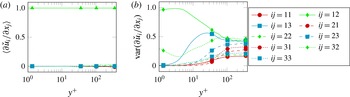
That this is the case in the near-wall region of the present TBL is shown in figure 7. The dominance of the wall-normal derivative of the streamwise velocity component is given in the entire TBL as shown in 7(a). The normalised variance of the same velocity gradient component shows that also the fluctuations become dominant in the near-wall region. Therefore $\unicode[STIX]{x1D64E}$ and $\unicode[STIX]{x1D6FA}$ have a similar magnitude in the near-wall region. Hence, the increased correlation of their magnitudes in the near-wall region can be explained by the dominance of a single shear component.

Figure 7.

Wall-normal development of the mean (a) and variance (b) of the normalised velocity gradient components ( $\check{f}=f/\Vert \unicode[STIX]{x1D63C}\Vert _{F}$ ).

Figure 8.

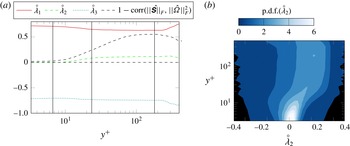
Wall-normal development of the normalised strain rates in the turbulent boundary layer. (a) Mean development of the principal strain rates. The dashed black line shows the correlation of $\Vert \unicode[STIX]{x1D64E}\Vert _{F}^{2}$ and $\Vert \unicode[STIX]{x1D6FA}\Vert _{F}^{2}$ . The dashed grey line marks zero. (b) Wall-normal development of the normalised strain rates in the turbulent boundary layer.

The magnitudes, imposed by the strain rate and the rotation rate, are scaled by the combination of the relative principal strain rates and the alignments between the vorticity vector and the respective principal strain direction (1.5). The mean development of the principal strain rates are shown in figure 8. In the outer layer as well as in the logarithmic layer we find a slightly positive value for the mean of the intermediate strain. This, qualitatively, agrees with literature about HIT (Ashurst et al. Reference Ashurst, Kerstein, Kerr and Gibson1987) and weak shear layers (e.g. Ganapathisubramani et al. Reference Ganapathisubramani, Lakshminarasimhan and Clemens2008). However, a quantitative comparison reveals a disagreement with the ratio of $(\unicode[STIX]{x1D706}_{1}:\unicode[STIX]{x1D706}_{2}:\unicode[STIX]{x1D706}_{3})$ in the approximate range $(2.5:1:-3.5)$ to $(3.5:1:-4.5)$ that were previously published. In case of the present TBL we obtain the ratios $(5.5:1:-6.5)$ for $y^{+}\approx 180$ , $(7.8:1:-8.8)$ for $y^{+}\approx 24$ and $(128:-1:-127)$ for $y^{+}\approx 6.7$ . Therefore the plots show that when approaching the wall, the relative intermediate strain tends to zero. It is slightly negative in the near-wall region, but its magnitude is small enough that the sign does not play a significant role. The p.d.f.s in figure 8(b) show that the fluctuations around this zero mean are relatively small compared to the fluctuations that can be found in the outer layer. Further, the p.d.f. is skewed towards positive values in the higher regions of the boundary layer, an observation that does not hold for the near-wall region. In the near-wall region we find a nearly symmetric p.d.f.

If we assume that a turbulent flow can be described by vortices and their interactions, then a modified vortex stretch model introduced by Ashurst et al. (Reference Ashurst, Kerstein, Kerr and Gibson1987) can be used to interpret the development of the principal strains in the boundary layer. In the model a vortex is described as a line vortex that stretches along its axis. The stretching mechanism itself creates a strain field with the according principal strain ratio described by $R_{stretch}:=(-1:2:-1)$ . However, the vortex’s own strain field, caused by the rotation that decays with increasing distance to the axis, causes a shear that results in a principal strain ratio described by $R_{os}:=(1:0:-1)$ . Depending on the ratio of the strength of the stretching to the strength of the shearing due to the vortex rotation $(\unicode[STIX]{x1D6FE}_{stretch}:\unicode[STIX]{x1D6FE}_{os})$ this can be expressed as the combined ratio $\unicode[STIX]{x1D6FE}_{stretch}R_{stretch}+\unicode[STIX]{x1D6FE}_{os}R_{os}$ . Ashurst et al. (Reference Ashurst, Kerstein, Kerr and Gibson1987) found that a ratio $(\unicode[STIX]{x1D6FE}_{stretch}:\unicode[STIX]{x1D6FE}_{os})=(1:7)$ leads to the ratio $(\unicode[STIX]{x1D706}_{1}:\unicode[STIX]{x1D706}_{2}:\unicode[STIX]{x1D706}_{3})=(3:1:-4)$ that fits well to the ratio of principal strains found for HIT and weak shear layers as mentioned before. However, in the current TBL study these flows we find a very strong anisotropic velocity gradient field, especially in the near-wall region, which is reflected by the strong wall-normal gradient of the streamwise velocity component. Therefore we suggest the addition of a ratio for the background strain $R_{bgs}$ to the vortex stretch model. This ratio depends on the alignment of the background strain with the background rotation. The alignment that we find in the mean flow suggests that the background strain in the form of the mean strain of the TBL is orthogonal to the mean vorticity vector. Therefore the ratio of the background strain will act in the same way as the strain caused by the vortex’s own strain field $R_{bgs}:=(1:0:-1)$ . The suggested ratio described by the extended model would then be $\unicode[STIX]{x1D6FE}_{stretch}R_{stretch}+\unicode[STIX]{x1D6FE}_{os}R_{os}+\unicode[STIX]{x1D6FE}_{bgs}R_{bgs}$ . For the TBL the last two components can be summarised as $\unicode[STIX]{x1D6FE}_{shear}:=0.5(\unicode[STIX]{x1D6FE}_{os}+\unicode[STIX]{x1D6FE}_{bgs})$ and $R_{shear}:=0.5(R_{os}+R_{bgs})$ . This reduces the generalised model to $\unicode[STIX]{x1D6FE}_{stretch}R_{stretch}+\unicode[STIX]{x1D6FE}_{strain}R_{strain}$ . Contrasting the HIT and weak shear layer results we have found a strong increase of correlation between strain rate and rotation rate when approaching the wall. We believe that this variation together with the background strain strongly influences the ratio $(\unicode[STIX]{x1D6FE}_{stretch}:\unicode[STIX]{x1D6FE}_{shear})$ and drives it to the even more extreme values presented above.

Figure 9.

Top view onto a boundary layer. The instantaneous snapshots of the $\unicode[STIX]{x1D706}_{ci}$ -criterion are taken at the same instance of time at two different heights in the boundary layer. The right is a location within the logarithmic layer ( $y^{+}\approx 114$ , b) and the left shows a location at the lower part of the buffer layer ( $y^{+}\approx 11$ , a). The flow direction is bottom to top.

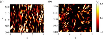
Overall, its seems that at the wall, because of its strain field, turbulence develops a strong variation in two directions whereas the third direction is nearly homogeneous as implied by the nearly vanishing relative intermediate strain. The background strain associated with the mean flow acts only in two directions due to the spanwise statistical homogeneity of the TBL. This also appears to hold for the instantaneous turbulent structures at the wall (figure 9). We find relatively long streamwise elongated densely packed structures in the near-wall region (figure 9 a), whereas the structures in higher layers are more randomly aligned and less densely packed (figure 9 b). When the structures are densely packed at the wall, then their strain fields amplify each other, which leads to strong strain fields produced by the vortices themselves.

Figure 10.

P.d.f.s of the alignment between the vorticity vector and the principal strain directions at three different wall-normal locations. (a) $y^{+}\approx 180$ , (b) $y^{+}\approx 24$ , (c) $y^{+}\approx 6.7$ .

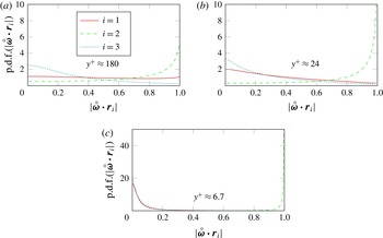
Besides the principal strains, the other part of the term (1.5) that weights the strain rate magnitude and the rotation magnitude in the enstrophy production (1.4) is the alignment of the vorticity vector with the principal strain directions. In figure 10 these alignments are shown for different wall-normal locations in the TBL. For the outer most location ( $y^{+}\approx 180$ ) the alignments agree well with the ones stated for HIT and weak shear layers in literature (e.g. Ashurst et al. Reference Ashurst, Kerstein, Kerr and Gibson1987; Ganapathisubramani et al. Reference Ganapathisubramani, Lakshminarasimhan and Clemens2008; Hamlington et al. Reference Hamlington, Schumacher and Dahm2008; Meneveau Reference Meneveau2011; Leung et al. Reference Leung, Swaminathan and Davidson2012). Vorticity shows an arbitrary alignment with the extensive strain direction ( $i=1$ ), but tends to align in parallel with the intermediate strain direction ( $i=2$ ). The tendency to an orthogonal alignment between the vorticity vector and the compressive strain direction ( $i=3$ ) can be observed. Ashurst et al. (Reference Ashurst, Kerstein, Kerr and Gibson1987) proposed with their previously described vortex stretch model that this alignment reflects the alignment of the vorticity vector with the vortex induced strain field rather than the alignment of a vortex with the imposed strain field of other structures and/or boundary conditions. This is supported by the work of Hamlington et al. (Reference Hamlington, Schumacher and Dahm2008) and Leung et al. (Reference Leung, Swaminathan and Davidson2012) as discussed in the introduction.

The change of the alignments with the wall-normal location shown in figure 10 agrees well with the variations that where found by Blackburn et al. (Reference Blackburn, Mansour and Cantwell1996). The parallel alignment of vorticity with the intermediate strain direction becomes more likely when approaching the wall. At the same time the orthogonal alignment with the compressive strain direction further increases its frequency of occurrence. Further, the arbitrary alignment of vorticity and the extensive strain direction does not hold anymore when approaching the wall. Already at $y^{+}\approx 24$ we find a weak trend of an orthogonal alignment between vorticity and the extensive strain direction. At $y^{+}\approx 6.7$ the tendency of this orthogonal alignment becomes strong enough to show the same p.d.f. as $|\unicode[STIX]{x1D74E}\boldsymbol{\cdot }\boldsymbol{r}_{3}|$ .

As we have seen when discussing the principal strains, the strain field of the vortices is dominated by the strain field that is induced by the vortex’s own shear rather than the stretching strain. However, the vortex’s rotation axis is aligned with the stretching strain direction and therefore we find $|\unicode[STIX]{x1D74E}\boldsymbol{\cdot }\boldsymbol{r}_{2}|\rightarrow 1$ . On the other hand, the surrounding strain field develops an alignment with the axis normal plane which leads to $|\unicode[STIX]{x1D74E}\boldsymbol{\cdot }\boldsymbol{r}_{1}|\rightarrow 0$ and $|\unicode[STIX]{x1D74E}\boldsymbol{\cdot }\boldsymbol{r}_{3}|\rightarrow 0$ .

Figure 11.

Mean alignment of vorticity with the three principal strain directions (continuous lines). Correlation coefficient between the strain rate magnitude squared and the rotation rate magnitude squared (dashed line).

Figure 12.

Intermittency measure $\unicode[STIX]{x1D6E4}_{\unicode[STIX]{x0394}{\mathcal{T}}}$ plotted over wall distance $y^{+}$ . The filter time scales are $\unicode[STIX]{x0394}{\mathcal{T}}^{+}\approx 10$ and $\unicode[STIX]{x0394}\breve{{\mathcal{T}}}=\unicode[STIX]{x1D6FF}_{99}/U_{e}\approx 1$ .

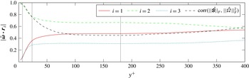
In figure 11 the development of the mean alignment of the vorticity vector with the principal strain directions is shown over the distance to the wall. Over a large part of the boundary layer we find a relatively constant mean alignment which coincides with the previously discussed results about HIT and weak shear layers. We find a slight variation towards the far outer region. 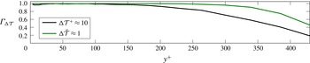Similarly we see a variation of the ratio of the mean principal strains in the far outer layer after developing a plateau in the logarithmic layer and the beginning of the outer layer (figure 8 a). Both are believed to be caused by sparse turbulent spots for which the interaction with other structures exhibits a lag. Therefore a measure of intermittency, $\unicode[STIX]{x1D6E4}_{\unicode[STIX]{x0394}{\mathcal{T}}}$ , is shown for two different parameters in figure 12. For the intermittency measures we define a temporal box filter for the streamwise velocity component

with the box width $\unicode[STIX]{x0394}{\mathcal{T}}$ . This is applied to a turbulent/non-turbulent indicator function that detects if the variation of filtered and unfiltered velocity signals is larger than one per cent of the local Reynolds-averaged streamwise velocity

The intermittency measure is then defined as the Reynolds average of the indicator function $\unicode[STIX]{x1D6E4}_{\unicode[STIX]{x0394}{\mathcal{T}}}:=\langle \unicode[STIX]{x1D6FE}\rangle$ . A value of unity can thus be seen as a measure for a fully turbulent signal whereas zero states a laminar signal. For the plot we choose a measure based on outer time scales as well as one based on inner time scales. Both indicate that turbulence occurs as rare events in the outer layer compared to the region below. This affects the outer region results in terms of alignment and strain composition. However, the stronger change of the alignments can be seen in the near-wall region as discussed in the previous paragraph. The mean alignment of vorticity with the intermediate strain direction becomes parallel whereas vorticity aligns perpendicular with the remaining two principal strain directions. Note that the results for the outer boundary layer have not been conditioned with respect to intermittency and thus the alignments start to change below $y^{+}\lesssim 110$ which is roughly the region where the correlation of strain rate magnitude and rotation rate magnitude starts to vary.

4 Characteristic decomposition of enstrophy production

In the previous section the enstrophy production was studied by considering an eigenvalue decomposition of the strain rate tensor (1.4). We have seen how certain parts of the production vary with the distance to the wall and how some of them are coupled. In their work on the experimental data of the far field of a turbulent jet, Buxton & Ganapathisubramani (Reference Buxton and Ganapathisubramani2010) showed that the sign of the production, i.e. whether enstrophy is produced or destroyed, is dictated by the alignment of vorticity with the extensive strain direction. Applying a characteristic decomposition to the turbulent flow, the dominant enstrophy destroying structures were found within the unstable/contracting vortical structures. In this work we discuss to what extent this holds in a turbulent boundary layer. A prerequisite for this is the discussion of the distribution of the characteristic structure types in the turbulent boundary layer.

The applied characteristic decomposition is based on the critical point concept first introduced by Perry & Chong (Reference Perry and Chong1987) which decomposes a flow according to the form of the eigenvalues of the local velocity gradient tensor. Therefore this analysis is purely local and describes the character of a structure at the location of the current fluid particle only. It does not describe the character of a structure as a whole. A better overview of the method is provided in the original publication of Perry & Chong (Reference Perry and Chong1987) or the summary about Lagrangian dynamics by Meneveau (Reference Meneveau2011). The method distinguishes between different characteristic local flow topologies depending on the first three velocity gradient invariants $P,Q$ and $R$ . These invariants span a state space, the $PQR$ -space, in which we find certain regions defining certain properties of the eigenvalues, and therefore certain properties of the local flow topology at the fluid particle. $P$ , which is the additive inverse of the dilatation $-\unicode[STIX]{x1D735}\boldsymbol{\cdot }\boldsymbol{u}$ , is zero for incompressible flows. For compressible cases $P$ is not necessarily zero. However, for our results at a Mach number of $M_{\infty }=0.5$ we find no significant dependency of the results on $P$ . This is confirmed by figure 13(a–c) where the isolines enclosing $95\,\%$ of the joint p.d.f. of $Q$ and $R$ were conditioned for relatively strong compression and decompression events. This resulted in only minor deviations which become even less significant the lower the enclosed probability is chosen (not shown here). Therefore we map the results obtained from the compressible analysis onto the subset of the $PQR$ -space defined by $P=0$ , this we call $QR$ -space. The distinction of characteristic topologies is made in analogy to the incompressible case as explained in Perry & Chong (Reference Perry and Chong1987), Chong, Perry & Cantwell (Reference Chong, Perry and Cantwell1990), Soria et al. (Reference Soria, Sondergaard, Cantwell, Chong and Perry1994), Ooi et al. (Reference Ooi, Martin, Soria and Chong1999) and Bechlars (Reference Bechlars2015) and summarised in the following. The $QR$ -space is spanned by the second and third invariant, $Q$ and $R$ , of the velocity gradient tensor. From the point of view of a fluid particle located on a structure, it allows the distinction between four different states of the structure at the location of the particle. A schematic description of the $QR$ -space and the four structure types can be found in, e.g. Ooi et al. (Reference Ooi, Martin, Soria and Chong1999). The discriminant of the velocity gradient tensor $\unicode[STIX]{x1D6E5}$ has an important role in this decomposition. For positive values of $\unicode[STIX]{x1D6E5}>0$ the velocity gradient tensor has one purely real eigenvalue and a complex conjugate pair of complex eigenvalues and therefore the fluid particle sits on a part of a structure that has a rotational character. On the other hand, if $\unicode[STIX]{x1D6E5}\leqslant 0$ , then all eigenvalues of the velocity gradient tensor are purely real and the supporting structure is non-swirling and straining at the location of the fluid particle. Further, for negative values of the third invariant $R\leqslant 0$ we find two contracting directions and one stretching direction, whereas if $R$ is positive we find two stretching direction and one contraction direction of the structure at the location of the fluid particle. So four characteristic structure types can be described by vortical structure with stretching character $\unicode[STIX]{x1D6E5}>0$ ; $R\leqslant 0$ (I); vortical structure with contracting character $\unicode[STIX]{x1D6E5}>0$ ; $R>0$ (II); non-swirling, straining structure with flattening character $\unicode[STIX]{x1D6E5}\leqslant 0$ ; $R>0$ (III); and non-swirling, straining structure with elongating character $\unicode[STIX]{x1D6E5}\leqslant 0$ ; $R\leqslant 0$ (IV).

Figure 13.

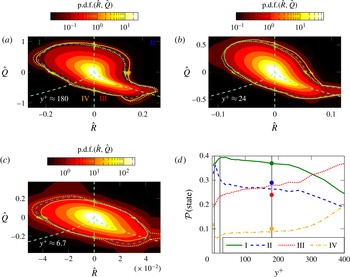
(a–c) Joint p.d.f.s of the normalised second ( $\hat{Q}$ ) and third ( $\hat{R}$ ) invariant of the velocity gradient tensor at three different locations in the boundary layer. The blue line in the p.d.f. is the isoline that encloses $95\,\%$ of all events. The red and green line in the p.d.f. is the isoline that encloses $95\,\%$ of all events conditioned for compression ( $P\geqslant \unicode[STIX]{x1D6FC}\unicode[STIX]{x1D70E}(P)$ ) and decompression ( $P\leqslant -\unicode[STIX]{x1D6FC}\unicode[STIX]{x1D70E}(P)$ ) events. Here $\unicode[STIX]{x1D70E}(P)$ is the local standard deviation of $P$ and $\unicode[STIX]{x1D6FC}$ is a factor ((a) $\unicode[STIX]{x1D6FC}\approx 2.0$ , (b) $\unicode[STIX]{x1D6FC}\approx 1.3$ , (c) $\unicode[STIX]{x1D6FC}\approx 1.1$ ). (a) $y^{+}\approx 180$ , (b) $y^{+}\approx 24$ , (c) $y^{+}\approx 6.7$ . (d) Frequency of occurrence ${\mathcal{P}}$ (state) of the respective characteristic states over the wall-normal direction. The vertical grey lines indicate the locations where samples are taken for a more detailed analysis. The coloured dots mark the respective distributions obtained in the far field of a turbulent jet (Buxton & Ganapathisubramani Reference Buxton and Ganapathisubramani2010).

According to the previous normalisation of the different parts of the velocity gradient tensor (3.1) the second and third invariants of the velocity gradient tensor are normalised using the variance of the velocity gradient tensor (3.2)

The frequency of occurrence of the characteristic structures in a flow can now be measured by sampling joint p.d.f.s of $R$ and $Q$ in the flow. The resulting plots were first shown by Vieillefosse (Reference Vieillefosse1982, Reference Vieillefosse1984) and are commonly known as $QR$ -plots and are shown for the present turbulent boundary layer in figure 13(a–c). All shown $QR$ -plots agree with literature. The shape of the plot of the outermost location at $y^{+}\approx 180$ (a) agrees in a wider sense with literature about HIT (Martin et al. Reference Martin, Ooi, Chong and Soria1998), the far field of a turbulent jet (Ganapathisubramani et al. Reference Ganapathisubramani, Lakshminarasimhan and Clemens2008) and experimental results of the outer layer of a turbulent boundary layer (Elsinga & Marusic Reference Elsinga and Marusic2010). In the buffer layer (figure 13 b) we find that the tail towards high values of $R$ and low values of $Q$ shrinks compared to the location further away from the wall. Furthermore, the teardrop shape appears to be more tilted counter-clockwise. At the location closest to the wall, at $y^{+}\approx 6.7$ (figure 13 c), the teardrop shows a nearly oval shape and becomes even more tilted counter-clockwise compared to both locations with larger values of $y^{+}$ . These results agree with the results Blackburn et al. (Reference Blackburn, Mansour and Cantwell1996) and Chong et al. (Reference Chong, Soria, Perry, Chacin, Cantwell and Na1998) show for different wall-normal locations in a turbulent boundary layer flow.

Reducing the complexity of the $QR$ -plots is possible by integrating the joint p.d.f. over the area of the respective characteristic types in the $QR$ -space. This leads to the probability ${\mathcal{P}}(\text{state})$ of each characteristic state I, II, III or IV. In the plot of these probabilities over the distance to the wall (figure 13 d) we see that even in the outer region there are strong variations of the characteristic distribution of turbulence. The coloured dots in figure 13(d) indicate the ratios that Buxton & Ganapathisubramani (Reference Buxton and Ganapathisubramani2010) stated for the far field of a jet flow. The data agree with the results of a supersonic TBL (Wang & Lu Reference Wang and Lu2012) conditioned for small values of $|\unicode[STIX]{x1D617}|$ . This, together with the previous conditioning of the joint p.d.f.s, shows that topological results affected by different levels of compressibility strength can be compared for small values of the first invariant of the velocity gradient tensor, $\unicode[STIX]{x1D617}$ . In general the relatively smooth changes in the outer layers are contrasted by the strong changes in the near-wall region. Especially the unstable/contracting vortical structures (II) have a relatively strong near-wall peak. Also the stable node/saddle structures (IV) show a considerable increase in their frequency of occurrence right at the wall. Here we discuss the effects the varying distribution of characteristic structures have on the enstrophy production. The other two structure types (I and III) have a slightly decreasing frequency of occurrence in the near-wall region when approaching the wall.

Figure 14.

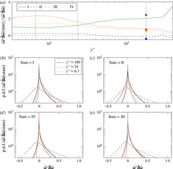
(a) Conditional average of the relative enstrophy production conditioned with the respective characteristic state plotted over the distance to the wall. The vertical grey lines indicate the locations where samples are taken for a more detailed analysis. The coloured dots mark the respective conditional averages obtained in the far field of a turbulent jet (Buxton & Ganapathisubramani Reference Buxton and Ganapathisubramani2010). (b–e) Conditional p.d.f.s of the relative enstrophy production conditioned with the respective characteristic state ((b) state $=$ I, (c) state $=$ II, (d) state $=$ IV, (e) state $=$ III) plotted at three different wall-normal locations. The grey lines show the unconditional p.d.f.s as reference.

The average production conditioned with the respective characteristic states is plotted over the wall-normal distance normalised by the unconditioned mean production (figure 14 a). Although there is a good qualitative agreement, we find that at no point do they match quantitatively the conditional production of the jet results by Buxton & Ganapathisubramani (Reference Buxton and Ganapathisubramani2010) that are marked as coloured dots in the plot. This is not very surprising as we have already seen in the previous section that the production is composed in a different way in the TBL than it is in the far field of the jet flow. Accordingly, we find a variation of the contribution of each characteristic structure type to the local enstrophy production. In the higher regions above $y^{+}\gtrsim 32$ the strongest enstrophy producers are vortices with stretching character. Additionally, in the region above $y^{+}\gtrsim 32$ the relative production of the two non-swirling, straining structure types is roughly half as strong as the relative production of the stretching vortices. This supports the idea that enstrophy production is strongly correlated with vortex stretching. The dominance of the relative production of stretching vortices becomes even stronger in the far outer region of the TBL. Further, the unstable/contracting vortical structures have a negative mean contribution to the enstrophy production above $y^{+}\gtrsim 60$ . On average these structures destroy enstrophy in the outer region which potentially indicates a backscatter mechanism in which the kinetic energy is transferred from smaller scales towards larger scales of motion. Whereas all the relative production terms are relatively constant in the logarithmic layer of the TBL, the variation becomes stronger in the near-wall region below $y^{+}\lesssim 40{-}50$ . We find a relative decrease of the relative production of stretching vortices which coincides with a relative increase of the relative production for non-swirling, straining, stable node/saddle structures as well as of unstable/contracting vortical structures. The latter even develop a positive contribution in the near-wall region. However, the strongest increase of relative production is caused by non-swirling, straining, unstable node/saddle structures. They become and stay the most dominant structures (with respect to relative production) below $y^{+}\lesssim 32$ . Overall we find that in the near-wall region non-swirling, straining structures become stronger producers of enstrophy than rotational structures. This supports the idea that the shear layers between the densely packed and ordered structures together with the background strain and background rotation become more dominant in producing enstrophy than vortex stretching in the near-wall region.

In analogy to the unconditional overall production (figure 5) we want to get an impression of the overall production for the respective structure types and its distribution across the structure types in the TBL. The p.d.f.s conditioned with the respective structure types at three selected locations (figure 14 b–e) allow more insight into the enstrophy production mechanism. Conditioned with the characteristic structure types the scaled p.d.f.s above $y^{+}\approx 24$ do not collapse perfectly anymore. Although they start to lose their self-similar character, they still show the same trends for the same conditions. The p.d.f.s of enstrophy production conditioned for the stable vortical structures (I) show an enlargement of their positive legs compared to the unconditional production in the region $y^{+}\gtrsim 24$ . For all other conditions the positive legs shorten or are nearly unaffected by the condition in this region. In the near-wall region we find different behaviours. The unstable straining structures (III) show a strong increase of the positive leg of the p.d.f. of enstrophy production. Further, the p.d.f. conditioned for the stable straining structures (IV) develops a thin and long positive leg. For the rotational structures (I, II) we find a smaller positive leg or no change of the positive leg of the p.d.f. in the near-wall region. Putting the picture together we find that in the region $y^{+}\gtrsim 24$ the stable vortices (I) are the dominant enstrophy producers through relatively strong, and relatively rare events, based on their skewed conditional p.d.f. of enstrophy production. However, in the near-wall region the opposite is true and the p.d.f. conditioned with the non-swirling, straining structures (III, IV) become more skewed towards the negative side. This indicates that near the wall the non-swirling, straining structures become the dominant producers of enstrophy through even stronger rare events.

For structure types I, III and IV in the region $y^{+}\gtrsim 24$ all negative legs are shorter than in the unconditional case. At the wall this only holds for type III. On the other hand, the enstrophy production p.d.f.s of the unstable rotational structures (II) have larger legs towards the negative side. This means that in the entire TBL we find an increased number of enstrophy destroying events associated with the unstable vortical structures compared to the stable vortical structures and non-swirling, straining structures. In light of the scale transfer of turbulent kinetic energy these results suggest that the unstable vortical structures play a key role in the backscatter mechanism that transfers kinetic energy from smaller scales of motion to larger scales of motion.

Figure 15.

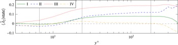
Conditional averages of the normalised intermediate strain conditioned with the respective characteristic state plotted over the wall-normal location. The vertical grey lines indicate the locations where samples are taken for a more detailed analysis.

The conditional mean development as well as the development of the conditional p.d.f.s of the normalised intermediate strain rate conditioned with the respective characteristic states are plotted in figure 15. The mean development shows similar behaviours for all conditions in the entire TBL, except for the far outer layer of the boundary layer where we find a strongly intermittent flow (figure 12). The mean intermediate strain rate is largest when conditioned with non-swirling, straining, unstable node/saddle structures (III) for which it is always positive. However, for the non-swirling, straining, stable node/saddle structures (IV) the intermediate strain is always around zero in the mean. For both rotational structure types (I and II) we find the mean intermediate strain rate is approximately half of the mean for characteristic type III in the logarithmic layer. Approaching the wall, both are decaying whereas the stable/stretching vortices level out around a zero intermediate strain rate and the unstable/contracting vortices level out around a slightly negative intermediate strain rate below $y^{+}\lesssim 10$ . We cannot draw further conclusions from the conditioned principal strain rates, but show this plot for completeness.

Figure 16.

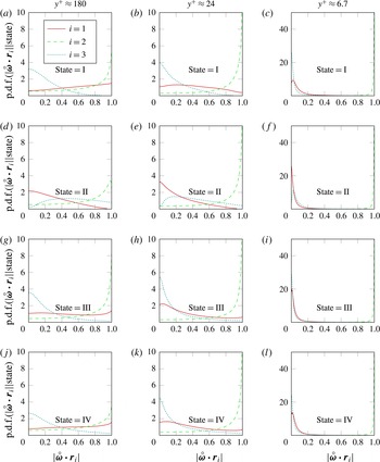
Conditional p.d.f.s of the alignment between the vorticity vector and the principal strain directions conditioned with the respective characteristic state ((a–c) state I, (d–f) state II, (g–i) state III, (j–l) state IV) at the wall-normal locations (columns) $y^{+}\approx 180$ (a,d,g,j), $y^{+}\approx 24$ (b,e,h,k) and $y^{+}\approx 6.7$ (c,f,i,l).

The remaining part of the weighting term in the conditioned enstrophy production is the conditioned alignment between vorticity vector and the principal strain directions. The results we found for $y^{+}\approx 180$ are shown in figure 16(a,d,g,j). The distributions of the alignments conditioned with the four characteristic states all agree qualitatively with the results for the alignment in the far field of a turbulent jet (Buxton & Ganapathisubramani Reference Buxton and Ganapathisubramani2010). The alignment of the extensive strain loses its overall arbitrary alignment with the vorticity vector. For stable vortices (I,a) we find both vectors developing a slight tendency to align in parallel. The same holds for the stable node/saddle structures (IV,j). Whereas the unstable node/saddle structures (III,g) still show an arbitrary alignment of $\unicode[STIX]{x1D74E}$ and $\boldsymbol{r}_{1}$ , we find a relatively strong perpendicular alignment of both for unstable vortical structures (II,d). The tendency of vorticity and intermediate strain direction to align in parallel is given for all structure types. However, the strength of this tendency does vary slightly between the different states. It is more pronounced for states I and III than it is for states II and IV. Moreover, for the unstable contracting vortices we find that the probability is high for both vectors to align nearly in parallel, but the p.d.f.s decrease in value just before reaching perfect alignment, where $|{\unicode[STIX]{x1D74E}\unicode[STIX]{x0030A}}\boldsymbol{\cdot }\boldsymbol{r}_{2}|=1$ . However, Buxton & Ganapathisubramani (Reference Buxton and Ganapathisubramani2010) do not see this drop of the p.d.f. towards a perfect alignment. The p.d.f. of alignment of vorticity with the compressive strain direction shows little variation between the unconditioned and conditioned data for states I, III and IV. For stable vortices we find that the already low value of the distribution for values close to unity is decreasing to zero, indicating that there are no events where the vorticity vector is parallel to the compressive strain. A similar development can be observed for state III. On the other hand, the unstable/compressing vortices show the strongest change of the distribution of the alignment of vorticity with the compressive strain direction. Here the likely perpendicular alignment that we find for all the other structure types as well as in the unconditioned distribution is not found at all. The p.d.f. approaches zero for $|{\unicode[STIX]{x1D74E}\unicode[STIX]{x0030A}}\boldsymbol{\cdot }\boldsymbol{r}_{3}|\rightarrow 0$ . The p.d.f. for all other values is increased more or less evenly. Although, the characteristic distribution of the outer location in this TBL is different to the one of the far field of the jet of Buxton & Ganapathisubramani (Reference Buxton and Ganapathisubramani2010) (figure 13 d) we have shown that the conditional alignment is not affected significantly by the different flow topology at this location in the TBL.

The effect of conditioning the alignments with the characteristic states in the buffer layer at $y^{+}\approx 24$ is shown in figure 16(b,e,h,k). The tendency to a perpendicular alignment between $\unicode[STIX]{x1D74E}$ and $\boldsymbol{r}_{1}$ is given in the unconditioned case. This is amplified for characteristic structure type II but it is reduced for the remaining structure types. The tendency of the vorticity vector to align with the intermediate strain direction is strongly increased when comparing the unconditioned alignment of $y^{+}\approx 24$ to the one of $y^{+}\approx 180$ . This strong alignment does not show significant changes conditioned by different states. It appears to be more likely in the flow at $y^{+}\approx 24$ that vorticity is perpendicular to the extensive strain direction than at $y^{+}\approx 180$ . This as well is reflected in the conditioned p.d.f.s of the alignment at $y^{+}\approx 24$ . While the tendency to align perpendicular is further increased for the states I, III and IV, we find a decrease of the p.d.f. value for $|{\unicode[STIX]{x1D74E}\unicode[STIX]{x0030A}}\boldsymbol{\cdot }\boldsymbol{r}_{3}|\rightarrow 0$ . This means it is likely for the vorticity vector to be aligned with the compressive strain at a reasonably high angle, however, it is unlikely that both vectors are perpendicular to each other.

Results for the conditional alignment of the vorticity vector with the principal strain directions between the viscous sublayer and the buffer layer are shown in figure 16(c,f,i,l). The unconditional alignments (figure 10) for this location already showed extreme situations. The vorticity vector is almost always fully parallel (or nearly parallel) to the intermediate strain direction. As a result from this we find vorticity nearly perpendicular to the other strain directions most of the time. Conditioning these alignments with the respective characteristic states shows no obvious changes in the strong parallel alignment between vorticity and the intermediate strain direction. The full perpendicular alignment of vorticity with the extensive strain direction becomes slightly less likely for the states I, III and IV, but at the same time the probability of a nearly perpendicular alignment increases. This leads to a peak of the p.d.f. not at, but close to, zero. For state II the full perpendicular alignment of vorticity with the extensive strain direction becomes even stronger. On the other hand the p.d.f.s of the alignment between vorticity and the compressive strain direction behave in the exact opposite way. The probability of a perpendicular alignment is increased for states I, III and IV, whereas the p.d.f. conditioned with state II has its peak close to zero, but it decreases towards zero.

Figure 17.

Conditional averages of the alignment between the vorticity vector and the principal strain directions conditioned with the respective characteristic state ((a) state I, (b) state II, (c) state IV, (d) state III) plotted over the wall-normal direction.

Figure 17 summarises what we have seen in the previous plots of the alignment p.d.f.s and discussed in detail. The overall development of the unconditioned alignments in the wall-normal direction is recovered in the alignments conditioned with the respective characteristic states. We find slight variations in the outer layer of the TBL, but the alignment of vorticity with the different principal strain directions shows almost no variation in the logarithmic layer. When approaching the wall the alignments show strong changes in the way that the vorticity tends to align in parallel with the intermediate strain direction and perpendicular with the extensive direction as well as with the compressive direction. This holds for each characteristic state separately as well as in the overall development as discussed in the previous section. The significant difference between the states, however, is that the distributions overall change. Whereas for stable vortices I and the non-swirling, straining structures III and IV the alignments only vary slightly compared to the unconditioned alignments, this is different for the unstable vortices II. For this structure type we find that the alignments of extensive strain and compressive strain are exchanged compared to the other three states. This agrees well with the results of the far field of a turbulent jet (Buxton & Ganapathisubramani Reference Buxton and Ganapathisubramani2010). This exchange leads to a higher weight on the compressive strain than when we find it for states I, III and IV. Eventually this leads to a negative enstrophy production for unstable/contracting vortices which might even indicate a backscatter mechanism where kinetic energy is transferred from small scales to large scales of motion. All of these observations seem to hold all the way to the wall, however, the effects that the wall has on the alignment are superimposed and become stronger with decreasing distance to the wall. Eventually the effects of the wall are strong enough that the exchanged alignment for the different states fades into the background. Just like we scaled the three parts of the vortex stretch model, introduced by Ashurst et al. (Reference Ashurst, Kerstein, Kerr and Gibson1987), with the coupling imposed by the wall to obtain the actual ratio of principal strain rates, it might be possible to do so in an analogue way with the alignments. The alignments need to be decomposed into a stretching/contracting part, a vortex’s own strain field part and a background strain–rotation part.