





1 Introduction
1.1 Background
To each nilpotent orbit in the Lie algebra of a complex reductive group one can associate a Slodowy slice, which is a certain affine Poisson variety, and these slices are quantised by finite W-algebras [Reference Gan and GinzburgGG02, Reference PremetPr02]. These slices and their quantisations play several interesting roles in representation theory, algebraic geometry and mathematical physics.
The representation theory of the finite W-algebra has furnished new methods for studying the invariants of primitive ideals of enveloping algebras [Reference BrundanBr11, Reference LosevLo10a, Reference LosevLo15, Reference PremetPr07a, Reference PremetPr10, Reference PremetPr14, Reference Premet and TopleyPT14], as well as the quantisations of nilpotent orbits and their covers [Reference LosevLo10b, Reference LosevLo22, Reference TopleyTo23].
At the same time, a Slodowy slice can be viewed as a flat deformation of its nilpotent part [Reference SlodowySl80, Corollary 7.4.1], and the latter is an example of a conic symplectic singularity [Reference GinzburgGi09, Proposition 2.1.2]. Recently it has been conjectured that these nilpotent slices are the symplectic duals of certain affinisations of covers of nilpotent orbits [Reference Losev, Mason-Brown and MatvieievskyiLMM21, § 9.3], and this duality is the central motif in the field of symplectic representation theory; see [Reference Braden, Licata, Proudfoot and WebsterBLPW16] for an introduction.
Finite W-algebras and Slodowy slices also play a vital role in the theory of vertex algebras. Affine W-algebras form a large class of vertex algebras, which have been studied intensively in recent years [Reference ArakawaAr15, Reference ArakawaAr17, Reference Arakawa and FrenkelAF19, Reference De Sole, Kac and ValeriDSKV16, Reference FrenkelFr07, Reference Adamović, Kac, Möseneder Frajria and PapiAKMFP24]. By taking the Zhu algebra or the
$C_2$
 -algebra of a universal affine W-algebra at any level, one obtains a finite W-algebra or a Slodowy slice, respectively [Reference ArakawaAr17, §5.7]. In this way, the algebras discussed in the present paper are the key tools for studying conformally graded simple modules and associated varieties of the simple affine vertex algebras. These are some of the key challenges in this field.
Yangians are a family of associative algebras of a very different pedigree. They were first introduced by the St. Petersburg school in the 1980s and are one of the fundamental examples of quantum groups defined using the RTT formalism [Reference Faddeev, Reshetikhin and TakhtadzhyanFRT90]. Drinfeld made an extensive study of the representation theory of the Yangian associated to the finite-dimensional simple Lie algebras, and introduced a new presentation to classify their finite-dimensional modules [Reference DrinfeldDr87, Reference DrinfeldDr88]. Later Olshanski introduced twisted Yangians, which are analogous to the twisted affine Lie algebras [Reference OlshanskiiOl92], one of the key ingredients in the current article.
In [Reference Ragoucy and SorbaRS99] Ragoucy and Sorba showed that if
$N = nl$
 for
$n,l> 0$
 and we choose the nilpotent orbit
$\mathbb {O} \subseteq \mathfrak {gl}_N$
 which has all Jordan blocks of size l (the so-called rectangular case) then the finite W-algebra associated to
$\mathbb {O}$
 can be realised as a quotient of a Yangian associated to
$\mathfrak {gl}_n$
 . Brundan and Kleshchev extended this relationship between Yangians and W-algebras, by introducing the shifted Yangians [Reference Brundan and KleshchevBK06]. They showed that for every
$N>0$
 and to every nilpotent orbit
$\mathbb {O} \subseteq \mathfrak {gl}_N$
 we can associate a shift matrix
$\sigma $
 and a level l, and that the truncated shifted Yangian
$Y_{n,l}(\sigma )$
 is isomorphic to the finite W-algebra for
$\mathbb {O}$
 . The (doubled) canonical filtration on
$Y_{n,l}(\sigma )$
 lines up with the Kazdan filtration on the finite W-algebra and so, as a corollary, the semiclassical truncated shifted Yangian is isomorphic to the Slodowy slice, as a Poisson algebra. One of the key features of their argument was the introduction of parabolic presentations of Yangians [Reference Brundan and KleshchevBK05], which we discuss later in this article.
In types B, C and D much less is known. Ragoucy showed that certain truncations of semiclassical twisted Yangians are isomorphic (as Poisson algebras) to the Slodowy slices associated to rectangular nilpotent orbits [Reference RagoucyRa01]. Brown proved the quantum analogue for finite W-algebras using quite different methods [Reference BrownBr09]. There has been a long-standing hope that some variant of twisted Yangians could be related to Slodowy slices and finite W-algebras associated to nonrectangular cases. In this paper we make the first progress in this problem by introducing shifted twisted Yangians of type AI, and relating them to Slodowy slices. Our main tools are the Drinfeld presentation of twisted Yangians recently introduced by Lu, Wang and Zhang [Reference Lu, Wang and ZhangLWZ23], as well as the methods of [Reference TopleyTo23] and the parabolic presentations of Yangians introduced by Brundan–Kleshchev [Reference Brundan and KleshchevBK05].
1.2 Statement of results
We introduce some notation related to Yangians, and we refer the reader to [Reference MolevMo07] for a good introduction. Fix
$n> 0$
 , let
$Y_n$
 denote the Yangian associated to
$\mathfrak {gl}_n$
 and let
$y_n$
 denote the (semiclassical) Yangian
$\operatorname {gr} Y_n$
 , with respect to the canonical filtration. Since this algebra is commutative it carries a natural Poisson structure, and because this paper focuses on
$y_n$
 rather than
$Y_n$
 , we will usually drop the prefix ‘semiclassical’ in what follows.
Pick a symmetric shift matrix
$\sigma \in \operatorname {Mat}_n(\mathbb {Z}_{\ge 0})$
 (see §2.1) and let
$y_n(\sigma )$
 be the shifted Yangian, which is presented by generators and relations in [Reference TopleyTo23, §3.3]. According to Lemma 2.1 there is a natural bijection between pairs
$(\sigma , \ell )$
 , where
$\ell>0$
 is an integer we call the level, and partitions of positive integers with precisely n parts, all of the same parity.
Let
$\mathcal {Y}_n$
 denote the (noncommutative) twisted Yangian for the orthogonal Lie algebra
$\mathfrak {o}_n$
 , where the twisting is performed with respect to the Cartan involution. Note that
$\mathcal {Y}_n$
 is denoted
$Y_G(\mathfrak {o}_N)$
 in [Reference MolevMo07, Ch. 2], where G is the identity matrix in
$\operatorname {Mat}_n(\mathbb {C})$
 . Let
$y_n^+$
 denote the semiclassical limit of
$\mathcal {Y}_n$
 with respect to the canonical filtration, which we equip with its natural Poisson structure. In Section 3.2 we introduce the shifted twisted Yangian
$\mathcal {Y}_n(\sigma )$
 as well as the Poisson algebra
$y_n^+(\sigma ) = \operatorname {gr} \mathcal {Y}_n(\sigma )$
 .
In Section 2.5 we recall the method of Dirac reduction for complex affine Poisson algebras. If A is a countably generated complex Poisson algebra with a reductive group H of Poisson automorphisms then
$R(A,H)$
 is a Poisson algebra such that
$\operatorname {Spec} R(A,H) \cong X^H$
 . The Cartan involution on
$\mathfrak {gl}_n$
 induces an involution on
$y_n$
 which we denote by
$\tau $
 , see (3.22). Since
$\sigma $
 is symmetric the involution restricts to
$y_n(\sigma )$
 .
Our first main theorem is the following, see Theorem 3.9.
Theorem A. We have a Poisson isomorphism

The theorem is proven by defining a map on generators, checking relations, and then applying the Poincaré–Birkhoff–Witt (PBW) theorem on both sides to see that a basis maps to a basis. We prove a PBW theorem for
$\mathcal {Y}_n(\sigma )$
 , drawing heavily on the unshifted case (see [Reference Lu, Wang and ZhangLWZ23, §5.4]) using an argument analogous to [Reference Brundan and KleshchevBK06, Theorem 2.1], and we deduce the PBW theorem for
$y_n^+(\sigma )$
 from the noncommutative setting. The PBW theorem for
$R(y_n(\sigma ), \tau )$
 is [Reference TopleyTo23, Theorem 3.4].
The main result of [Reference TopleyTo23, Part I] states that
$R(y_n(\sigma ), \tau )$
 admits certain truncations which are isomorphic to Slodowy slices as Poisson algebras. Consequently we obtain the following corollary, which follows by combining our Theorem 6.2 with Theorem A.
Corollary. Suppose that either:
-
(i) $\mathfrak {g} = \mathfrak {so}_n$
 and all parts of the partition are odd; or
-
(ii) $\mathfrak {g} = \mathfrak {sp}_n$
and all parts of the partition are even.


Then the Poisson structure on the Slodowy slice is isomorphic to a truncation of the shifted twisted Yangian for
$\mathfrak {o}_n$
 .
One of the key tools in the proofs of [Reference Brundan and KleshchevBK06] are the parabolic presentations of shifted Yangians. These interpolate between the RTT presentation and the Drinfeld presentation. The former should be thought of as analogous to presenting a simple Lie algebra via a Chevalley
$\mathbb {Z}$
 -form, whilst the latter is akin to the Chevalley–Serre presentation. For future developments it is important to discover parabolic presentations of twisted Yangians
$\mathcal {Y}_n$
 and their shifted analogues (see [Reference Lu, Wang and ZhangLWZ23, §1.3]). Our second main theorem provides these presentations at the semiclassical level. We state the result informally now, and provide a more detailed statement and proof in Remark 5.11.
Theorem B (Thm. 3.9, Cor. 5.10).
We introduce parabolic presentations of
$y_n^+(\sigma )$
 .
In the corollary to Theorem A we discussed Poisson presentations of a certain class of even orbits in types B, C and D. Here we call an orbit even if all Jordan blocks of the orbit have the same parity, and our usage of the word even comes from the fact that in this case the Dynkin grading is even. Our final main theorem extends this presentation to all even orbits, by using the parabolic presentations of semiclassical shifted Yangians, generalising [Reference TopleyTo23, Part I]. The key difference between Theorems A and C is that we cannot yet relate the new Poisson presentations below to a shifted twisted Yangian.
The full statement and proof of the following theorem can be assembled from Theorem 5.13 and Theorem 6.2.
Theorem C. A presentation of the Poisson structure on the Slodowy slice associated to any even orbit in
$\mathfrak {so}_n$
 or
$\mathfrak {sp}_n$
 is given by the truncation of the Dirac reduction of the semiclassical shifted Yangian, with respect to any parabolic presentation.
Surprisingly, the truncation relations are significantly simpler when either the Lie algebra is not of type C or the smallest two parts of the partition of the nilpotent orbit have distinct sizes. We note that the Corollary to Theorem A is significantly stronger than the result obtained in [Reference TopleyTo23, Theorem 1.3] thanks to these simplified truncation relations. This simplification depends crucially on the parabolic presentations of Theorem B.
One technical detail which we have suppressed in this introduction is the notion of an admissible shape for
$\sigma $
 , introduced by Brundan–Kleshchev in order to define parabolic presentations. In Section 2.2 we recall this definition and introduce the new notion of a
$(\beta , \sigma )$
 -admissible shape, where
$\beta = \pm 1$
 . The parabolic presentations in Theorem B apply to the case
$\beta = 1$
 .
We conjecture that a version of Theorems A and B should hold true for
$\beta = -1$
 , when
$y_n^+(\sigma )$
 is replaced by the as-yet-undefined shifted twisted Yangian for
$\mathfrak {sp}_n$
 (Satake diagram of type AII). We also expect that the shifted twisted Yangian
$\mathcal {Y}_n(\sigma )$
 should quantise certain slices in the twisted affine Grassmanian associated to
$\operatorname {SO}_n$
 , in parallel with [Reference Kamnitzer, Webster, Weekes and YacobiKWWY14].
2 Preliminaries
In this section we record the combinatorics, as well as some preliminary definitions and theorems to be used in the sequel. All vector spaces, algebras and algebraic varieties are defined over
$\mathbb {C}$
 .
2.1 Symmetric shift matrices and partitions
Fix
$n> 0$
 . A shift matrix is an
$n \times n$
 matrix
$\sigma = (s_{i,j})$
 with entries in
$\mathbb {Z}_{\ge 0}$
 satisfying the condition

whenever
$|i - k| = |i-j| + |j-k|$
 and
$1\le i,j,k \le n$
 . We observe that every such shift matrix has zeroes on the diagonal, and is determined entirely by the sub- and super-diagonal entries, which can be chosen arbitrarily. We will always assume that our shift matrix is symmetric meaning
$s_{i,j} = s_{j,i}$
 for all
$i,j$
 . Such a matrix is determined by
$(s_{i,i+1} \mid i=1,...,n-1)$
 .
Now fix an integer
$\ell> 0$
 , which we refer to as the level. If we set

then the data
$(\sigma , \ell )$
 give rise to a partition
$\lambda = (\lambda _1 \le \lambda _2 \le \cdots \le \lambda _n) \vdash N$
 by

We remark that all parts of
$\lambda $
 have the same parity.
The following easy lemma will be used often later on.
Lemma 2.1. The assignment
$(\sigma , \ell ) \mapsto \lambda $
 determined by (2.3) defines a bijection from symmetric shift matrices with a fixed level to partitions of positive integers with precisely n parts, all of the same parity.
2.2 Admissible shapes
Keep a choice of
$n\times n$
 shift matrix
$\sigma $
 . A shape of size n is a tuple
$\nu = (\nu _1, \nu _2,...,\nu _m)$
 of positive integers such that
$\sum _i \nu _i = n$
 , and we write
$\bar {\nu } = (\bar {\nu }_1,...,\bar {\nu }_m)$
 where
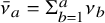
$\bar {\nu }_a = \Sigma _{b=1}^a \nu _b$
 . We refer to m as the length of
$\nu $
 .
We say that
$\nu $
 is a
$\sigma $
 -admissible shape if
$s_{i,j} = 0$
 for all
$\bar {\nu }_a + 1 \le i, j < \bar {\nu }_{a+1}$
 and
$a=1,...,m-1$
 . In [Reference Brundan and KleshchevBK06] these were simply referred to as admissible shapes. We note that
$(1^n)$
 is
$\sigma $
 -admissible for every
$\sigma $
 , and that for each
$\sigma $
 there is a unique
$\sigma $
 -admissible shape of minimal length, which is known as the minimal admissible shape.
From a
$\sigma $
 -admissible shape we can construct a relative shift matrix
$\sigma (\nu )$
 , which is an
$m \times m$
 -matrix with entries
$s(\nu )_{i,j}$
 in
$\mathbb {Z}_{\ge 0}$
 determined by

Since
$s_{i, i+1} = 0$
 for all
$i = \bar {\nu }_a, \bar {\nu }_a+1,...,\bar {\nu }_{a+1}-1$
 , and
$\sigma $
 can be recovered from its super-diagonal entries, it follows that
$\sigma $
 can be recovered from the pair
$(\sigma (\nu ), \nu )$
 .
Similarly, if we fix a level
$\ell $
 and let
$\lambda = (\lambda _1,...,\lambda _n)$
 be the partition determined by the data
$(\sigma , \ell )$
 then we can define the relative partition
$\lambda (\nu ) = (\lambda (\nu )_1,...,\lambda (\nu )_m)$
 by
$\lambda (\nu )_a = \lambda _{\bar {\nu }_a}$
 . As above, we may recover
$\lambda $
 from the pair
$(\lambda (\nu ), \nu )$
 .
Now fix
$\beta = \pm 1$
 . We say that a
$\sigma $
 -admissible shape
$\nu $
 is
$(\beta , \sigma )$
 -admissible if
$\beta ^{\nu _a} = 1 $
 for
$a=1,...,m$
 . When
$\beta =-1$
 this ensures that
$\nu _a$
 are all even, whilst for
$\beta =1$
 any
$\sigma $
 -admissible shape is
$(\beta , \sigma )$
 -admissible.
The notation of a
$(\beta , \sigma )$
 -admissible shape is key to our later constructions and so we would like to motivate it here. In Theorem 5.3 we introduce an involution on the shifted current Lie algebra
$\mathfrak {c}_n(\sigma )$
 , and the involution extends to the current algebra
$\mathfrak {c}_n$
 . On the zero graded piece
$\mathfrak {gl}_n \subseteq \mathfrak {c}_n$
 , the matrix of the involution is symmetric when
$\beta = 1$
 and antisymmetric when
$\beta = -1$
 . This is a shadow of the fact, central to our work: the (semiclassical) shifted twisted Yangian of type AI surjects onto classical finite W-algebras for which there are no multiplicity constraints on the partition of the nilpotent element, whilst the (as-yet-undefined) shifted twisted Yangian of type AII surjects onto those algebras for which there are multiplicity constraints (cf. Section 2.4). In this paper the role of the shifted twisted Yangian of type AII is played by the Dirac reductions with
$\beta = -1$
 appearing in Theorem C.
2.3 Classical finite W-algebras
Let
$\mathfrak {g}$
 be the Lie algebra of a connected complex reductive group G. A nilpotent orbit of
$\mathbb {O} \subseteq \mathfrak {g}$
 is a G-orbit consisting of elements which act nilpotently on every finite dimension representation. Let
$\kappa $
 be a choice of G-invariant nondegenerate bilinear form on
$\mathfrak {g}$
 .
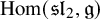
The Jacobson–Morozov theorem states that nilpotent G-orbits are in 1-1 correspondence with the G-orbits in the space of Lie algebra homomorphisms
$\operatorname {Hom}(\mathfrak {sl}_2, \mathfrak {g})$
 . The bijection is provided by choosing a nonzero nilpotent element
$e\in \mathfrak {sl}_2$
 and sending
$\phi \in \operatorname {Hom}(\mathfrak {sl}_2, \mathfrak {g})$
 to
$G\cdot \phi (e)$
 . Inverting this map we may associate an
$\mathfrak {sl}_2$
 -triple
$(e,h,f)$
 to any nilpotent element
$e\in \mathfrak {g}$
 , unique up to conjugacy.
The grading
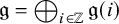
$\mathfrak {g} = \bigoplus _{i\in \mathbb {Z}} \mathfrak {g}(i)$
 induced by
$\operatorname {ad}(h)$
 is called the Dynkin grading, and the variety
$e + \mathfrak {g}^f \subseteq \mathfrak {g}$
 is called the Slodowy slice to
$\mathbb {O}$
 . By
$\mathfrak {sl}_2$
 -theory
$T_e \mathbb {O} = \operatorname {ad}(\mathfrak {g})e$
 and
$T_e(e+ \mathfrak {g}^f) = \mathfrak {g}^f$
 are mutually orthogonal complements inside
$\mathfrak {g}$
 with respect to the Killing form, and so the slice is transversal to the orbit of e (in fact, to every orbit which it intersects).
Let
$G(<0)$
 be the unipotent subgroup of G with Lie algebra
$\mathfrak {g}(<0) = \bigoplus _{i<0} \mathfrak {g}(i)$
 . Thanks to [Reference Gan and GinzburgGG02, Lemma 2.1] we have an isomorphism

of
$G(<0)$
 -varieties, where
$G(<0)$
 acts by left multiplication on the left hand factor, and via the adjoint action on the right hand side. We define the classical finite W-algebra to be the subquotient

where
$\mathfrak {g}(\le 0)_e := \{x - \kappa (e,x) \mid x\in \mathfrak {g}(\le 0)\}$
 . Using (2.5) we identify
$S(\mathfrak {g},e)$
 with
$\mathbb {C}[e + \mathfrak {g}^f\!]$
 as commutative algebras.
We can equip
$S(\mathfrak {g},e)$
 with a Poisson structure, using a version of Hamiltonian reduction (see [Reference Ambrosio, Carnovale, Esposito and TopleyACET20, §3.1], for example). Describing this Poisson structure is the main goal of the present article.
2.4 Nilpotent orbits in classical Lie algebras
Pick
$\varepsilon = \pm 1$
 and an integer
$N> 0$
 satisfying
$\varepsilon ^N = 1$
 . Suppose that
$(\cdot , \cdot ) : \mathbb {C}^N \times \mathbb {C}^N \to \mathbb {C}$
 is a form satisfying
$(u,v) = \varepsilon (v,u)$
 for all
$u,v\in \mathbb {C}^N$
 . The Lie algebra subalgebra
$\mathfrak {g}_0$
 of
$\mathfrak {gl}_N$
 consisting of skew-self adjoint matrices with respect to
$(\cdot , \cdot )$
 is a classical simple Lie algebra. More precisely
$\mathfrak {g}_0 \cong \mathfrak {sp}_N$
 when
$\varepsilon = -1$
 and
$\mathfrak {g}_0 \cong \mathfrak {so}_N$
 when
$\varepsilon = 1$
 . The connected component of the subgroup of
$\operatorname {GL}_N$
 preserving the form
$(\cdot , \cdot )$
 is denoted
$G_0$
 .
The nilpotent
$\operatorname {GL}_N$
 -orbits in
$\mathfrak {gl}_N$
 are parameterised by partitions
$\lambda \vdash N$
 , thanks to the theory of Jordan normal form. If
$\mathbb {O}_\lambda $
 is the orbit corresponding to
$\lambda \vdash N$
 then
$\mathbb {O}_\lambda \cap \mathfrak {g}_0$
 is either empty or is a union of at most two
$G_0$
 -orbits [Reference Collingwood and McGovernCM93, §5]. In particular,
$\mathbb {O}_\lambda \cap \mathfrak {g}_0 \ne \emptyset $
 if and only if:
-
• $(\varepsilon = 1)$
all even parts of
$\lambda $
occur with even multiplicity, -
• $(\varepsilon = -1)$
all odd parts of
$\lambda $
occur with even multiplicity.


We denote the set of partitions satisfying these conditions by
$\mathcal {P}_\varepsilon (N)$
 . A partition
$\lambda \in \mathcal {P}_\varepsilon (N)$
 is called even if all parts of
$\lambda $
 have the same parity.
Also, for
$\lambda \in \mathcal {P}_\varepsilon (N)$
 we note that
$\mathbb {O}_\lambda \cap \mathfrak {g}_0$
 is a union of two
$G_0$
 -orbits if and only if
$\varepsilon = 1$
 and all parts of
$\lambda $
 are even; such partitions are called very even. In all other cases,
$\mathbb {O}_\lambda \cap \mathfrak {g}_0$
 is a single orbit.
2.5 Dirac reduction for fixed points
Let A be an affine Poisson algebra with a group H of Poisson automorphisms. The ideal of coinvariants is denoted
$I_H = (h \cdot a - a\mid h\in H, \ a\in A)$
 . The H-fixed points
$I_H^H \subseteq I_H$
 are a Poisson ideal of
$A^H$
 and the Dirac reduction of A by H is the Poisson algebra

It is explained in [Reference TopleyTo23, §2.1] that when
$X = \operatorname {Spec}(A)$
 is an affine Poisson variety the Dirac reduction equips
$X^H$
 with the structure of an affine Poisson scheme, see also [Reference Laurent-Gengoux, Pichereau and VanhaeckeLPV13, §5.4.3].
Now retain the notation of Section 2.3. We suppose that
$H \subseteq \operatorname {Aut}(\mathfrak {g})$
 is a reductive group of automorphisms fixing the
$\mathfrak {sl}_2$
 -triple pointwise. Then H induces a group of Poisson automorphisms of
$S(\mathfrak {g},e)$
 . We write
$\mathfrak {g}_0 = \mathfrak {g}^H$
 for the fixed point subalgebra, which is also the Lie algebra of a reductive group [Reference TopleyTo23, Lemma 2.5(2)]. One of the main applications of Dirac reduction, in the context of the present work, is the following.
Theorem 2.2 [Reference TopleyTo23, Theorem 2.6].
There is an isomorphism of Poisson algebras

3 Shifted twisted Yangian versus Dirac reduction of shifted Yangians
3.1 Twisted Yangian
We refer the reader to [Reference MolevMo07, Ch. 2] for a good introduction to Olshanski’s theory of twisted Yangians.
Recall that the twisted Yangian
$\mathcal {Y}_n$
 associated to
$\mathfrak {o}_n$
 is generated by elements
$\{ s_{i,j}^{(r)} \mid 1\le i,j \le n, r \ge 0\} $
 subject to the quaternary and symmetry relation [Reference MolevMo07, Proposition 2.2.1]. In [Reference Lu, Wang and ZhangLWZ23] those authors solved the long-standing problem of providing a Drinfeld presentation of
$\mathcal {Y}_n$
 associated to the split bilinear form on
$\mathbb {C}^n$
 . These are known as twisted Yangians of type AI, and from now on we will focus on type AI.
We recall the main results of their their paper, which is the Drinfeld presentation of
$\mathcal {Y}_n$
 , see [Reference Lu, Wang and ZhangLWZ23, Theorem 5.1].
Theorem 3.1. Let
$C=(c_{ij})_{1\le i,j\le n-1}$
 be the Cartan matrix of type
$\mathsf {A}_{n-1}$
 , and set
$h_{i,-1}=1$
 ,
$c_{0j}=-\delta _{j,1}$
 . Then the twisted Yangian
$\mathcal {Y}_n$
 is generated by

subject only to the following relations, for
$r,s \in \mathbb {N}$
 :


where
$\mathrm {Sym}_{k_1, k_2}$
 denotes the sum of the two expressions obtained by permuting
$k_1, k_2$
 and
$[ a, b]_- := ab + ba$
 denotes the anticommutator.
We equip
$\mathcal {Y}_n$
 with the loop filtration, by placing
$h_{i,r}$
 and
$b_{i,r}$
 in degree r. We also equip
$\mathcal {Y}_n$
 with the canonical filtration by placing
$h_{i,r}$
 and
$b_{i,r}$
 in degree
$r + 1$
 and the Poisson bracket in degree
$-1$
 . We will denote the corresponding associated graded algebras by
$\operatorname {gr}_L \mathcal {Y}_{n}$
 and
$\operatorname {gr}_C \mathcal {Y}_{n}$
 for the loop and canonical filtrations, respectively.
Analogously to [Reference Lu, Wang and ZhangLWZ23, Proof of Theorem 5.1] we inductively define elements

and let
$b_{i,j}^{(r)}:=(-1)^{(r-1)}b_{j,i}^{(r)}$
 for
$i < j$
 .
3.2 Shifted twisted Yangian and the semiclassical limit
Retain the notation of Theorem 3.1. Let
$\sigma = (s_{i,j})_{1\le i, j \le N}$
 be a symmetric
$n \times n$
 shift matrix. We define the shifted twisted Yangian
$\mathcal {Y}_n(\sigma )$
 to be the associative algebra generated by the elements

subject to relations (3.2)–(3.6) for all admissible indexes (i.e., whenever the indexes make sense). This algebra is equipped with a loop filtration, again placing
$h_{i,r}$
 and
$b_{i,r}$
 in degree r, and a canonical filtration which places those same elements in degree
$r+1$
 . We will denote the corresponding associated graded algebras by
$\operatorname {gr}_L \mathcal {Y}_{n}(\sigma )$
 for the loop filtration and by
$\operatorname {gr}_C \mathcal {Y}_{n}(\sigma )$
 for the canonical filtration respectively. Similar to (3.7) we define elements

and let
${}^{\sigma }b_{i,j}^{(r)}:=(-1)^{(r-1)}{}^{\sigma }b_{j,i}^{(r)}$
 for
$i < j$
 .
Theorem 3.2.
-
(1) The map $\mathcal {Y}_n(\sigma ) \to \mathcal {Y}_n$
sending (3.10) $$ \begin{align} \begin{array}{rcl} b_{i, r} & \longmapsto & b_{i,r}\\h_{i,r} & \longmapsto & h_{i,r}. \end{array} \end{align} $$is an injective filtered homomorphism with respect to both the loop filtration and the canonical filtration.
-
(2) $\mathcal {Y}_n(\sigma )$
has a PBW basis consisting of ordered monomials in the elements $$ \begin{align*}\{ h_{i,r}, {}^\sigma b_{j,k}^{(s)} \mid 0 \le i < n, \ \ 1\le k < j \le n,\ \ r \ge 0, \ \ s \ge s_{j, k} \}.\end{align*} $$



Proof. It is clear that the map is a filtered homomorphism with respect to both filtrations. As the map
$\mathcal {Y}_N(\sigma ) \to \mathcal {Y}_N$
 is filtered with respect to the loop filtration it induces a map
$\operatorname {gr}_L \mathcal {Y}_N(\sigma ) \to \operatorname {gr}_L \mathcal {Y}_N$
 . We will write
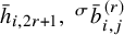
$\bar {h}_{i,2r+1}, \ {}^{\sigma }\bar {b}_{i,j}^{(r)}$
 for the images of
$h_{i,2r+1}, \ {}^{\sigma }b_{i,j}^{(r)}$
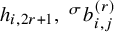 in
$\operatorname {gr}_L \mathcal {Y}_N(\sigma )$
 . It then follows from [Reference Lu, Wang and ZhangLWZ23, (5.3)] that the map on the associated graded sends
${}^{\sigma }\bar {b}_{i,j}^{(r)} \in \operatorname {gr}_L \mathcal {Y}_N(\sigma )$
 to
$\bar {b}_{i,j}^{(r)} \in \operatorname {gr}_L \mathcal {Y}_N$
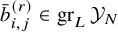 as defined in [Reference Lu, Wang and ZhangLWZ23, §5.4] but from the proof of [Reference Lu, Wang and ZhangLWZ23, Theorem 5.1] we see that the ordered monomials in the elements
$\bar {h}_{i,2r+1}, \ \bar {b}_{i,j}^{(r)}$
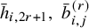 are linearly independent in
$\operatorname {gr}_L \mathcal {Y}_n$
 . In particular the ordered monomials in the elements
$h_{i,2r+1}, {}^{\sigma }b_{i,j}^{(r)} \in \mathcal {Y}_N(\sigma ) $
 are linearly independent too.
Following the proof of [Reference Lu, Wang and ZhangLWZ23, Theorem 5.1] verbatim it is easy to see that the ordered monomials in the elements
$h_{i,2r+1}, {}^{\sigma }b_{j,k}^{(s)}$
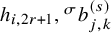 for
$0 \leq i < n, \ 1 \leq k<j < n, \ r \in \mathbb {N}, \ s \geq s_{j,k}$
 span
$\mathcal {Y}_n(\sigma )$
 . Hence the map is injective.
We recall the definition of the shifted current algebra
$\mathfrak {c}_n(\sigma ) \subseteq \mathfrak {gl}_n[z] = \mathfrak {gl}_n \otimes \mathbb {C}[z]$
 from [Reference TopleyTo23, (3.3)]. First define the current algebra
$\mathfrak {c}_n$
 to be
$\mathfrak {gl}_n[z]$
 with Lie bracket given by
$[a\otimes f), b\otimes g] = [a,b] \otimes fg$
 , where
$a, \in \mathfrak {gl}_n$
 and
$f,g \in \mathbb {C}[t]$
 . Then
$\mathfrak {c}_n(\sigma )$
 is the Lie subalgebra of
$\mathfrak {c}_n$
 spanned by the elements
$e_{i,j}z^r$
 for
$1\le i,j \le n$
 and
$r \ge s_{i,j}$
 .
Let
$\tau :\mathfrak {gl}_n \to \mathfrak {gl}_n: A \mapsto -A^T$
 . We define the twisted shifted current algebra for
$\mathfrak {so}_n$
 to be
$\mathfrak {c}_n(\sigma )^{\tau }:=\{A(z) \in \mathfrak {c}_n(\sigma ) \mid A(z)= \tau (A(-z)) \}$
 .
Lemma 3.3.
-
(1) We have a natural isomorphism $U(\mathfrak {c}_n(\sigma )^{\tau }) \to \operatorname {gr}_L \mathcal {Y}_n(\sigma )$
given by (3.11) $$ \begin{align} e_{i,j}z^r+(-1)^{r-1}e_{j,i}z^r \mapsto {}^{\sigma}b_{i,j}^{(r)}+F^{L}_{r-1}\mathcal{Y}_n \end{align} $$
-
(2) We have a natural isomorphism of commutative algebras $S(\mathfrak {c}_n(\sigma )^{\tau }) \to \operatorname {gr}_C \mathcal {Y}_n(\sigma )$
given by (3.12) $$ \begin{align} e_{i,j}z^r+(-1)^{r-1}e_{j,i}z^r \mapsto {}^{\sigma}b_{i,j}^{(r)}+F^{C}_{r}\mathcal{Y}_n \end{align} $$




Proof. We let
${}^{\sigma }\bar {b}_{i,j}^{(r)}$
 denote
${}^{\sigma }{b}_{i,j}^{(r)}+F^{L}_{r-1}\mathcal {Y}_n(\sigma )$
 . Following the proof of [Reference Lu, Wang and ZhangLWZ23, (5.11)] verbatim we obtain the relation

and hence the map in (1) is a homomorphism of algebras. It is easy to see that
$\mathfrak {c}_n(\sigma )^{\tau }$
 has a basis consisting of
$e_{i,j}z^r+(-1)^{r-1}e_{j,i}z^r, \ i>j, \ r \geq s_{i,j}$
 together with
$e_{i,i}z^{2r+1}$
 and hence the ordered monomials in these elements form a basis for
$U(\mathfrak {c}_n(\sigma )^{\tau })$
 . By Theorem 3.2 the ordered monomials in the elements
${}^{\sigma }b_{i,j}^{(r)}, \ i>j, \ r \geq s_{i,j}$
 together with
$b_{i,i}^{(2r+1)}$
 form a basis for
$\mathcal {Y}_n(\sigma )$
 and hence our map is an isomorphism. For part (2) using the definition of the twisted Yangian as in [Reference Lu, Wang and ZhangLWZ23, Definition 2.1] we define a filtration by putting the generators
$s_{i,j}^{(r)}$
 in degree r. By [Reference MolevMo07, Theorem 2.4.3] we see that the associated graded algebra is commutative with bracket in degree
$-1$
 . Using [Reference Lu, Wang and ZhangLWZ23, (3.1), (3.12)-(3.13)] it follows that this filtration lines up with the canonical filtration on
$\mathcal {Y}_n$
 and hence
$\operatorname {gr}_C \mathcal {Y}_n$
 is commutative. The map defined in Theorem 3.2 is a filtered injection and hence also
$\operatorname {gr}_C \mathcal {Y}_n(\sigma )$
 is commutative. The current theorem then follows by part (1).
Before we proceed we take a brief digression to discuss presentations of Poisson algebras. The free Poisson algebra generated by a set X is the symmetric algebra
$S(L_X)$
 of the free Lie algebra
$L_X$
 generated by the set X. A Poisson presentation of a Poisson algebra A is an exact sequence of the form

where
$I \subseteq S(L_X)$
 is a Poisson ideal. The generators of the Poisson ideal will be referred to as Poisson relations. In the sequel it will be important to distinguish between generators of A viewed as a commutative algebra and as a Poisson algebra, and so we emphasise this terminology whenever any ambiguity is possible. We refer the reader to [Reference TopleyTo23, §3.1] for slightly more detail.
Proposition 3.4. Let
$A=(c_{ij})_{1\leq i,j\leq n-1}$
 be the Cartan matrix of type
$\mathsf {A}_{n-1}$
 , and set
$h_{i,-1}=1$
 ,
$c_{0j}=-\delta _{j,1}$
 . Then
$\operatorname {gr}_C \mathcal {Y}_n(\sigma )$
 is Poisson generated by
$h_{i,r}$
 ,
$ b_{j,s}$
 , for
$0\leq i<n$
 ,
$1\leq j<n$
 and
$r\in \mathbb {N}, s \geq s_{i+1,i}$
 subject only to the following relations:


Proof. Let
$\widehat {y}_n(\sigma )$
 be the algebra with generators and relations as in the statement of the Proposition. From relations (3.2)–(3.6) it follows that there is a canonical surjection
$\widehat {y}_n(\sigma )$
 . We inductively define elements in
$\widehat {y}_n(\sigma )$


and let
${}^{\sigma }b_{i,j}^{(r)}:=(-1)^{(r-1)}{}^{\sigma }b_{j,i}^{(r)}$
 for
$i < j$
 . We also define a loop filtration on
$\widehat {y}_n(\sigma )$
 by putting the generators in degree r and denote the counterparts of the
$^\sigma b_{i,j}^{(r)}$
 in
$\operatorname {gr}_L\widehat {y}_n(\sigma )$
 by
$^\sigma \bar {b}_{i,j}^{(r)}$
 . Once more following the proof of [Reference Lu, Wang and ZhangLWZ23, (5.11)] verbatim we get

so that
$\widehat {y}_n(\sigma )$
 is spanned by monomials in the elements
$h_{i,2r+1},{}^{\sigma }b_{i,j}^{(r)} \in \widehat {y}_n(\sigma )$
 . By Lemma 3.3
$\operatorname {gr}_C \mathcal {Y}_{n}(\sigma )$
 is a polynomial ring in the images of these maps under the canonical surjection so that the canonical surjection is an isomorphism.
3.3 The Dirac reduction of a shifted twisted Yangian
We continue to fix
$n> 0$
 , choose an
$n\,{\times}\, n$
 symmetric shift matrix
$\sigma $
 and fix
$\varepsilon \in \{\pm 1\}$
 . The (semiclassical) shifted Yangian
$y_n(\sigma )$
 is the Poisson algebra with Poisson generators

and Poisson relations [Reference TopleyTo23, (3.37)-(3.48)]. Following [Reference TopleyTo23, (3.58)] we introduce an involution on
$y_n(\sigma )$


Theorem 3.5. Let
$\sigma $
 be a symmetric shift matrix, let
$y_n(\sigma )$
 denote the corresponding semiclassical shifted Yangian and let
$\tau $
 denote the automorphism of
$y_n(\sigma )$
 introduced in (3.22). The Dirac reduction
$R(y_n(\sigma ), \tau )$
 is Poisson generated by elements

together with the following relations


where we adopt the convention
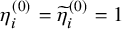
$\eta _i^{(0)} = \widetilde {\eta }_i^{(0)} = 1$
 and the elements
$\widetilde {\eta }_i^{(2r)} $
 are defined via the recursion

Furthermore we define

Proof. (3.24)-(3.29) are as in [Reference TopleyTo23, Theorem 3.7]. We claim that (3.30) is equivalent to [Reference TopleyTo23, (3.74)] which says

Making the substitution
$q:=m-m_1-1$
 in the first sum this now reads as

now changing the order of summation in the first sum this reads as

which is as claimed.
Remark 3.6. Relation (3.26) is actually different from [Reference TopleyTo23, (3.70)] and we have replaced
$\varpi _{r,s}$
 with
$\varpi _{s,r}$
 . This is due to the fact that [Reference TopleyTo23, (3.70)] actually should read as our relation (3.26) as is evident from the proof of [Reference TopleyTo23, Thm. 3.7] but a sign mistake appears in the relation [Reference TopleyTo23, (3.70)] which is fixed by replacing
$\varpi _{r,s}$
 with
$\varpi _{s,r}$
 .
3.4 Proof of Theorem A
We now introduce certain elements in
$R(y_n(\sigma ),\tau )$
 whose role will become clear later on. Let


Remark 3.7. Define the following formal power series


Note that for
$i>1$
 the
$\bar {\eta }^{(2r)}_i$
 are the coefficients of
$t^{-2r}$
 of the power series
$ \bar {\eta }_i(u):=\tilde {\eta }_{i-1}(u) \eta _{i}(u)$
 . By the recursion (3.31) we see that
$ \tilde {\eta }_{i}(u) \eta _{i}(u)=1$
 . In particular this gives
$\eta _{i}(u)= \bar {\eta }_{1}(u) \dots \bar {\eta }_{i}(u) $
 so that we can recover monomials in the elements
$\eta _{i}^{(2r)}, 1 \leq i \leq n, \ r \geq 0$
 from monomials in the elements
$\bar {\eta }_{i}^{(2r)}, 1 \leq i \leq n, \ r \geq 0$
 and vice versa. In particular, the elements

are a set of Poisson generators of
$R(y_n(\sigma ), \tau )$
 , thanks to Theorem 3.5.
The following Lemma will prove useful later on.
Lemma 3.8. The following equalities hold in
$R(y_n(\sigma ),\tau )$



Proof. The first one of these relations follows immediately by relation (3.24) as
$\bar {\eta }^{(2r)}_i$
 is polynomial in
$\eta _i^{2r},\eta _{i-1}^{2s}, \ 1 \leq r,s$
 . The second relation is proved just as [Reference TopleyTo23, (3.56)]. For the third relation we have

where the second equality follows by (3.25) and (3.39). Thus the coefficient of
$\theta _j^{(s+1+2k)}, \ 0 \leq k \leq r-1$
 is given by
$((\delta _{i-1,j+1}-\delta _{i-1,j})+(\delta _{i,j}-\delta _{i,j+1}))\sum _{w=0}^{r-j-1}\eta _{i}^{(w)}\tilde {\eta }_{i-1}^{(2r-2w-2j-2)}$
 which proves the lemma.
Theorem 3.9. The semiclassical limit of the shifted twisted Yangian
$y_n^{+}(\sigma ):=\operatorname {gr}_C \mathcal {Y}_n(\sigma )$
 is isomorphic, as a Poisson algebra, to the Dirac reduction
$R(y_n(\sigma ), \tau )$
 , with respect to the involution (3.22).
Proof. Consider the map
$ \operatorname {gr}_C \mathcal {Y}_n(\sigma ) \to R(y_n(\sigma ),\tau ) $
 given by

Using relations (3.25)-(3.30) together with (3.38) and (3.40) it is readily verified that the map is a morphism of Poisson algebras. Indeed to check (3.14) use (3.38), to check (3.15) use (3.40), to check (3.16) use (3.26) and (3.27), to check (3.17) use (3.28) and to check (3.18) use (3.29),(3.30) and (3.40). By the proof of [Reference TopleyTo23, Theorem 3.7] we know that
$R(y_n(\sigma ))$
 has a basis consisting of monomials in
$\eta _{i}^{(2r)},\theta _{i,j}^{(s)}, 1 \leq i < j \leq n, r \geq 0, s> s_{i,j}$
 where the
$\theta _{i,j}^{(s)}$
 are defined inductively via the recursion

By definition of the map we see that
${}^{\sigma }b_{j,i}^{(r-1)}$
 as defined in (3.9) maps to a nonzero scalar multiple of
$\theta _{i,j}^{(r)}$
 .
By Remark 3.7 it follows that the set of monomials in
$\bar {\eta }_{i}^{(2r)},\theta _{i,j}^{(s)}, 1 \leq i < j \leq n, r \geq 0, s> s_{i,j}$
 is a basis for
$R(y_n(\sigma ),\tau )$
 and thus our map sends a spanning set to a basis. Hence it is an isomorphism.
4 Finite W-algebras for classical Lie algebras
4.1 Centralisers in general linear Lie algebras
Fix
$N> 0$
 and let
$\lambda $
 be a partition of N. Following Lemma 2.1 we let
$\sigma $
 be the shift matrix associated to
$\lambda $
 . Let
$\nu $
 be a
$\sigma $
 -admissible shape, and resume the notation
$\sigma (\nu )$
 and
$\lambda (\nu )$
 for the relative shift matrix and relative partition, defined in Section 2.2.
We introduce symbols
$\{u_{a,i,j} \mid 1\le a \le m, \ 1\le i \le \nu _m, \ 1\le j \le \lambda (\nu )_a\}$
 and identify
$\mathbb {C}^N$
 with the vector space with basis
$u_{a,i,j}$
 . The general linear Lie algebra
$\mathfrak {g} := \mathfrak {gl}_N$
 has a basis

where
$e_{a,i,j;b,k,l} u_{c,r,s} = \delta _{b,c}\delta _{k,r} \delta _{l, s} u_{a,i,j}$
 , so that

We pick the nilpotent element in
$\mathfrak {g}$
 by the rule

It has Jordan blocks of sizes
$\lambda _1,...,\lambda _{n}$
 . We also define a semisimple element
$h\in \mathfrak {gl}_N$
 by

The pair
$\{e,h\}$
 can be completed to an
$\mathfrak {sl}_2$
 triple
$\{e,h,f\} \subseteq \mathfrak {g}$
 . The Dynkin grading
$\mathfrak {g} = \bigoplus _{i\in \mathbb {Z}} \mathfrak {g}(i)$
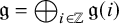 given by eigenspaces of
$\operatorname {ad}(h)$
 is a good grading, in the sense of [Reference Elashvili and KacEK05]. It is determined by

and so, in particular,
$e \in \mathfrak {g}(2)$
 . For
$1\le a, b\le m$
 ,
$1\le i\le \nu _a$
 ,
$1\le k\le \nu _b$
 and
$r = s_{a,b}(\nu ), s_{a,b}(\nu )+ 1,..., s_{a,b}(\nu ) + \min (\lambda (\nu )_a, \lambda (\nu )_b) - 1$
 , we define elements

The following description of the centraliser is given in [Reference TopleyTo23, Lemma 4.1], see [Reference YakimovaYa10, §1] for more detail. In [Reference TopleyTo23] two indices were used to describe a basis for
$\mathbb {C}^N$
 , whilst here we use three indices. Translating between these two conventions is an easy exercise.
Lemma 4.1. The centraliser
$\mathfrak {g}^e$
 has a basis consisting of elements

and the Lie bracket is given by

Furthermore
$\mathfrak {g}^e$
 is a Dynkin graded subalgebra of
$\mathfrak {g}$
 with
$c_{a,i,b,k}^{(r)}$
 lying in degree
$2r$
 .
4.2 Symplectic and orthogonal subalgebras
Fix
$N> 0$
 an integer and
$\varepsilon = \pm 1$
 such that
$\varepsilon ^N = 1$
 . We keep the partition
$\lambda $
 and shift matrix
$\sigma $
 from Section 4.1, let
$\beta = -\varepsilon (-1)^{\lambda _1}$
 , and we now also assume that
$\lambda \in \mathcal {P}_\varepsilon (N)$
 and that
$\nu $
 is
$(\beta , \sigma )$
 -admissible.
Consider the matrix

This is a block diagonal matrix can be described as follows. For each index
$a = 1,...,m$
 there is a block of size
$\nu _{a}\lambda (\nu )_a$
 , and each of these blocks is an antidiagonal matrix with entries
$\pm 1$
 . Furthermore, when
$\varepsilon = 1$
 the matrix J is symmetric and when
$\varepsilon = -1$
 it is antisymmetric.
Now define an involution of
$\mathfrak {g} = \mathfrak {gl}_N$
 by the rule

We decompose
$\mathfrak {g} = \mathfrak {g}_0 \oplus \mathfrak {g}_1$
 into eigenspaces for
$\tau $
 so that
$\mathfrak {g}_0$
 is the space of
$\tau $
 -invariants. Note that J is symmetric and
$\mathfrak {g}_0 \cong \mathfrak {so}_N$
 for
$\varepsilon =1$
 , whilst J is antisymmetric and
$\mathfrak {g}_0 \cong \mathfrak {sp}_N$
 for
$\varepsilon = -1$
 .
By Lemma 4.2(ii) we have
$\{e,h\}\subseteq \mathfrak {g}_0$
 , whilst
$f\in \mathfrak {g}_0$
 thanks to [Reference Collingwood and McGovernCM93, Lemma 3.4.4]. Write
$G_0$
 for the connected component of the subgroup of
$\operatorname {GL}_N$
 consisting of elements which preserve the bilinear form associated to J, so that
$G_0$
 is connected and
$\operatorname {Lie}(G_0) = \mathfrak {g}_0$
 .
Lemma 4.2. For all admissible indices we have:
-
(i) $\tau (e_{a,i,j;b,k,l}) = (\beta )^{i+k}(-1)^{j +l + 1} e_{b,\nu _b + 1 - k, \lambda (\nu )_b + 1 - l; a,\nu _a + 1 - i, \lambda (\nu )_a + 1 - j}$
; -
(ii) $\tau (e) = e$
and
$\tau (h)=h$
; -
(iii) $\tau (c_{a,i,b,k}^{(r)}) = (\beta )^{i+k}(-1)^{r-\frac {\lambda _k - \lambda _i}{2} - 1}c_{b,\nu _b + 1 - k,a, \nu _a + 1 - i}^{(r)}.$




Proof. Part (i) is proven using the fact that
$J^{-1} = \epsilon J$
 , and multiplying matrices, bearing in mind the fact that the
$\lambda _i$
 all have the same parity. Now (ii) and (iii) follow by applying (i) to (4.3), (4.4) and (4.6).
Remark 4.3. Henceforth the symbolic complexity will get somewhat more complicated, and to ease notation we introduce a certain involution on our index sets. Whenever we have a four-tuple of indices
$(a,i,b,k)$
 in the ranges
$1 \le a,b \le m, \ 1 \le i \le \nu _a, \ 1 \le k \le \nu _b$
 we will write

Similarly for a six-tuple
$(a,i,j;b,k,l)$
 with indexes in the range
$1\le a,b \le m, 1\le i\le \nu _a, 1\le k \le \nu _b, 1\le j\le \lambda (\nu )_a, 1\le l \le \lambda (\nu )_b)$
 so that, for example, Lemma 4.2 (i) could be read as

4.3 Generators of the classical finite W-algebra
Here we reproduce formulas for the Poisson generators of
$S(\mathfrak {gl}_N, e)$
 discovered by Brundan and Kleshchev in their seminal work [Reference Brundan and KleshchevBK06, §9], in which they gave presentations of the noncommutative finite W-algebras associated to
$\mathfrak {gl}_N$
 . The results of this section generalise [Reference TopleyTo23, §4.3] to the parabolic setting. Retain all of the choices and notation from Section 4.2.
Now for
$1 \le a,b \le m$
 ,
$1 \le i \le \nu _a$
 ,
$1 \le k \le \nu _b$
 ,
$0 \le x < n$
 and
$r> 0$
 , we let

where we use the symbol

and the second summation is taken over all
$6$
 -tuples of indices
$(a_u,i_u, j_u,b_u, k_u, l_u)_{u=1,...,s}$
 in the ranges

satisfying the following six conditions:
-
(a) $\sum _{u=1}^s (2l_u - 2j_u) + \lambda (\nu )_{a_u} - \lambda (\nu )_{b_u} = 2(r - s)$
; -
(b) $2l_u- 2j_u + \lambda (\nu )_{a_u} - \lambda (\nu )_{b_u} \ge 0$
for each
$u = 1,\dots ,s$
; -
(c) if $\bar {\nu }_{b_u-1}+k_u> x$
, then
$l_u < j_{u+1}$
for each
$u = 1,\dots ,s-1$
; -
(d) if $\bar {\nu }_{{b_u}-1}+k_u \le x$
then
$l_u \ge j_{u+1}$
for each
$u = 1,\dots ,s-1$
; -
(e) $a_1 = a$
,
$i_1 = i$
,
$b_s = b$
and
$k_s = k$
. -
(f) $b_u = a_{u+1}$
and
$k_u = i_{u+1}$
for all
$u=1,...,s-1$
.










Fixing
$r> 0$
 and choosing
$s \in \{1,...,r\}$
 we make the notation
$\mathcal {X}_{a,i,b,k; x}^{(r, s)}$
 for the set of ordered sets
$(a_u,i_u, j_u,b_u, k_u, l_u)_{u = 1}^s$
 in the range (4.14) satisfying the conditions (a)–(f) and consider the map

It is clear that this is an involution on collections of ordered sets in the range (4.14), and we now prove that it respects the conditions (a)-(f).
Lemma 4.4. For all
$t=1,...,s$
 the map
$\upsilon $
 defines a bijection

Proof. The index bounds (4.14) ensure that
$\mathcal {X}_{a,i,b,k, \bar {\nu }_t}^{(r,s)}$
 is finite. Since
$\upsilon ^2$
 is the identity map it will suffice to show that
$\upsilon $
 maps the left hand side of (4.15) to the right. We fix
$(a_u,i_u, j_u,b_u, k_u, l_u)_{u = 1,...,s}\in \mathcal {X}_{a,i,b,k; \bar {\nu }_t}^{(r,s)}$
 and check that conditions (a)–(f) hold for
$\upsilon (a_u,i_u, j_u, b_u, k_u, l_u)_{u=1,...,s}$
 . For example,

This shows that when (a) is satisfied for
$(a_u,i_u, j_u, b_u, k_u, l_u)_{u=1,...,s}$
 , it follows that the formulation of (a) which defines
$\mathcal {X}_{b, k' , a, i'; \bar {\nu }_t}^{(r,s)}$
 holds for
$\upsilon (a_u,i_u, j_u, b_u, k_u, l_u)_{u=1,...,s}$
 . Conditions (b)–(f) can be checked similarly.
Now we define a map
$\theta : \mathfrak {g}^e \to S(\mathfrak {g}(\operatorname {\ge \!0}))$
 by

for all admissible
$i,j,r$
 .
By (4.5) and Lemma 4.2(i) we see that
$\tau $
 induces an involution on
$\mathfrak {g}^e$
 and
$S(\mathfrak {g}(\operatorname {\ge \!0}))$
 , and the latter preserves
$S(\mathfrak {g},e)$
 .
Proposition 4.5.
$\theta : \mathfrak {g}^e \to S(\mathfrak {g},e)$
 is
$\tau $
 -equivariant.
Proof. The assertion that the image of
$\theta $
 lies in
$S(\mathfrak {g},e)$
 is an immediate consequence of [Reference Brundan and KleshchevBK06, Theorem 10.1], upon taking the top graded term with respect to the Kazhdan filtration of the finite W-algebra.
Thanks to Lemma 4.2(iii) the
$\tau $
 -equivariance will follow from (4.17). Fix indices
$1\le a, b \le m, 1 \le i \le \lambda (\nu )_a, 1 \le k \le \lambda (\nu )_b, \ 0\le x < n$
 and
$0 < r$
 . Choose
$s\in \{1,...,r\}$
 . Let
$(a_m,i_m, j_m, b_m, k_m,l_m)_{m=1}^s \in \mathcal {X}_{a,i,b,k; \bar {\nu }_t}^{(r,s)}$
 . Thanks to Lemma 4.2(i) we have

Conditions (a), (e), (f) imply that
$\sum _m (j_m - l_m + 1) = \frac {\lambda _{i_1} - \lambda _{k_s}}{2} - r.$
 Conditions (e), (f) imply
$(-1)^{\sum _{m=1}^s k_m+i_m}=(-1)^{i+k}$
 . Hence the sign on the right hand side of (4.17) is equal to
$(\beta )^{i+k}(-1)^{r-\frac {\lambda _k - \lambda _i}{2}}$
 . Furthermore condition (f) together with our condition on x ensures that
$\# \{ m =1,...,s-1 \mid \nu _1+\dots + \nu _{b_m-1}+k_m \le \bar {\nu }_t\} = \# \{m =2,...,s \mid \nu _1+\dots + \nu _{a_m-1}+\lambda (\nu )_m + 1 - i_m \le \bar {\nu }_t\}.$
 Combining these observations together with Lemma 4.4 we have

This completes the proof.
Lemma 4.6. For
$ s_{a,b} < r \le s_{a,b} + \min (\lambda (\nu )_a, \lambda (\nu )_b)$
 the linear parts of

respectively are

In particular
$\theta $
 fulfils the properties of [Reference TopleyTo23, Theorem 2.4].
Proof. The linear part of (4.12) corresponds to
$s=1$
 . Conditions (b)-(d) as well as condition (f) on the indices in (4.12) become redundant when
$s=1$
 whereas combining conditions (a) and (e) gives the sum

which is equal to
$(-1)^{r-1}c_{a,i,b,k}^{(r-1)}$
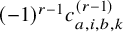 by definition 4.6.
5 Dirac reduction for shifted Yangians
5.1 Parabolic presentations for shifted current Lie–Poisson algebras
In this section we describe the parabolic Poisson presentations of shifted current Lie algebras. This is simultaneously a generalisation of [Reference TopleyTo23, §3.2], which implicitly treated the shape
$(1^n)$
 , and is a semiclassical analogue of the results of [Reference Brundan and KleshchevBK05].
We will repeatedly use the notion of a presentation of a Poisson algebra which was briefly explained before the statement of Proposition 3.4.
Throughout this section we fix
$n> 0$
 and a symmetric
$n\times n$
 shift matrix
$\sigma $
 . Pick an admissible shape
$\nu = (\nu _1,...,\nu _m)$
 for
$\sigma $
 , and recall the relative shift matrix
$\sigma (\nu )$
 , as well as the notation
$\bar {\nu }_a = \sum _{i=1}^a \nu _i$
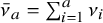 , introduced in Section 2.2.
The current algebra is the Lie algebra
$\mathfrak {c}_n := \mathfrak {gl}_n \otimes \mathbb {C}[t]$
 . We write
$e_{i,j}$
 for standard matrix units and
$e_{i,j}t^r := e_{i,j} \otimes t^r$
 . A basis is given by
$\{e_{i,j} t^r \mid 1\leq i , j \leq n, \ r \ge 0\}$
 .
We will need a parabolic labelling of the basis of
$\mathfrak {c}_n(\sigma )$
 . Define elements

We warn the reader that the notation used here for matrix units is different from that appearing in Section 4.1.
We define the shifted current algebra
$\mathfrak {c}_n(\sigma )$
 to be the subalgebra spanned by

Lemma 5.1. The Lie subalgebra
$^{\nu }\mathfrak {u}_n(\sigma ) \subseteq \mathfrak {c}_n(\sigma )$
 which is spanned by elements (5.2) with
$a< b$
 , has generators

and relations


Proof. Write
$\underline {0}$
 for the
$n\times n$
 zero matrix. It follows from (2.1) that the linear map
$^{\nu }\mathfrak {u}_n(\sigma ) \to ^{\nu }\mathfrak {u}_n(\underline {0})$
 defined by
$e_{a,i,b,j}t^r \mapsto e_{a,i,b,j}t^{r-s_{a,b}}$
 is a Lie algebra isomorphism and so it suffices to prove the current lemma when
$\sigma = \underline {0}$
 .
Let
$^{\nu }\widehat {\mathfrak {u}}_n$
 be the Lie algebra with generators (5.3) and relations (5.4)–(5.6), with
$\sigma = \underline {0}$
 . We inductively define elements
$e_{a,i,b,j;r} \in {}^{\nu }\widehat {\mathfrak {u}}_n$
 by setting
$e_{a,i,a+1,j;r} := e_{a,i,j;r}$
 and
$e_{a,i,b,j;r} := [e_{a,i,k,b-1; r}, e_{b-1,k,j; 0}]$
 for
$1\le a < b \le m$
 and all admissible
$i,j$
 . There is a homomorphism
$^{\nu }\widehat {\mathfrak {u}}_n \twoheadrightarrow {}^{\nu }\mathfrak {u}_n(\underline 0)$
 given by
$e_{a,i,j;r} \mapsto e_{a,i,a+1,j}t^r$
 and, in order to show that it is an isomorphism, we show that
$^{\nu }\widehat {\mathfrak {u}}_n$
 is spanned by the elements
$\{e_{a,i,b,j;r} \mid 1\le a<b\le m, \ 1 \le i \le \nu _a, \ 1\le j \le \nu _b, \ 0 \le r\}$
 .
Following (1)–(7) in the proof of [Reference Brundan and KleshchevBK05, Lemma 6.7] verbatim we have for all
$a,b,c,d,j,k,l,r,s$


Define an ascending filtration on
$\widehat {\mathfrak {u}}_n = \bigcup _{d> 0} \operatorname {F}_d \widehat {\mathfrak {u}}_n$
 satisfying
$\operatorname {F}_{d} \widehat {\mathfrak {u}}_n = \sum _{\substack {d_1 + d_2 = d}} [\operatorname {F}_{d_1} \widehat {\mathfrak {u}}_n, \operatorname {F}_{d_2} \widehat {\mathfrak {u}}_n]$
 by placing
$e_{a,i,j;r}$
 in degree 1. We prove by induction that
$\operatorname {F}_d\widehat {\mathfrak {u}}_n$
 is spanned by elements
$e_{a,i,b,j;r}$
 with
$j-i \le d$
 . The base case
$d = 1$
 holds by definition. For
$d_1 + d_2 = d> 1$
 we know by the inductive hypothesis that
$\operatorname {F}_{d_1} \widehat {\mathfrak {u}}_n$
 and
$\operatorname {F}_{d_2} \widehat {\mathfrak {u}}_n$
 are spanned by elements
$e_{a,i,b,j;r}$
 . Using (5.7) we complete the induction, which finishes the proof.
Since
$\mathfrak {c}_n(\sigma )$
 is a Lie algebra the symmetric algebra
$S(\mathfrak {c}_n(\sigma ))$
 carries a natural Poisson structure.
Theorem 5.2. Let
$\sigma $
 be a symmetric shift matrix
$\nu =(\nu _1,\dots ,\nu _m)$
 an admissible shape and let
$\mathfrak {c}_n(\sigma )$
 denote the shifted current algebra. Then
$S(\mathfrak {c}_n(\sigma ))$
 is Poisson generated by

subject to relations


Proof. By [Reference TopleyTo23, (3.1)] it suffices to show that
$\mathfrak {c}_n(\sigma )$
 is generated as a Lie algebra by (5.8) subject to relations (5.9)–(5.18). Let
$(\widehat {\mathfrak {c}}_n(\sigma ), \{\cdot , \cdot \})$
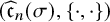 denote the Lie algebra with these generators and relations. Define a map from the set (5.8) to
$\mathfrak {c}_n(\sigma )$
 by
$d_{a,i,j;r} \mapsto e_{a,i,a,j}t^r, \ e_{a,i,j;r} \mapsto e_{a,i,a+1,j}t^r, \ f_{a,i,j;r} \mapsto e_{a+1,i, a,j} t^r$
 . One can easily verify using (5.7) that this extends to a surjective Lie algebra homomorphism
$\widehat {\mathfrak {c}}_n(\sigma ) \twoheadrightarrow \mathfrak {c}_n(\sigma )$
 . To show that this is an isomorphism it suffices to show that the elements

defined inductively by setting
$e_{a,i,a+1,j; r} := e_{a,i,j;r}$
 ,
$e_{a+1, i,a,j; r} := f_{a,i,j;r}$
 and


form a spanning set. Using (5.9),(5.11), (5.12) and a simple inductive argument one can see that
$\widehat {\mathfrak {c}}_n(\sigma )$
 is a direct sum of three subalgebras: the diagonal subalgebra, spanned by the elements
$d_{a,i,j;r}$
 , and the upper and lower triangular subalgebras
$^{\nu }\mathfrak {u}_n^+(\sigma )$
 and
$^{\nu }\mathfrak {u}_n^-(\sigma )$
 generated by the elements
$e_{a,i,j; r}$
 , respectively by the elements
$f_{a,i,j; r}$
 .
In order to complete the proof it suffices to show that
$\mathfrak {u}_n^+(\sigma )$
 and
$\mathfrak {u}_n^-(\sigma )$
 are spanned by the elements defined in (5.20) and (5.21) respectively. Since the argument is identical for
$\mathfrak {u}_n^+(\sigma )$
 and
$\mathfrak {u}_n^-(\sigma )$
 we only need to consider the former, where the claim follows from Lemma 5.1.
The Dirac reduced algebra in the following theorem should be viewed as a twisted shifted current Lie–Poisson algebra (see [Reference TopleyTo23, Remark 2.3]). Recall that for a shape
$\nu =(\nu _1, \dots , \nu _m)$
 and a four-tuple
$(a,i,b,j)\, 1 \le a,b \le m, \ 1 \le i \le \nu _a,\ 1 \le j \le \nu _b$
 we write
$(a,i',b,j'):=(a,\nu _a+1-i,b,\nu _b+1-j)$
 .
Theorem 5.3. If
$\beta = \pm 1$
 and
$\nu $
 is a
$(\beta , \sigma )$
 -admissible shape then
$S(\mathfrak {c}_n(\sigma ))$
 admits an involutive Poisson automorphism

The Dirac reduction
$R(S(\mathfrak {c}_n(\sigma )), \tau ) = S(\mathfrak {c}_n(\sigma )^\tau )$
 is Poisson generated by

subject to the relations


Proof. Relation (5.7) implies that
$\tau $
 gives a Poisson automorphism. By [Reference TopleyTo23, Remark 2.3] we can identify
$R(S(\mathfrak {c}_n(\sigma )), \tau )$
 with
$S(\mathfrak {c}_n(\sigma )^\tau )$
 , so it suffices to check that
$S(\mathfrak {c}_n(\sigma )^\tau )$
 has the stated Poisson presentation. Use [Reference TopleyTo23, (3.1)] to reduce the claim to a statement about the presentation of
$\mathfrak {c}_n(\sigma )^\tau $
 .
Consider the Lie algebra
$\widehat {\mathfrak {c}}_n(\sigma )^\tau $
 which is generated by the set (5.23) subject to relations (5.25)–(5.32). Make the notation
$\theta _{a,i,a+1,j}t^r := e_{a,i,a+1,j}t^r + \tau (e_{a,i,a+1,j}t^r), \ \eta _{a,i,a,j}t^r := e_{a,i,a,j}t^r + \tau (e_{a,i,a,j}t^r) \in \mathfrak {c}_n(\sigma )^\tau $
 . We define a map from the set (5.34) to
$\mathfrak {c}_n(\sigma )^\tau $
 by sending
$\eta _{a,i,j;r} \mapsto \eta _{a,i,a,j}t^{r} \in \mathfrak {c}_n(\sigma )^\tau $
 , and sending
$\theta _{a,i,j;r} \mapsto \theta _{a,i,a+1,j}t^r \in \mathfrak {c}_n(\sigma )^\tau $
 . One can check that this determines a surjective Lie algebra homomorphism
$\widehat {\mathfrak {c}}_n(\sigma )^\tau \twoheadrightarrow \mathfrak {c}_n(\sigma )^\tau $
 , indeed, checking that relations (5.25)–(5.32) hold amongst the corresponding elements of
$\mathfrak {c}_n(\sigma )^\tau $
 is a routine calculation using (5.7) and relation 5.24 follows immediately by definition of
$\tau $
 .
In order to complete the proof of (2) it is sufficient to show that this map is an isomorphism. This proof is similar to [Reference TopleyTo23, Theorem 3.3] but in our case there is a linear relation between the
$\eta _{a,i,j;r}$
 . For all admissible
$a,b,i,j,$
 and
$r \geq s_{a,b}$
 we inductively define elements

where
$\theta _{a,i,a+1,j;r} := \theta _{a,i,j;r}$
 . Let
$\{v_1, v_2,\dots \}$
 be a subset of
$\{\eta _{a,i,j;r} \mid 1 \le a \le m, \ 1 \le i,j \le \nu _{a}, \ r \geq 0 \}$
 such that it is a basis for the vector space spanned by
$\{\eta _{a,i,j;r} \mid 1 \le a \le m, \ 1 \le i,j \le \nu _{a}, \ r \geq 0 \}$
 together with the linear relation 5.24. It remains to check that
$\widehat {\mathfrak {c}}_n(\sigma )^\tau $
 is spanned by

We define a filtration
$\widehat {\mathfrak {c}}_n(\sigma )^\tau = \bigcup _{i> 0} \operatorname {F}_i \widehat {\mathfrak {c}}_n(\sigma )^\tau $
 by placing the generators (5.23) in degree 1 and satisfying
$\operatorname {F}_{d} \widehat {\mathfrak {c}}_n(\sigma )^\tau = \sum _{d_1 + d_2 = d} \{\operatorname {F}_{d_1} \widehat {\mathfrak {c}}_n(\sigma )^\tau , \operatorname {F}_{d_2} \widehat {\mathfrak {c}}_n(\sigma )^\tau \}$
 . By convention
$\operatorname {F}_{0} \widehat {\mathfrak {c}}_n(\sigma )^\tau = 0$
 . The associated graded Lie algebra
$\operatorname {gr} \widehat {\mathfrak {c}}_n(\sigma )^\tau = \bigoplus _{i> 0} \operatorname {F}_i \widehat {\mathfrak {c}}_n(\sigma )^\tau / \operatorname {F}_{i-1} \widehat {\mathfrak {c}}_n(\sigma )^\tau $
 is generated by elements


These generators of
$\operatorname {gr} \widehat {\mathfrak {c}}_n(\sigma )^\tau $
 satisfy the top graded components of the relations (5.24)–(5.32).
Let
$\mathfrak {a}$
 be an abelian Lie algebra with spanning set
$\{d_{a,i,j} t^r \mid 1\le a \le m, \ 1 \le i,j \le \nu _{a}, \ 0 \leq r\}$
 and relations
$d_{a,i,j} t^r=(\beta )^{i+j}(-1)^{r-1}d_{a,\nu _a+1-j,\nu _a+1-i}$
 . Let
$\mathfrak {u}_n(\sigma )$
 be the Lie subalgebra of
$\mathfrak {c}_n(\sigma )$
 described in Lemma 5.1. Then
$\mathfrak {a} \oplus \mathfrak {u}_n(\sigma )$
 is a Lie algebra with
$\mathfrak {a}$
 an abelian ideal. Comparing the top components (5.24)–(5.32) to (5.4)–(5.6) we see that there is a surjective Lie algebra homomorphism
$\mathfrak {a} \oplus \mathfrak {u}_n(\sigma ) \twoheadrightarrow \operatorname {gr} \widehat {\mathfrak {c}}_n(\sigma )^\tau $
 defined by
$d_{a,i,j} t^{r} \mapsto \overline {\eta }_{a,i,j; r}$
 and
$e_{a,i,a+1,j}t^r \mapsto \overline {\theta }_{a,i,j;r}$
 . The algebra
$\mathfrak {a} \oplus \mathfrak {u}_n(\sigma )$
 has basis consisting of elements
$e_{a,h,b,k}t^s$
 where
$ 1\le a < b \le m, 1 \le h \le \nu _{a}, \ 1 \le k \le \nu _{b}, \ s \ge s_{a,b}$
 together with a basis
$\{w_1,w_2,\dots \}$
 for the vector space
$\mathfrak {a}$
 which can be picked such that
$w_1 \mapsto v_1$
 . It follows that
$\operatorname {gr} \widehat {\mathfrak {c}}_n(\sigma )^\tau $
 is spanned by elements
$\overline {v_1},\overline {v_2},\dots , \overline {\theta }_{a,i,b,j;s}$
 where the indices vary in the ranges specified in (5.34), and
$\overline {\theta }_{a,i,b,j;s}$
 defined inductively from (5.36), analogously to (5.33). We deduce that
$\widehat {\mathfrak {c}}_n(\sigma )^\tau $
 is spanned by the required elements, which completes the proof.
Remark 5.4. It is crucial for this theorem that our shape
$\nu $
 is
$(\beta ,\sigma )$
 -admissible, otherwise
$\tau $
 is not an involution.
Our next result, which we record here for later use, explains the relationship between the shifted current algebras and the centralisers described above.
Lemma 5.5. Let
$\varepsilon = \pm 1$
 and
$N> 0$
 such that
$\varepsilon ^N = 1$
 . Let
$\lambda \in \mathcal {P}_\varepsilon (N)$
 be an even partition, and let
$\sigma $
 be the shift matrix determined by
$\lambda $
 , as in Lemma 2.1. Let
$\beta =-\varepsilon (-1)^{\lambda _1}$
 and pick a
$(\beta , \sigma )$
 -admissible shape and let
$\tau : \mathfrak {c}_n(\sigma ) \to \mathfrak {c}_n(\sigma )$
 be the involution (5.22). Abusing notation we also write
$\tau : \mathfrak {gl}_N \to \mathfrak {gl}_N$
 for the automorphism described in (4.10).
-
(1) There is a surjective Lie algebra homomorphism
$$ \begin{align*} \mathfrak{c}_n(\sigma) & \twoheadrightarrow \mathfrak{gl}_N^e \\e_{a,i,b,j}t^r & \longmapsto c_{a,i,b,j}^{(r)} \end{align*} $$where $c_{a,i,b,j}^{(r)} := 0$
for
$r \ge s_{a,b} + \min (\lambda _a, \lambda _b)$
. The kernel is Poisson generated by
$e_{1,i,1,j}t^r$
with
$r\ge \lambda _1$
,
$1 \leq i,j \leq \nu _{1}$
-
(2) The homomorphism from (1) restricts to $\mathfrak {c}_n(\sigma )^\tau \twoheadrightarrow (\mathfrak {g}^e)^\tau $
.-
(i) For $\varepsilon =1$
the kernel is generated as a Lie ideal by (5.37) $$ \begin{align} \{\eta_{1,i,j;r} \mid r \ge \lambda_1 \ , 1 \le i,j \le \nu_1\} \end{align} $$
-
(ii) For $\varepsilon = -1$
and
$\nu _1\ne 1$
the kernel is generated by (5.37) -
(iii) For $\varepsilon =-1$
and
$\nu _1 = 1$
the kernel is generated by those elements, along with (5.38) $$ \begin{align} \{\theta_{1,i,j; \lambda_1 + s_{1,2}} \mid 1\le i \le \nu_1 , \ 1 \le j \le \nu_{2} \}. \end{align} $$
-









Proof. Part (1) is essentially the same as [Reference Goodwin and TopleyGT19c, Lemma 2.6].
Compare (5.22) with Lemma 4.2(iii) to see that the map is
$\tau $
 -equivariant, hence it is a well-defined map
$\mathfrak {c}_n(\sigma )^\tau \twoheadrightarrow (\mathfrak {g}^e)^\tau $
 .
We go on to describe the kernel in (2). First of all observe that the elements listed there are
$\tau $
 -fixed elements of the kernel of
$\mathfrak {c}_n(\sigma )\twoheadrightarrow \mathfrak {g}^e$
 . Now observe that
$\mathfrak {g}_0^e$
 has a spanning set consisting of elements of the form
$c_{a,i,b,j}^{(r)} + \tau (c_{a,i,b,j}^{(r)})$
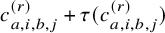 . By Lemma 4.1 we can show that the elements in (2) generate the kernel by checking that the ideal
$\mathfrak {i}$
 which they generate contains

Consider the case
$\epsilon = 1$
 in (2)(i) and note that in this case for each i there is a j such that we have
$\eta _{1,i,j;\lambda _1} \neq 0$
 . This is obvious if
$\nu _1 \neq 1$
 whereas if
$\nu _1=1$
 we have that
$\lambda _1$
 is odd by
$(\beta , \sigma )$
 admissibility as
$\beta =-\varepsilon (-1)^{\lambda _1}$
 and hence
$\eta _{1,1,1,\lambda _{1}}=d_{1,1,1,\lambda _{1}}+(-1)^{\lambda _1-1}d_{1,1,1,\lambda _{1}} \neq 0$
 . Using relation (5.26) we see that
$\mathfrak {i}$
 contains
$\{\eta _{1,i,j;\lambda _1}, \theta _{1,j,k;r}\} = \theta _{1,i,k; \lambda _1 + r}$
 for
$r \ge s_{1,2}$
 and all admissible
$i,k$
 whilst (5.28) together with the fact that
$\eta _{1,i,j,\lambda _2+r} \in \mathfrak {i}$
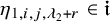 for
$r \geq 0$
 shows that
$\eta _{2,i,j;\lambda _2+r} \in \mathfrak {i}$
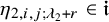 for
$r\ge 0$
 and all admissible
$i,j$
 . By Theorem 5.3 the subalgebra of
$\mathfrak {c}_n(\sigma )^\tau $
 generated by
$\eta _{a,i,j;r}, \theta _{a,i,j;r}$
 with
$2\le a$
 is isomorphic to a current Lie algebra associated with a lower rank general linear Lie algebra and a shape of strictly smaller length. The description of the kernel follows by induction.
In the second case we see that if
$\nu _1 \neq 1$
 for each i there is some j such that
$\eta _{1,i,j;\lambda _1}\neq 0$
 . Hence the ideal
$\mathfrak {i}$
 contains
$\{\eta _{1,i,j;\lambda _1}, \theta _{1,j,k; s}\} = \theta _{1,i,k;\lambda _1+s}$
 for
$s \ge s_{1,2}$
 , proving (ii).
If
$\nu _1=1$
 we see that
$\eta _{1,1,1;\lambda _1+1} \neq 0$
 . Hence the ideal
$\mathfrak {i}$
 contains
$\{\eta _{1,1,1;\lambda _1+1}, \theta _{1,1,k; s}\} = \theta _{1,1,k;\lambda _1 + 1 + s}$
 for
$s \ge s_{1,2}$
 . Together with the additional generators
$\theta _{1,i,j;\lambda _1 + s_{1,2}}$
 this gives all elements of the form
$\theta _{1,i,j;r}$
 listed in (5.39).
Furthermore if
$\nu _1=1$
 we have by
$(\beta , \sigma )$
 admissibility that
$\lambda _1$
 is even. In particular by (5.32) we have that we have

as we have
$\lambda _2=\lambda _1+2s_{1,2}$
 . So all additional generators of the form
$\theta _{2,i,j;\lambda _2 + s_{2,3}}$
 also lie in the ideal. Now the inductive proof of (iii) proceeds in the same way as in the first case.
5.2 The semiclassical shifted Yangian
In this section we fix
$n> 0$
 , an
$n\times n$
 shift matrix
$\sigma $
 and a
$\sigma $
 -admissible shape
$\nu $
 . The (semiclassical) shifted Yangian with respect to an admissible shape
$^{\nu }y_n(\sigma )$
 is the Poisson algebra generated by the set

together with relations


for all admissible
$a,b,f,g,h,i,j,k,r,s,t$
 . In these relations we use the notation
$d_{a,i,j}^{(0)}=\widetilde {d}_{a,i,j}^{(0)}=\delta _{i,j}$
 and define
$\widetilde {d}_{a,i,j}^{(r)}$
 recursively.

In order to describe the structure of
$^{\nu }y_n(\sigma )$
 as a commutative algebra we make the notation


and inductively define


For
$1 \leq k \leq \nu _{b-1}$
 note that by the relations this is independent of the choice of k see [Reference Brundan and KleshchevBK06, 3.16]. The shifted Yangian admits a Poisson grading
$^{\nu }y_n(\sigma ) = \bigoplus _{r \ge 0} {}^{\nu }y_n(\sigma )_r$
 , which we call the canonical grading. It places
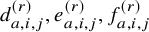
$d_{a,i,j}^{(r)}, e_{a,i,j}^{(r)}, f_{a,i,j}^{(r)}$
 in degree r and the bracket lies in degree
$-1$
 , meaning
$\{\cdot , \cdot \} : \ ^{\nu }y_n(\sigma )_r \times \ ^{\nu }y_n(\sigma )_s \to \ ^{\nu }y_n(\sigma )_{r+s-1}$
 . There is also an important Poisson filtration
$^{\nu }y_n(\sigma ) = \bigcup _{i \ge 0} \operatorname {F}_i \ ^{\nu }y_n(\sigma )$
 , called the loop filtration, defined by placing
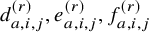
$d_{a,i,j}^{(r)}, e_{a,i,j}^{(r)}, f_{a,i,j}^{(r)}$
 in degree
$r-1$
 . With respect to this filtration, the bracket is in degree zero so that
$\operatorname {F}_r y_n(\sigma ) \times \operatorname {F}_s y_n(\sigma ) \to \operatorname {F}_{r+s}y_n(\sigma )$
 . The associated graded Poisson algebra is denoted
$\operatorname {gr} y_n(\sigma )$
 .
The following theorem is a semiclassical analogue of [Reference Brundan and KleshchevBK06, Theorem 2.1], which we ultimately deduce from the noncommutative setting, analogous to [Reference TopleyTo23, Theorem 3.4].
Theorem 5.6. Let
$\sigma $
 be a symmetric shift matrix and
$\nu $
 a
$\sigma $
 -admissible shape. There is a Poisson isomorphism
$S(\mathfrak {c}_n(\sigma )) \overset {\sim }{\longrightarrow } \operatorname {gr} \ ^{\nu }y_n(\sigma )$
 defined by

As a consequence
$y_n(\sigma )$
 is isomorphic to the polynomial algebra on infinitely many variables

Proof. Comparing the top graded components of the relations (5.41)–(5.52) with respect to the loop filtration, with relations (5.9)–(5.18), it is straightforward to see that (5.58) gives a surjective Poisson homomorphism. To prove the theorem we demonstrate that the ordered monomials in the elements (5.59) are linearly independent.
Consider the set

In [Reference Brundan and KleshchevBK06, §3] the shifted Yangian
$^{\nu }Y_n(\sigma )$
 is defined as a quotient of the free algebra
$\mathbb {C}\langle X \rangle $
 by the ideal generated by the relations [Reference Brundan and KleshchevBK06, (3.3)–(3.14)]. Let
$L := L_X$
 be the free Lie algebra on X and define a grading
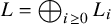
$L = \bigoplus _{i \ge 0} L_i$
 by placing
$E_{a,i,j}^{(r)}, F_{a,i,j}^{(r)}, D_{a,i,j}^{(r)}$
 in degree
$r-1$
 . Then we place a filtration on the enveloping algebra
$U(L)$
 so that
$L_i$
 lies in degree
$i+1$
 . By the PBW theorem for
$U(L)$
 we see that
$\operatorname {gr} U(L) \cong S(L)$
 .
The universal property of
$U(L)$
 ensures that there is a surjective algebra homomorphism
$U(L) \twoheadrightarrow \mathbb {C}\langle X \rangle $
 and by [Reference SerreSer06, I, Ch. IV, Theorem 4.2] this is an isomorphism. Identifying these algebras, the filtration on
$U(L)$
 descends to
$^{\nu }Y_n(\sigma ) = \bigcup _{i\ge 0} \operatorname {F}^{\prime }_i \, {}^{\nu }Y_n(\sigma )$
 , and this resulting filtration is commonly referred to as the canonical filtration [Reference Brundan and KleshchevBK06, §5]. The associated graded algebra
$\operatorname {gr} {}^{\nu }Y_n(\sigma )$
 is equipped with a Poisson structure in the usual manner. Comparing relations (5.41)–(5.52) with the top graded components of relations [Reference Brundan and KleshchevBK06, (3.3)–(3.14)] we see that the Poisson surjection
$S(L) \twoheadrightarrow \operatorname {gr} {}^{\nu }Y_n(\sigma )$
 factors through
$S(L) \to {}^{\nu }y_n(\sigma )$
 . As a result there is a surjective Poisson homomorphism
$\pi : {}^{\nu }y_n(\sigma ) \twoheadrightarrow \operatorname {gr} {}^{\nu }Y_n(\sigma )$
 given by
$e_{a,i,j}^{(r)} \mapsto E_{a,i,j}^{(r)} + \operatorname {F}^{\prime }_{r-1} {}^{\nu }Y_n(\sigma ), f_{a,i,j}^{(r)} \mapsto F_{a,i,j}^{(r)} + \operatorname {F}^{\prime }_{r-1} {}^{\nu }Y_n(\sigma ), d_{a,i,j}^{(r)} \mapsto D_{a,i,j}^{(r)} + \operatorname {F}^{\prime }_{r-1} {}^{\nu }Y_n(\sigma )$
 . Following [Reference Brundan and KleshchevBK06, (3.15), (3.16)] we introduce elements
$E_{a,i,b,j}^{(r)}, F_{a,i,b,j}^{(r)}$
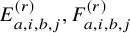 of
$^{\nu }Y_n(\sigma )$
 lying in filtered degree r. By the definition of the filtration and the elements (5.56), (5.57) we have

By [Reference Brundan and KleshchevBK06, Theorem 3.2(iv)] the ordered monomials in
$E_{a,i,b,j}^{(r)}, F_{a,i,b,j}^{(r)}, D_{a,i,j}^{(r)}$
 are linearly independent in
$^{\nu }Y_n(\sigma )$
 and so we deduce that the images of these monomials in
$\operatorname {gr} ^{\nu }Y_n(\sigma )$
 are linearly independent. This completes the proof.
We record two formulas for future use.
Lemma 5.7. The following hold for
$i=1,...,n$
 ,
$j = 1,...,n-1$
 ,
$r> 0$
 and
$s> s_{j,j+1}$
 :


Proof. We only sketch (5.61), as the proof of (5.62) is almost identical. The argument is by induction based on (5.53). Note that
$\widetilde {d}_{a,i,j}^{(1)} = -d_{a,i,j}^{(1)}, \widetilde {d}^{(0)}_{a,i,j}=d^{(0)}_{a,i,j}=\delta _{i,j}$
 and so (5.61) is equivalent to (5.43) in this case. We have
$\{\widetilde {d}_{a,i,j}^{(r)}, e_{b,h,k}^{(s)}\} = \{-\sum _{g=1}^{\nu _a}\sum _{t=1}^{r} d_{a,i,g}^{(t)} \widetilde {d}_{a,g,j}^{(r-t)}, e_{b,h,k}^{(s)}\}$
 and relation (5.43) together with the inductive hypothesis imply that the coefficient of
$e_{b,m,n}^{(s+t)}$
 is

Using
$d_{a,i,j}^{(0)} = \widetilde {d}_{a,i,j}^{(0)} = \delta _{i,j}$
 we see that all quadratic terms cancel, whilst the linear term equates to
$\delta _{a,b+1}\delta _{m,h}\widetilde {d}_{a,n,j}^{(r-t-1)}\delta _{i,k} - \delta _{a,b}\delta _{n,k} \delta _{i,m}\widetilde {d}_{a,h,j}^{(r-t-1)}$
 , which concludes the induction.
5.3 The Dirac reduction of the shifted Yangian
In this section we suppose that
$\sigma $
 is symmetric and we let
$\nu =(\nu _1,\dots , \nu _m)$
 be a
$(\beta ,\sigma )$
 -admissible shape. Examining the relations (5.41)–(5.52) we see that there is unique involutive Poisson automorphism
$\tau $
 of
$y_n(\sigma )$
 determined by

Remark 5.8. Note that for this automorphism to be involutive we need
$\nu $
 to be
$(\beta ,\sigma )$
 -admissible and that the automorphism
$\tau $
 depends on the shape.
Our present goal is to give a complete description of the Dirac reduction
$R(^{\nu }y_n(\sigma ), \tau )$
 . Before doing so we will state the relationship between
$R(^{\nu }y_n(\sigma ), \tau )$
 ,
$R(^{\mu }y_n(\sigma ), \tau )$
 where both
$\mu $
 and
$\nu $
 are
$(\beta ,\sigma )$
 -admissble.
Proposition 5.9. Let
$\nu $
 ,
$\mu $
 be
$(\beta , \sigma )$
 -admissible shapes. Denote by
${}^{\nu }\tau $
 ,
${}^{\mu }\tau $
 the involutions on
$^{\nu }y_n(\sigma )$
 ,
$^{\mu }y_n(\sigma )$
 as defined in (5.63). Then there exists a
$\mathbb {Z}/2$
 -equivariant isomorphism

where the
$\mathbb {Z}/2$
 -action on the left is given by
${}^\nu \tau $
 and on the right by
${}^\mu \tau $
 .
Proof. We will prove the result for
$GL_{\mu _1} \times \dots \times GL_{\mu _m} \subseteq GL_{\nu _1} \times \dots \times GL_{\nu _{m'}}$
 . This suffices as for
$\beta =1$
 the shape
$(1,1,\dots ,1,1)$
 is always
$(1,\sigma )$
 -admissible and if
$\sigma $
 admits a
$\beta =-1$
 admissible shape then the shape
$(2,2,\dots ,2,2)$
 is always
$(-1,\sigma )$
 -admissible. The general result then follows by composing isomorphisms. Let
${}^{\nu }Y_n(\sigma )$
 denote the shifted Yangian of shape
$\nu $
 as defined in [Reference Brundan and KleshchevBK06, §3]. Also write
$Y_n$
 for the Yangian for
$\mathfrak {gl}_n$
 . Recall the definition of parabolic presentations of
$Y_n$
 from [Reference Brundan and KleshchevBK05, §6] where the elements
$E_{a,b,i,j}^{(r)},F_{a,b,i,j}^{(r)},D_{a,i,j}^{(r)}$
 are defined in terms of a Gauss decomposition of the T-matrix or more explicitly by quasi determinants [Reference Brundan and KleshchevBK05, (6.2)-(6.4)]. By [Reference Brundan and KleshchevBK06, Corollary 3.3] the canonical map
$i_{\nu }:{}^{\nu }Y_n(\sigma ) \to Y_n$
 given by sending the generators to the elements with the same name is injective and its image is independent of the choice of
$\nu $
 . Furthermore by [Reference Brundan and KleshchevBK05, §5] the map is filtered with respect to the canonical filtration. Consider now the map
$\tau _{\nu }:Y_n \to Y_n: T(u) \mapsto J_{\nu }^{-1}T(-u)^tJ_{\nu }$
 where

By [Reference MolevMo07, §1.3] this is an automorphism. Note that
$J_{\nu }$
 is a block diagonal matrix that can be described as follows. For each index
$a = 1,...,m$
 there is a block of size
$\nu _a$
 , each of these blocks has entries
$(-1)^{s_{1,a}(\nu )}$
 on the antidiagonal and zeros elsewhere when
$\beta =1$
 . When
$\beta =-1$
 it has alternating entries
$(-1)^{s_{1,a}(\nu )}(\mp 1)$
 on the antidiagonal and zeroes elsewhere. Thus when
$\beta = 1$
 the matrix J is a block diagonal matrix where each block is symmetric and when
$\beta = -1$
 each block is antisymmetric. It follows that

We claim that


and in particular the image of
$i_{\nu }$
 is stabilised by
$\tau _{\nu }$
 . Indeed by [Reference Brundan and KleshchevBK05, (6.6)-(6.8)] we have that for the automorphism
$\omega :Y_n \to Y_n: T(u) \mapsto T(-u)^\top $


Furthermore using the explicit description of
$E_{a,a+1,i,j}^{(r)}$
 ,
$F_{a+1,a,i,j}^{(r)}$
 ,
$D_{a,a,i,j}^{(r)}$
 in terms of quasi determinants and [Reference Gelfand, Gelfand, Retakh and WilsonGGRW04, §1.3(i),(ii)] it follows immediately that for any matrix
$A=(A_{\nu _1}, \dots , A_{\nu _m}) \in GL_{\nu _1} \times \cdots \times GL_{\nu _m}$
 and for the automorphism given by
$c_A:T(u) \mapsto A^{-1}T(u)A$
 we have

where
$(E_{a,a+1}^{(r)})_{i,j}=E_{a,a+1,i,j}^{(r)}$
 ,
$(F_{a+1,a}^{(r)})_{i,j}=F_{a+1,a,i,j}^{(r)}\, (D_{a,a}^{(r)})_{i,j}=D_{a,a,i,j}^{(r)}$
 . The claim then follows by direct calculation.
From the description of the matrices
$J_{\nu }$
 and
$J_{\mu }$
 it follows that there exists
$B \in GL_{\nu _1} \times \dots \times GL_{\nu _m}$
 such that
$J_{\mu }=B^{t}J_{\nu }B$
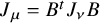 . It follows from (5.70) that the automorphism
$c_{B}:Y_n \to Y_n : T(u) \mapsto B^{-1}T(u)B$
 stabilises the image of
$i_{\nu }$
 and that it is filtered with respect to the canonical filtration as defined in [Reference Brundan and KleshchevBK06, §5]. It thus follows that
$i_{\mu }^{-1} \circ c_{B} \circ i_{\nu }:{}^{\nu }Y_n(\sigma ) \to {}^{\mu }Y_n(\sigma ) $
 is well defined and filtered.
Recall from the proof of Theorem 5.6 that the map
$\pi _{\nu }: {}^{\nu }y_n(\sigma ) \twoheadrightarrow \operatorname {gr} \ ^{\nu }Y_n(\sigma )$
 given by
$e_{a,i,j}^{(r)} \mapsto E_{a,i,j}^{(r)} + \operatorname {F}^{\prime }_{r-1} \ ^{\nu }Y_n(\sigma ), f_{a,i,j}^{(r)} \mapsto F_{a,i,j}^{(r)} + \operatorname {F}^{\prime }_{r-1} \ ^{\nu }Y_n(\sigma ), d_{a,i,j}^{(r)} \mapsto D_{a,i,j}^{(r)} + \operatorname {F}^{\prime }_{r-1} \ ^{\nu }Y_n(\sigma )$
 is an isomorphism of Poisson algebras, where
$\operatorname {F}'$
 denotes the canonical filtration. In particular
$\pi _{\mu }^{-1} \circ \operatorname {gr}( i_{\mu }^{-1} \circ c_{B} \circ i_{\nu }) \circ \pi _{\nu }$
 is the desired isomorphism.
Corollary 5.10. Let
$\nu $
 ,
$\mu $
 be
$(\beta , \sigma )$
 -admissible shapes. Then the Dirac reductions
$R({}^{\nu }y_n(\sigma ), {}^{\nu }\tau )$
 and
$R({}^{\mu }y_n(\sigma ), {}^{\mu }\tau )$
 are Poisson isomorphic.
Remark 5.11. The proof of Theorem B now follows by combining Corollary 5.10 with Theorem 3.9 which is the special case for
$\mu =(1,1,\dots ,1,1)$
 , stating that
$y_n^+(\sigma ) \cong R({}^{\mu }y_n(\sigma ),\tau )$
 . The parabolic presentations of
$y_n^+(\sigma )$
 alluded to in Theorem B are actually the parabolic presentations
$R(^{\nu }y_n(\sigma ),\tau )$
 which are formulated in Theorem 5.13.
For all admissible
$a,i,j,r$
 we write

Remark 5.12. Compare (5.71) with [Reference TopleyTo23, (3.59)] to see that in the case
$\nu =(1,1,\dots ,1,1)$
 we have
$\widehat {d}_{i,1,1}^{(r)}=\widehat {d}_{i}^{(r)}$
 and
$\widehat {e}_{i,1,1}^{(r)}= \frac {1}{2} \widehat {e}_{i}^{(r)}$
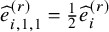 .
Now let
$\check{y}_n(\sigma )$
 be the ideal of
$y_n(\sigma )$
 generated by

for all admissible
$a,i,j,b,h,k,r,s$
 . Also write
$\check{y}_n(\sigma )^\tau := \check{y}_n(\sigma ) \cap y_n(\sigma )^\tau $
 . By [Reference TopleyTo23, Lemma 2.2] we see that
$R(^{\nu }y_n(\sigma ), \tau ) = ^{\nu }y_n(\sigma )^\tau / ^{\nu }\check{y}_n(\sigma )^\tau $
 is Poisson generated by elements

with Poisson brackets induced by the bracket on
$y_n(\sigma )$
 . We will write
$\theta _{a,i,j}^{(r)}$
 ,
$\eta _{a,i,j}^{(r)}$
 for
$ \widehat {e}_{a,i,j}^{(r)} + \check{y}_n(\sigma )^\tau $
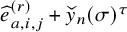 and
$\widehat {d}_{a,i,j}^{(r)} + \check{y}_n(\sigma )^\tau $
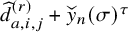 . Furthermore
$R(^{\nu }y_n(\sigma ), \tau )$
 is generated as a commutative algebra by elements

where
$\theta _{a,i,b,j}^{(r)} := e_{a,i,b,j}^{(r)} +(\beta )^{i+j} (-1)^{r+s_{a,b}} f_{a,j',b,i'}^{(r)}$
 . Using an inductive argument and (5.42) we see the elements
$\theta _{a,i,b,j}^{(r)}$
 can also be defined via the following recursion for all admissible
$a,b,i,j,r$
 .

Thanks to Theorem 5.6 we see that
$R(y_n(\sigma ), \tau )$
 comes equipped with the canonical grading
$R(y_n(\sigma ), \tau ) = \bigoplus _{i \ge 0} R(y_n(\sigma ), \tau )_i$
 which places
$\eta _{a,i,j}^{(r)}, \theta _{a,i,j}^{(r)}$
 in degree r and the Poisson bracket in degree
$-1$
 . Another crucial feature is the loop filtration
$R(y_n(\sigma ), \tau ) = \bigcup _{i\ge 0} \operatorname {F}_iR(y_n(\sigma ), \tau )$
 which places
$\eta _{a,i,j}^{(r)}, \theta _{a,i,j}^{(r)}$
 in degree
$r-1$
 and the bracket in degree
$0$
 . Both of these structures are naturally inherited from
$y_n(\sigma )$
 .
The following is our main structural result on the Dirac reduction of the shifted Yangian.
Theorem 5.13.
$R(^{\nu }y_n({\sigma }),\tau )$
 is Poisson generated by

with the following Poisson relations


Here we define
$\eta _{a,i,j}^{(0)}=\delta _{i,j}$
 ,
$\widetilde {\eta }_{a,i,j}^{(0)}=\delta _{i,j}$
 and
$\widetilde {\eta }_{a,i,j}^{(r)}=-\sum _{g=1}^{\nu _a} \sum _{t=1}^{r} \eta _{a,i,g}^{(t)} \tilde {\eta }_{a,g,j}^{(r-t)}$

Proof. In this proof we will frequently use the following two basic facts:
$(\beta )^{i+j}=(\beta )^{i'+j'}$
 , which follows from
$(\beta , \sigma )$
 -admissibility, and
$xy+\tau (xy)=\frac {1}{2}(x+\tau (x))(y+\tau (y))$
 for any
$x,y \in R(y_n(\sigma ),\tau )$
 .
First note that
$\widetilde {\eta }_{a,i,j}^{(r)}=\frac {1}{2}(\tilde {d}_{a,i,j}^{(r)}+\tau (\tilde {d}_{a,i,j}^{(r)}))$
 . The proof is by induction on r

Relation (5.76) follows immediately. For relation (5.77) we have

Using relation (5.41). For relation (5.78) we have

Using relations (5.43) and (5.44). For
$r<s$
 we have

Where we used relations (5.42), (5.45) and (5.46). The next relation follows from using relations (5.42), (5.47) and (5.48).

Finally the last relation follows from using relations (5.42), (5.51), (5.52), (5.43), (5.44) and Lemma 5.7.

If
$r+s$
 is odd then this vanishes whereas if
$r+s$
 is even this simplifies too

Let
$\widehat {R}(^{\nu }y_n(\sigma ), \tau )$
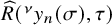 denote the Poisson algebra with generators (5.75) and relations (5.76)-(5.83). We have shown that there is a surjection
$\widehat {R}(^{\nu }y_n(\sigma ), \tau ) \twoheadrightarrow {R}(^{\nu }y_n(\sigma ), \tau ) $
 . To conclude the proof we show that it sends a spanning set to a basis. We define a loop filtration on
$\widehat {R}(^{\nu }y_n(\sigma ), \tau )=\bigcup _{i \geq 0}F_{i}\widehat {R}(^{\nu }y_n(\sigma ), \tau )$
 by placing the generators
$\theta _{a,i,j}^{(r)}, \eta _{a,i,j}^{(r)}$
 in degree
$r-1$
 and the bracket in degree 0.
Examining the top filtered components of (5.77)-(5.83) we see from Theorem 5.3 that there is a surjective Poisson morphism
$R(S(\mathfrak {c}_n(\sigma )), \tau ) \twoheadrightarrow \operatorname {gr} \widehat {R}(^{\nu }y_n(\sigma ), \tau ) $
 . We thus see that
$\operatorname {gr} \widehat {R}(^{\nu }y_n(\sigma ), \tau )$
 is generated as a commutative algebra by the elements
$\eta _{a,i,j}^{(r)}+F_{r-2}\widehat {R}(^{\nu }y_n(\sigma ), \tau ),\theta _{a,i,b,j}^{(r)}+F_{r-2}\widehat {R}(^{\nu }y_n(\sigma ), \tau )$
 which are again defined via the recursion (5.74).
By a standard filtered algebra argument
$ \widehat {R}(^{\nu }y_n(\sigma ), \tau )$
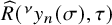 is generated as a commutative algebra by the elements with the same names in
$\operatorname {gr} \widehat {R}(^{\nu }y_n(\sigma ), \tau )$
 . We have thus shown that
$\widehat {R}(^{\nu }y_n(\sigma ), \tau ) \twoheadrightarrow {R}(^{\nu }y_n(\sigma ), \tau ) $
 maps a spanning set to a basis, which concludes the proof.
Remark 5.14. Strictly speaking we need to take care of the linear relations (5.76) between the
$\eta _{a,i,j}^{(r)}$
 to conclude that a spanning set gets sent to a basis. This can be dealt with in exactly the same way as the proof of Theorem 5.3.
Remark 5.15. Note that [Reference TopleyTo23, Theorem 3.7] is a special case of this presentation where
$\nu =(1,1,\dots ,1,1)$
 , the only difference being in scaling due to a different convention of the scaling of generators as explained in Remark 5.12.
Let
$\operatorname {gr} R(y_n(\sigma ), \tau )$
 denote the graded algebra for the loop filtration. In the last paragraph of the proof of Theorem 5.13 we obtained the following important result.
Corollary 5.16. If
$\sigma $
 is a symmetric shift matrix and
$^{\nu }y_n(\sigma )$
 is the semiclassical shifted Yangian then there is an isomorphism of commutative algebras
$S(^{\nu }\mathfrak {c}_n(\sigma )^\tau ) \overset {\sim }{\longrightarrow } \operatorname {gr} R(^{\nu }y_n(\sigma ), \tau )$
 given by

6 The Dirac reduced semiclassical Brundan–Kleshchev homomorphism
6.1 The semiclassical Brundan–Kleshchev homorphism
Fix
$\varepsilon = \pm 1$
 and an integer
$N> 0$
 such that
$\varepsilon ^N = 1$
 . Let
$\lambda = (\lambda _1 \le \lambda _2 \le \cdots \le \lambda _n) \in \mathcal {P}_\varepsilon (N)$
 be a partition associated with all parts of the same parity. Following Section 4.1 we choose a nilpotent element
$e\in \mathfrak {gl}_N$
 with Jordan blocks of size
$\lambda _1,...,\lambda _n$
 , and an involution
$\tau : \mathfrak {gl}_N \to \mathfrak {gl}_N$
 such that the fixed point subalgebra
$\mathfrak {g} = \mathfrak {gl}_N^\tau $
 is simple of type

Since
$\tau $
 fixes the
$\mathfrak {sl}_2$
 -triple
$(e,h,f)$
 it also stabilises the slice
$e + \mathfrak {gl}_N^f$
 and acts by Poisson automorphisms on
$S(\mathfrak {gl}_N,e)$
 .
Now let
$(\sigma , \ell )$
 be the
$n\times n$
 shift matrix and the level determined by
$\lambda $
 as in (2.1). We pick a
$(-\varepsilon (-1)^{\lambda _1}, \sigma )$
 -admissible shape and by slight abuse of notation we also let
$\tau $
 denote the automorphism of
$^\nu y_n(\sigma )$
 described in (5.63).
Theorem 6.1. There is a
$\tau $
 -equivariant surjective Poisson homomorphism
$^\nu y_n(\sigma ) \to S(\mathfrak {g},e)$
 determined by

The kernel is generated as a Poisson ideal by

Proof. The existence of the homomorphism from the shifted Yangian to the quantum finite W-algebra is proven by Brundan and Kleshchev in [Reference Brundan and KleshchevBK06, Theorem 10.1]. The result stated here follows from theirs by taking the associated graded algebras with respect to the canonical filtration and the Kazhdan filtration. The
$\tau $
 -equivariance follows by comparing Proposition 4.5 with formula (5.63).
The fact that the elements (6.1) lie in the kernel of the map is an immediate consequence of [Reference Brundan and KleshchevBK06, Theorem 10.1]. The fact that these elements generate the kernel can be proven using an argument identical to [Reference TopleyTo23, Proposition 4.7], deploying our Lemma 5.5(1).
6.2 Dirac reduction of the homomorphism
We now proceed to introduce an element of
$y_n(\sigma )^\tau $
 which lies in the kernel of the map appearing in Theorem 6.1, which deforms the element (5.38) via the loop filtration.
To do so first let
$\dot {d}_{1,i,j}^{(\lambda _1(\nu )+1)} := \check{d}_{1,i,j}^{(\lambda _1(\nu )+1)} \in \ ^{\nu }y_n(\sigma )$
 Note that
$\tau (\dot {d}_{1,i,j}^{(\lambda _1(\nu )+1)}) = -\dot {d}_{1,i,j}^{(\lambda _1(\nu )+1)}.$
 Therefore we may define

Theorem 6.2. There is a surjective Poisson homomorphism
$\varphi :R(^\nu y_n(\sigma ), \tau ) \twoheadrightarrow S(\mathfrak {g}_0, e)$
 .
-
(i) When $\varepsilon =1$
, the kernel is Poisson generated by (6.3) $$ \begin{align} \{\eta_{1,i,j}^{(r)} \mid r> \lambda_1(\nu) \ , 1 \le i,j \le \nu_1\}. \end{align} $$
-
(ii) When $\varepsilon =-1$
and
$\nu _1 \ne 1$
the kernel is Poisson generated by (6.3) -
(iii) When $\varepsilon = -1$
and
$\nu _1 = 1$
the kernel is Poisson generated by those same elements, along with (6.4) $$ \begin{align} \{\dot{\theta}_{1,i,j}^{( \lambda_1(\nu) + s_{1,2}(\nu)+1)} \mid 1\le i , \le \nu_1 \ , 1 \le j \le \nu_{2} \}. \end{align} $$


Proof. The existence of this surjective map follows by [Reference TopleyTo23, (2.6) &Theorem 2.6] and Theorem 6.1. For the kernel consider first the case (i). It follows from Theorem 6.1 that the elements
$\{\eta _{1,i,j}^{(r)} \mid r> \lambda _1 \ , 1 \le i,j \le \nu _1\}$
 lie in the kernel of
$\varphi $
 . Let I denote the Poisson ideal generated by 6.3. By Lemma 5.5(2)(i) we see that the associated graded with respect to the loop filtration
$\operatorname {gr}(R(^\nu y_n(\sigma ), \tau )/I)$
 is generated as a commutative algebra by the top filtered component of the elements

modulo the linear relation (5.76). In particular
$R(^\nu y_n(\sigma ), \tau )/I$
 is generated by these elements as a commutative algebra.
By [Reference TopleyTo23, Theorem 2.4] we have that
$S(\mathfrak {g}_0, e)$
 is a polynomial algebra modulo the same linear relation generated by the images of these elements under
$\varphi $
 and, hence,
$\varphi $
 is an isomorphism.
Now for cases (ii) and (iii) it follows by Theorem 6.1 that the elements 6.4 lie in the kernel of
$\varphi $
 . Again let I denote the poisson ideal generated by the elements (6.3) and (6.4). As before it is enough to show that
$R(^\nu y_n(\sigma ), \tau )/I$
 is generated as a commutative algebra by the elements (6.5) modulo (5.76). A calculation in
$^\nu y_n(\sigma )$
 using (5.16) shows that the top filtered component of
$\dot {\theta }_{1,i,j}^{( \lambda _1(\nu ) + s_{1,2}(\nu )+1)}$
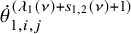 with respect to the loop filtration is
$\theta _{1,i,j; \lambda _1(\nu ) + s_{1,2}(\nu )}$
 .
Using Lemma 5.5(2)(ii) and (iii) we see that the associated graded with respect to the loop filtration
$\operatorname {gr}(R(^\nu y_n(\sigma ), \tau )/I)$
 is generated as a commutative algebra by the top filtered component of the elements (6.5) modulo (5.76). The proof now proceeds as in case (i).
Remark 6.3. This paper was built upon the developments made in [Reference TopleyTo23, Part I]. When writing this work we noticed several minor typos in that paper and we list them here for completeness.
-
(1) There is a sign error in [Reference TopleyTo23, (3.29), (3.31)].
-
(2) In [Reference TopleyTo23, (3.70)] $\varpi _{r,s}$
should be replaced with
$\varpi _{s,r}$
-
(3) Definition 3.22 makes no sense the way it is written; the $f_{i,j}$
are defined for
$j> i$
, however the recurrence [Reference Brundan and KleshchevBK06, (2.19)] should be followed. -
(4) The proof of [Reference TopleyTo23, Lemma 4.2] has a double sign error, but these cancel and the stated result is correct.
-
(5) The map in [Reference TopleyTo23, (4.18)] should read $c_{i,i}^{(r - 1)} \mapsto (-1)^{r-1} t^{(r)}_{i,i,i-1}$
.



Acknowledgements
Both authors would like to thank Jon Brown, Jon Brundan, Kang Lu, Hiraku Nakajima, Yung-Ning Peng, Thomas Tappeiner, Weiqiang Wang and Matt Westaway for useful conversations during the development of this work. The first author is grateful to the University of Bath for funding his PhD studies. The second author would like to acknowledge funding from the UKRI Future Leaders Fellowship, grant numbers MR/S032657/1, MR/S032657/2, MR/S032657/3.
Competing interests
The authors have no competing interests to disclose.

 Open access

