

1 Introduction
Multilayer dielectric gratings (MLDGs)[ Reference Svakhin, Sychugov, Tikhomirov, Mason and Anderson 1 – Reference Perry, Boyd, Britten, Decker, Shore, Shannon and Shults 3 ] are key components in high-power laser systems[ Reference Strickland and Mourou 4 – Reference Treacy 6 ] to exhibit both high diffraction efficiency (DE) to ensure spectral performance[ Reference Wang, Jin, Ma, Shao and Fan 7 – Reference Park, Oh, Moon and Cho 12 ] and strong damage resistance to withstand laser-induced damage[ Reference Bonod and Neauport 13 ]. Dielectric materials exhibit higher laser-induced damage thresholds (LIDTs) than metals due to their low extinction coefficients[ Reference Perry, Stuart, Banks, Feit, Yanovsky and Rubenchik 14 – Reference Rodríguez-de Marcos, Larruquert, Méndez and Aznárez 17 ]. However, when achieving high efficiency, the resonant sub-wavelength structure still results in the enhancement of the localized electric-field intensity (EFI) within the gratings[ Reference Neauport, Lavastre, Razé, Dupuy, Bonod, Balas, De Villele, Flamand, Kaladgew and Desserouer 18 ]. This EFI enhancement constrains the LIDT, limiting its use in modern laser systems that demand higher power.
Extensive research has been dedicated to suppressing EFI within MLDGs for specific applications. Liu et al. [ Reference Liu, Shen, Kong, Shen, Deng, Zhao, Shao and Fan 19 ] found that a rectangular grating, larger angle of incidence (AOI) and higher refractive index material could reduce the gratings’ EFI. Guan et al. [ Reference Guan, Jin, Liu, Kong, Du, He, Yi and Shao 20 ] and Diop et al. [ Reference Diop, Bonod, Chorel, Lavastre, Roquin, Heymans, Brianceau, Gallais and Lamaignère 21 ] observed that certain variations in the thickness and refractive index of the matching layer can simultaneously increase DE and decrease EFI. However, optimizing individual parameters is insufficient for determining the full set of grating parameters, particularly when certain constraints exist (e.g., fixed AOI or grating material). Theoretical approaches, such as the modal analysis for binary dielectric transmission gratings proposed by Clausnitzer et al. [ Reference Clausnitzer, Kaempfe, Kley, Tuennermann, Tishchenko and Parriaux 22 , Reference Clausnitzer, Kämpfe, Kley, Tünnermann, Peschel, Tishchenko and Parriaux 23 ], successfully deduced conditions for high DE using a simple transmission phase formula, but the method was inapplicable to EFI calculation. As a result, improving LIDT while maintaining high DE remains to be accomplished by numerical optimization. Strategies that combine merit functions with genetic algorithms[ Reference Guan, Jin, Liu, Kong, Du, He, Fang, Yi and Shao 24 – Reference Sun, Li, Chen, Xu, Sun and Lin 26 ], simulated annealing algorithm[ Reference Hu, Zhou, Wu, Yu, Cao and Jia 27 ] or particle swarm optimization[ Reference Xie, Zhang, Zhang, Ma, Li, Wang and Cheng 28 ] are the most commonly applied approaches to co-optimize DE and EFI. Despite their flexibility in defining optimization targets, these merit-function-based approaches are limited to predefined parameter ranges, provide minimal physical explanation and lack a global optimization strategy. These limitations make it difficult to compare optimization results across methods, and offer little practical guidance for selecting suitable structures when material choices and fabrication constraints should be considered.
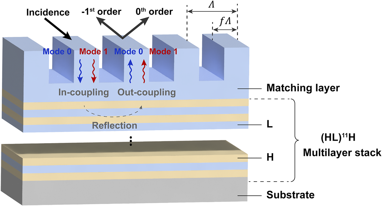
Schematic of the MLDG structure. The duty cycle
$f$
 is defined as the ratio of the ridge width
$f\varLambda$
 to the grating period
$\varLambda$
 . Two Bloch modes (modes 0 and 1) propagate through the grating layer and are reflected by the multilayer structure; the modes out-couple into free space as 0th and –1st diffraction orders.

Figure 1 Long description
The diagram illustrates the M L D G structure starting from the top surface.
* At the top, an arrow labeled Incidence points to a blue rectangular ridge. Above the ridges, two arrows point away from the surface representing the minus 1st order and 0th order diffraction.
* The grating geometry is defined by a period Lambda and a ridge width f Lambda.
* Within the blue grating layer, blue and red wavy arrows represent Mode 0 and Mode 1. These modes move downward during In-coupling and upward during Out-coupling.
* Below the grating is a Matching layer, followed by a Multilayer stack labeled (H L) super 11 H. This stack consists of alternating light yellow layers labeled H and light blue layers labeled L.
* A dashed curved arrow within the stack indicates Reflection.
* The entire assembly sits on a thick grey base labeled Substrate.
Here, we propose a phase-matching design framework for MLDGs based on classic modal analysis and an extended theory of EFI. The framework employs rigorous coupled-wave analysis (RCWA) and the finite element method (FEM) to reliably simulate the variations in DE and EFI, with DE behavior further interpreted through propagation phase theory. The periodic dependencies of DE and EFI on matching layer thickness are systematically examined using an extended interfacial phase analysis. This leads to a phase-matching framework designed to align the DE peak with the EFI valley. The evolution and redistribution of the electric field are calculated and analyzed using the FEM. The framework is first implemented and validated with low-index SiO2, and then tested with high-index HfO2, demonstrating robustness across material systems. This approach provides guidance for designing MLDGs with specific requirements on both efficiency and LIDT.
2 Numerical calculation
To investigate how structural parameters influence the DE and EFI, we calculated the DE and localized peak EFI of a representative MLDG as functions of duty cycle and groove depth. In this work, EFI refers to the localized peak EFI within the structure normalized by the incident field. The FEM was used for the main calculations, and RCWA was employed for cross-validation. The representative structure is shown in Figure 1. In the simulation, all structural parameters except the duty cycle and groove depth were fixed. The substrate was fused silica, and the multilayer stack adopted an (HL)11H quarter-wave design at 1064 nm, where H and L correspond to HfO2 and SiO2 layers, respectively. Both the matching layer and the grating were composed of SiO2, and the matching layer thickness was fixed at 300 nm. The grating period was set to 614 nm to satisfy the Littrow condition[ Reference Delabachelerie and Passedat 29 ]. The incident light was TE-polarized, with a wavelength of 1064 nm and an AOI of 60°. The duty cycle and groove depth were scanned over 0–1 and 0–3000 nm, respectively.
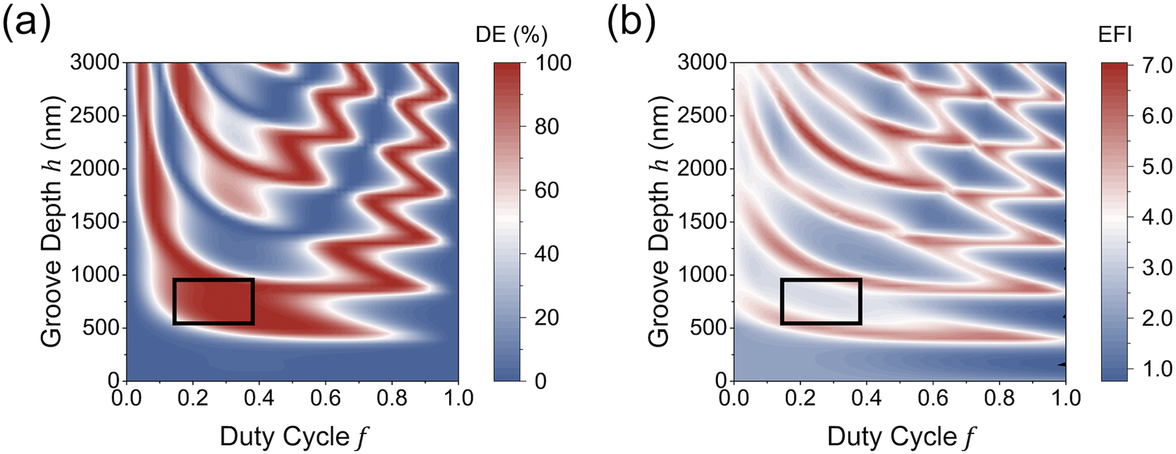
As depicted in Figures 2(a) and 2(b), similar patterns are observed, revealing an inherent limitation between DE and EFI. The black-outlined region in Figure 2 demonstrates that high DE and low EFI can be achieved simultaneously, confirming the feasibility of co-optimization. Moreover, this region corresponds to a broad parameter range (groove depth and duty cycle), which implies a high tolerance to fabrication errors.
(a) The DE and (b) EFI as functions of duty cycle and groove depth by FEM simulations. The fixed parameters are an (HL)11H quarter-wave multilayer stack (with H representing HfO2 and L representing SiO2) at 1064 nm, a SiO2 matching layer (300 nm thick) and a grating with a period of 614 nm (Littrow condition). The substrate is fused silica, and the incident light is TE-polarized at 1064 nm with an AOI of 60°. The black-outlined region denotes the ideal structures featuring high DE and low EFI.

Figure 2 Long description
Two side-by-side heat maps, labeled a and b, share identical axes. The horizontal x-axis represents Duty Cycle f ranging from 0.0 to 1.0. The vertical y-axis represents Groove Depth h in nanometers, ranging from 0 to 3000.
Panel a displays D E percentage. The color scale on the right ranges from blue at 0 to dark red at 100. The plot shows a series of curved, oscillating bands of high D E (red) and low D E (blue) that originate from the left and sweep toward the top-right. A black-outlined rectangular region is located between duty cycles 0.15 and 0.4, and groove depths 550 and 950 nanometers. This region is filled with solid dark red, indicating a D E near 100 percent.
Panel b displays E F I. The color scale on the right ranges from blue at 1.0 to dark red at 7.0. The plot shows similar curved interference patterns, but the intensity distribution is different. In the same black-outlined rectangular region (duty cycle 0.15 to 0.4, groove depth 550 to 950 nanometers), the color is light blue to white, indicating a low E F I value between 1.0 and 2.0.
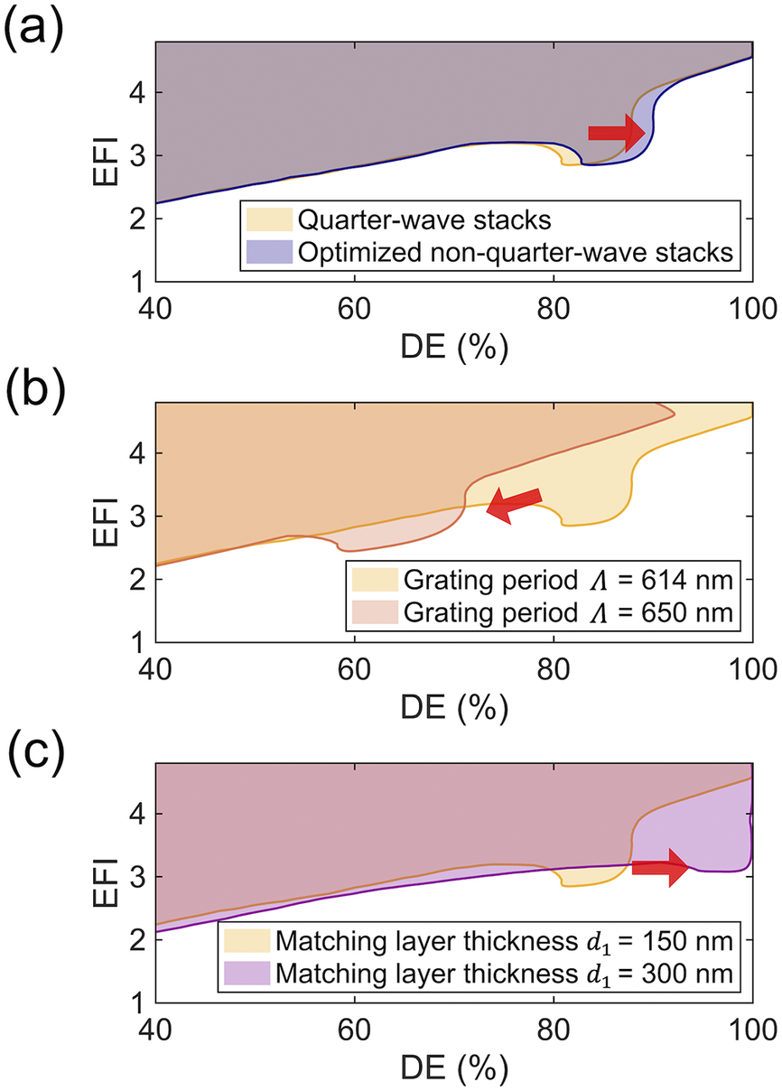
To understand how each parameter affects the balance between DE and EFI, we employ a straightforward parameter-scanning approach. In each case, we scan the grating’s duty cycle (0.2–0.8) and groove depth (0–1200 nm) while modifying only one of the fixed parameters from Figure 2 (multilayer stacks, grating period and matching layer thickness) at a time – keeping all other conditions unchanged. For every structure simulated in such a scan, we obtain a corresponding pair of DE and EFI values. Plotting these pairs with DE as the horizontal coordinate and EFI as the vertical coordinate yields a scattered DE–EFI distribution. These DE–EFI data points occupy certain regions in the plot, which are shown as shaded regions in Figure 3; the lower envelopes of these regions are extracted and smoothed as the boundary curves. The boundary curves extend from the lower left to the upper right, illustrating the inherent DE–EFI trade-off: higher DE generally comes with higher EFI.
DE–EFI trade-off plots for different (a) multilayer stacks, (b) grating periods and (c) matching layer thicknesses. For each case, the duty cycle (0.2–0.8) and groove depth (0–1200 nm) are fully scanned in the same way as in Figure 2, generating a cloud of data points (DE on the horizontal axis, EFI on the vertical axis) that exhibit a boundary. The shift of this boundary indicates how each parameter influences the possibility of achieving both high DE and low EFI. The matching layer thickness is 150 nm. Other structural parameters are fixed as in Figure 2.

Figure 3 Long description
The figure consists of three panels, a, b, and c, each sharing the same axes: the horizontal x-axis represents D E in percent ranging from 40 to 100, and the vertical y-axis represents E F I ranging from 1 to 4.
Panel a compares Quarter-wave stacks in yellow and Optimized non-quarter-wave stacks in purple. Both datasets show a boundary that rises as D E increases. A red arrow points to the right, indicating that optimized stacks shift the boundary toward higher D E values at similar E F I levels.
Panel b compares Grating period Lambda equals 614 nanometers in yellow and Grating period Lambda equals 650 nanometers in orange. A red arrow points to the left, showing that increasing the grating period shifts the performance boundary toward lower D E values.
Panel c compares Matching layer thickness d sub 1 equals 150 nanometers in yellow and Matching layer thickness d sub 1 equals 300 nanometers in purple. A red arrow points to the right, indicating that a thicker matching layer shifts the boundary toward higher D E values, particularly in the 80 to 100 percent range.
Since our goal is to achieve high DE and low EFI, a boundary that shifts toward the bottom-right corner indicates a better chance of finding the optimal solution. Thus, by observing how the boundary moves when a fixed parameter is changed, we can directly evaluate whether that parameter helps improve the performance toward our target.
As shown in Figure 3(a), changing from a standard quarter-wave stack to an optimized non-quarter-wave stack (with each layer thickness individually tuned) shifts the boundary only slightly to the right. This shift indicates a modest increase in DE, which we attribute to the enhanced reflectivity of the optimized stack, while EFI remains almost unchanged. In contrast, deviating the grating period from the Littrow condition (Figure 3(b)) forces the boundary to contract sharply toward the lower left, confirming that the period is not a viable degree of freedom for co-optimization. Most notably, adjusting the matching layer thickness (Figure 3(c)) produces a clear expansion of the boundary toward the desired bottom-right corner, identifying this parameter as a promising lever for co-optimization. Detailed analyses of these behaviors are provided in the following sections.
3 Propagation phase analysis for diffraction efficiency
The parameter scan presented in Figure 2(b) revealed that achieving high DE requires the grating period to satisfy the Littrow condition. To understand this behavior theoretically, we apply the modal analysis established by Clausnitzer et al.
[
Reference Clausnitzer, Kämpfe, Kley, Tünnermann, Peschel, Tishchenko and Parriaux
23
]. The modal analysis is conducted under the Littrow condition, under which multiple modes vanished to Bloch modes 0 and 1 with the effective refractive indices of
${n}_{\mathrm{eff1}}$
 and
${n}_{\mathrm{eff2}}$
 , respectively. Deviating from the Littrow condition – such as altering the grating period – reduces DE. The DE of 0th and –1st diffraction orders is determined by the phase difference
$\Delta \varphi$
 of Bloch modes 0 and 1[
Reference Dong, Zhang, Xie, Zhu, Liang, Wei, Shi, Tikhonravov, Wang, Zhou and Cheng
30
,
Reference Lalanne, Hugonin and Chavel
31
]:

Here,
$\Delta {\varphi}_{\mathrm{prop}}$
 denotes the difference between the propagation phases for two Bloch modes, given by
$2{k}_0\Delta {n}_{\mathrm{eff}}h$
 , where
${k}_0$
 is the incident wavevector in free space,
$\Delta {n}_{\mathrm{eff}}$
 is the difference between the effective refractive indices for two Bloch modes, which depends on the duty cycle and grating material, and
$h$
 is the groove depth. The terms
${\Delta \varphi}_{\mathrm{ref}},{\Delta \varphi}_{\mathrm{in}}$
 and
${\Delta \varphi}_{\mathrm{out}}$
 represent the difference between reflection phases, in-coupling phases and out-coupling phases, respectively. Their summation is referred to as the difference of interfacial phases
${\Delta \varphi}_{\mathrm{inter}}$
 , which is small compared to
${\Delta \varphi}_{\mathrm{prop}}$
 [
Reference Dong, Zhang, Xie, Zhu, Liang, Wei, Shi, Tikhonravov, Wang, Zhou and Cheng
30
,
Reference Lalanne, Hugonin and Chavel
31
] and is neglected in theoretical DE calculations. In addition, the –1st order DE can be written as follows:

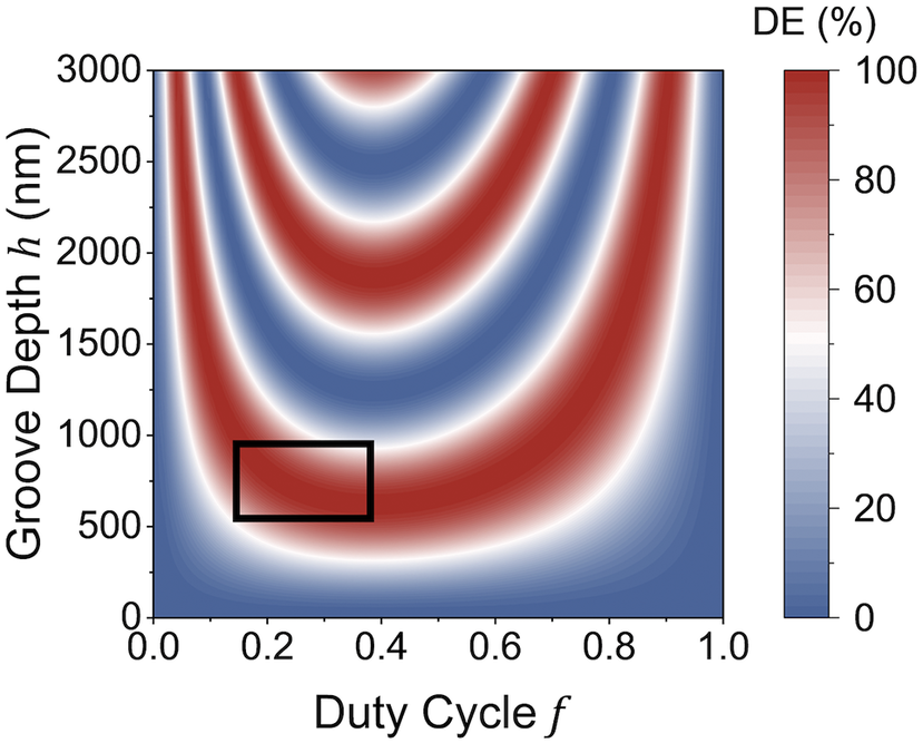
The theoretical DE as a function of duty cycle and groove depth calculated using Equation (2) is displayed in Figure 4, and its overall trend generally aligns with the simulation results in Figure 2(a). Therefore, the high-DE structures can be preliminarily estimated using the Littrow condition and Equation (2), streamlining the subsequent optimization process.
Theoretical DE as a function of the duty cycle and groove depth calculated by Equation (2). All structural parameters are consistent with those used in Figure 2, and the black-outlined region denotes the ideal structures as in Figure 2.

Figure 4 Long description
The X-axis represents Duty Cycle f, ranging from 0.0 to 1.0. The Y-axis represents Groove Depth h in nanometers, ranging from 0 to 3000. A vertical color bar on the right indicates D E percentage, where dark blue represents 0 percent, white represents 50 percent, and dark red represents 100 percent.
Data Trends:
* The plot displays a series of alternating red and blue U-shaped bands that originate from the top edge and curve toward the bottom.
* At low groove depths below 500 nanometers, the D E remains mostly blue (low efficiency) across all duty cycles.
* As groove depth increases, the bands become more frequent and narrower.
* A black-outlined rectangular region is located between duty cycles 0.15 and 0.4, and groove depths 500 and 1000 nanometers. This region encompasses a dark red peak, indicating high D E efficiency for these specific structural parameters.
4 Interfacial phase extension
As discussed in Section 3, when only the grating layer is considered, DE is primarily governed by
${\Delta \varphi}_{\mathrm{prop}}$
 . For the layer region beneath the grating where
${\Delta \varphi}_{\mathrm{prop}}$
 approaches zero, however, the influence of
${\Delta \varphi}_{\mathrm{inter}}$
 on the overall grating performance should be taken into account. We applied the transfer matrix method to understand
${\Delta \varphi}_{\mathrm{inter}}$
 . For each Bloch mode, the transfer matrix of the entire
$p$
 -layer stack (including the matching layer and the multilayer stack) is as follows[
Reference Born and Wolf
32
]:

where
$m=1$
 denotes the matching layer and the phase thickness
${\delta}_m$
 is defined as follows:

and the admittance for TE polarization is as follows:

The equivalent admittance of the entire
$p$
 -layer stack is as follows:

At the interface between the grating layer and the matching layer, the reflection coefficient is as follows:

where
${\eta}_0$
 is the admittance of the grating layer, which takes different values for the two Bloch modes. This difference leads to different reflection coefficients and the resulting
${\Delta \varphi}_{\mathrm{inter}}$
 . It explains why distinct results are obtained when fine-tuning the multilayer stack (Figure 3(a)) versus changing the matching layer thickness (Figure 3(c)). The former only involves subtle, reflectance-oriented adjustments and thus has minimal impact on
${\Delta \varphi}_{\mathrm{inter}}$
 , whereas the latter directly affects
${\Delta \varphi}_{\mathrm{inter}}$
 via admittance. Consequently,
${\Delta \varphi}_{\mathrm{inter}}$
 modulated by the matching layer thickness serves as a key factor for the co-optimization of DE and EFI. To ensure the generality of the results, we adopted the standard quarter-wave multilayer stack (HL)11H in the subsequent calculations.
After appropriate simplification of Equations (3)–(6), the following expression is obtained:

where
${Y}_2$
 is the equivalent admittance of the multilayer stack excluding the matching layer, which is fixed for the given (HL)11H design. Due to the presence of the
$\tan {\delta}_1$
 term,
$Y$
 is a periodic function of
${\delta}_1$
 with a period of
$\pi$
 . Since
${\Delta \varphi}_{\mathrm{inter}}$
 is related to
$Y$
 , both the EFI and the DE, which are modulated by
${\Delta \varphi}_{\mathrm{inter}}$
 , are also periodic functions of
${\delta}_1$
 with a period of
$\pi$
 . According to Equation (4), which relates the phase thickness to the physical thickness, the DE and the EFI are also periodic functions of the matching layer thickness
${d}_1$
 , with the corresponding period
$T$
 given by the following:

where
$\ell$
 is a positive integer. Based on Equation (9), the designed grating features a period of 452.6 nm.
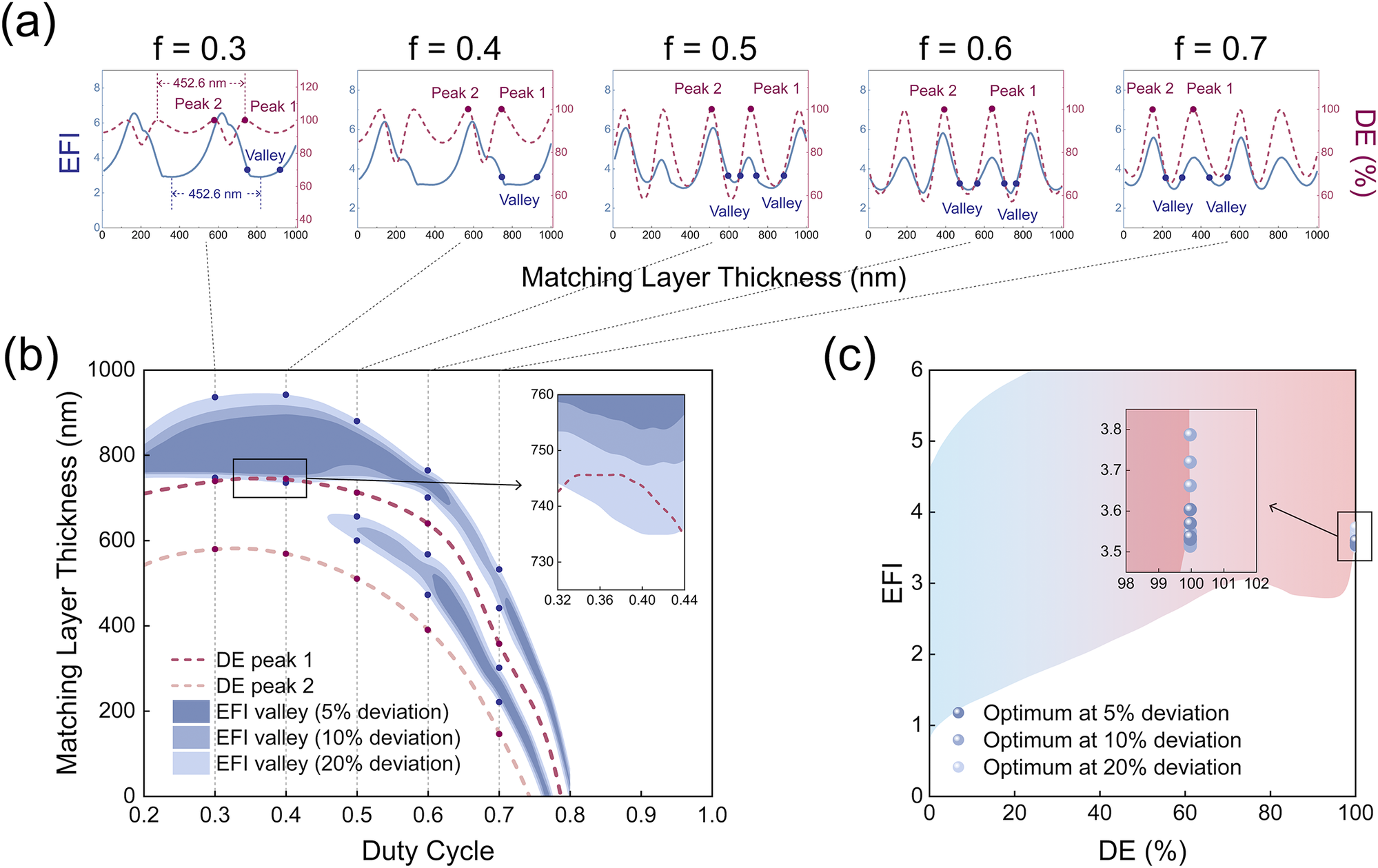
Under various duty cycles, we evaluated the DE and EFI as functions of the matching layer thickness. For each duty cycle, the groove depth was calculated using Equation (2) to maintain the high-DE condition. Selected results for duty cycles of 0.3, 0.4, 0.5, 0.6 and 0.7 are shown in Figure 5(a). The results all exhibit clear periodic behavior, consistent with theoretical predictions. Within each period, there are two DE peaks and one or two EFI valleys. A mismatch exists between the matching layer thicknesses corresponding to the DE peaks and EFI valleys, and its magnitude varies with the duty cycle. Ideally, if this mismatch could be eliminated (i.e., the DE peak aligns with the EFI valley, a condition we term phase-matching), a single matching layer thickness could simultaneously achieve high DE and low EFI in one structure.
Phase-matching strategy for co-optimization of DE and EFI for the SiO2 grating. (a) DE and EFI as functions of matching layer thickness at selected duty cycles (0.3–0.7). (b) Matching layer thicknesses for DE peaks (dashed red lines) and EFI valleys (blue shadowed regions) for duty cycles from 0.2 to 0.8 in steps of 0.01. The EFI valleys are defined with deviations of 5%, 10% and 20%. (c) Global parameter scan results (duty cycle from 0.2 to 0.8, groove depth from 0 to 3000 nm, matching layer thickness across one full period
$T$
 ). The filled blue circles mark the optimal solutions obtained by our method.

Figure 5 Long description
Panel a contains five line graphs for duty cycles f equals 0.3, 0.4, 0.5, 0.6, and 0.7. Each graph plots E F I on the left y-axis (solid blue line) and D E percentage on the right y-axis (dashed red line) against Matching Layer Thickness from 0 to 1000 nanometers. As f increases, the number of E F I valleys and D E peaks increases, with specific points labeled Peak 1, Peak 2, and Valley.
Panel b is a large plot of Matching Layer Thickness (0 to 1000 nanometers) versus Duty Cycle (0.2 to 1.0). It features two dashed red curves for D E peak 1 and D E peak 2. Blue shadowed regions represent E F I valleys at 5 percent, 10 percent, and 20 percent deviation. An inset zooms into the region between duty cycles 0.32 and 0.44. Blue dots mark the intersection of D E peaks and E F I valleys.
Panel c is a scatter plot of E F I (0 to 6) versus D E percentage (0 to 100). A large shaded region transitions from blue on the left to red on the right. An inset at D E equals 100 percent shows optimal solutions as filled blue circles for 5 percent, 10 percent, and 20 percent deviations, clustered between E F I values of 3.5 and 3.8.
To explore this possibility, we systematically varied the duty cycle from 0.2 to 0.8 in steps of 0.01 and recorded the matching layer thicknesses corresponding to each DE peak and EFI valley within the same period. These data are plotted in Figure 5(b). Since the EFI valleys are not sharply defined, especially at lower duty cycles, we introduced a specific deviation into their definition. A valley was considered valid if its EFI value did not exceed the minimum of that curve by more than a given percentage. Deviations of 5%, 10% and 20% were applied (e.g., for a 20% deviation, the valid EFI is ≤120% of the local minimum). For visual clarity, the DE peaks are marked with red dots, and the EFI valley ranges defined by the 20% deviation are marked with blue dots in Figures 5(a) and 5(b). In Figure 5(b), the two DE peaks are represented by red dashed lines, and the EFI valleys for the three deviations are represented by blue shadowed regions of varying intensity. As the deviation increases, the blue shadowed region expands, indicating a greater chance of overlap between a DE peak and an EFI valley. For deviations of 5% and 10%, the points where DE peak 1 is closest to the EFI valley can be regarded as the optimal structures. When the deviation reaches 20%, a small overlap region appears between DE peak 1 and one of the EFI valleys (see the inset in Figure 5(b)). Within this overlap region, the duty cycle ranges from 0.33 to 0.43, and the matching layer thickness ranges from 738 to 746 nm (or 285–293 nm because of the periodicity). In this parameter range, both high DE and low EFI can be achieved simultaneously.
To determine whether the solutions from the overlap region represent the global optima for co-optimizing DE and EFI, we compared them with results from a comprehensive parameter scan. The scan varied three parameters simultaneously: the duty cycle (0.2–0.8), groove depth (0–3000 nm) and matching layer thickness (across one full period
$T$
 ). The results are shown in Figure 5(c), where the data points again form a distinct boundary similar to that in Figure 3. The solutions from the overlap region identified via our phase-matching analysis are marked by filled blue circles. These solutions lie in the lower-right corner of the plot, confirming their status as globally optimal solutions for achieving high DE and low EFI. As the allowed EFI deviation increases, the solutions shift upward slightly. Due to minor fluctuations in the absolute EFI valley values, some circles within higher-deviation regions can still correspond to relatively low EFI, causing them to appear lower in the plot.
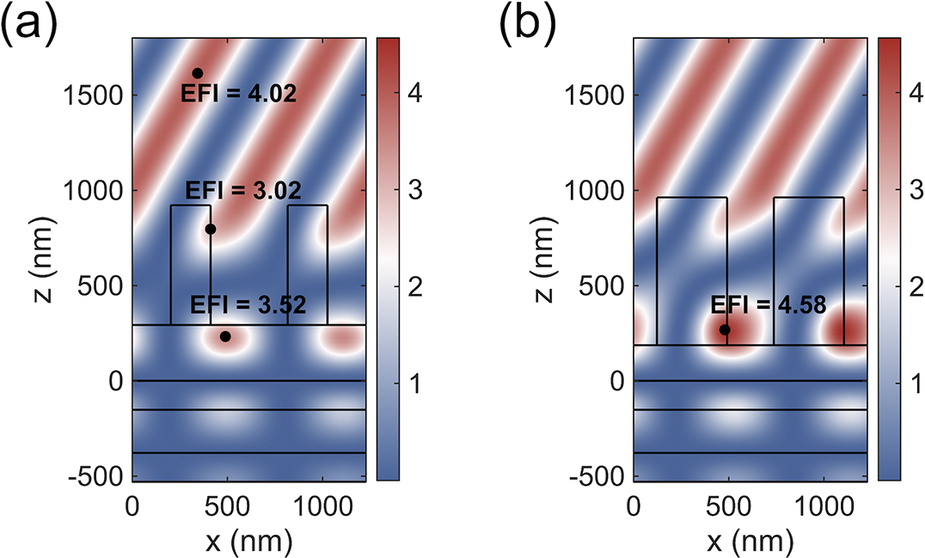
Figure 6 illustrates the differences in the spatial distributions of EFI between two structures identified from our phase-matching analysis: the optimal structure, where the DE peak aligns closely with the EFI valley (with a duty cycle of 0.34, a groove depth of 629.0 nm and a matching layer thickness of 293 nm), and the worst structure, where the DE peak is most misaligned with the EFI valley (with a duty cycle of 0.6, a groove depth of 775.6 nm and a matching layer thickness of 187 nm). In the optimal structure shown in Figure 6(a), the region of strongest EFI is effectively guided into the air region above the grating ridges, thereby reducing EFI inside the structure and improving laser resistance. By contrast, in Figure 6(b), the highest EFI occurs inside the grating ridges. This clear distinction confirms that the phase-matching strategy relocates the EFI peak from the grating material into the adjacent air space, ensuring low EFI without compromising high DE.
The EFI distributions for two grating structures. (a) The optimal structure with the DE peak aligned to the EFI valley. (b) The opposite structure with the DE peak aligned to the EFI peak. Black points denote the peak EFI in the full MLDG, on the grating pillars and across the entire domain, and in (b), they coincide at a single location.

Figure 6 Long description
Two heat maps, labeled a and b, plot z in nanometers on the vertical axis from negative 500 to 1500 against x in nanometers on the horizontal axis from 0 to 1200. A color scale on the right of each panel ranges from 1 in blue to over 4 in red. Both panels show a layered substrate below z equals 0 and rectangular grating pillars above.
In panel a, the E F I distribution shows diagonal bands of alternating intensity. Three black dots mark specific points. The highest dot at z equals 1600 is labeled E F I equals 4.02. A dot on the edge of a pillar is labeled E F I equals 3.02. A dot in the substrate valley is labeled E F I equals 3.52.
In panel b, the E F I peaks are concentrated at the base of the grating pillars. A single black dot is placed at the center of a high-intensity red peak at the base of a pillar, labeled E F I equals 4.58. This single point represents the peak E F I for the full M L D G, the pillars, and the entire domain simultaneously.
Having validated the phase-matching strategy using the common low-refractive-index material SiO2, we further tested its robustness by replacing the grating material with HfO2, a standard high-refractive-index material for high-power applications, while keeping the multilayer stack and grating period unchanged. The groove depth for each duty cycle was adjusted accordingly using Equation (2).
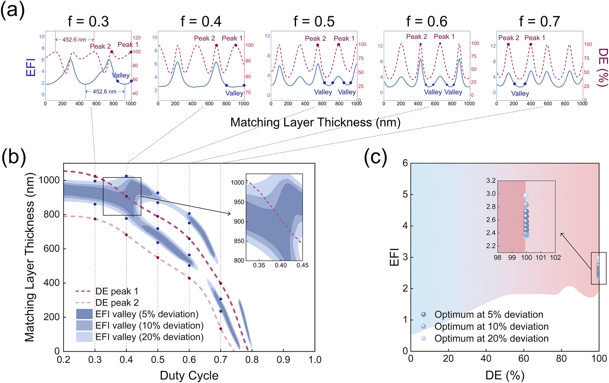
Figure 7(a) shows how DE and EFI vary with matching layer thickness at duty cycles of 0.3, 0.4, 0.5, 0.6 and 0.7, respectively. Similarly, the results maintain a consistent periodicity, with two DE peaks and one or two EFI valleys within each period. As with SiO2, a mismatch exists between the matching layer thicknesses for DE peaks and EFI valleys. We performed the same systematic analysis as before, varying the duty cycle from 0.2 to 0.8 in steps of 0.01. Figure 7(b) plots the positions of DE peaks and EFI valleys, with the latter defined using the same deviations (5%, 10% and 20%). The overlap region between DE peak 1 and the EFI valley is larger compared to the case with SiO2, and the overlap occurs across all three deviations. The inset shows that at the 20% deviation, the overlap region corresponds to a duty cycle range of 0.34–0.44 and a matching layer thickness range of 854–988 nm (or 401–535 nm because of the periodicity).
Phase-matching strategy for co-optimization of DE and EFI for the HfO2 grating. (a) DE and EFI as functions of matching layer thickness at selected duty cycles (0.3–0.7). (b) Matching layer thicknesses for DE peaks (dashed red lines) and EFI valleys (blue shadowed regions) for duty cycles from 0.2 to 0.8 in steps of 0.01. The EFI valleys are defined with deviations of 5%, 10% and 20%. (c) Global parameter scan results (duty cycle from 0.2 to 0.8, groove depth from 0 to 3000 nm, matching layer thickness across one full period
$T$
 ). The filled blue circles mark the optimal solutions obtained by our method.

Figure 7 Long description
Panel a contains five line graphs for duty cycles f equals 0.3, 0.4, 0.5, 0.6, and 0.7. The x-axis is Matching Layer Thickness in nanometers from 0 to 1000. The left y-axis is E F I in blue and the right y-axis is D E percent in purple. D E is shown as a dashed purple line with periodic peaks labeled Peak 1 and Peak 2. E F I is a solid blue line with periodic valleys. As f increases, the D E peaks shift and the E F I valleys become more pronounced.
Panel b is a large plot of Matching Layer Thickness from 0 to 1000 nanometers versus Duty Cycle from 0.2 to 1.0. Two dashed red lines track the positions of D E peak 1 and D E peak 2, both showing a downward curve as duty cycle increases. Blue shadowed regions represent E F I valleys at 5 percent, 10 percent, and 20 percent deviation. An inset zooms into the region where the D E peak 1 line intersects the E F I valley contours between duty cycles 0.35 and 0.45.
Panel c is a scatter plot of E F I from 0 to 6 versus D E percent from 0 to 100. The background is a gradient from blue on the left to red on the right. Optimal solutions are marked with blue circles concentrated at 100 percent D E. An inset shows a vertical stack of these points at exactly 100 percent D E with E F I values ranging between 2.2 and 3.0, categorized by 5 percent, 10 percent, and 20 percent deviation levels.
A full parameter scan (Figure 7(c)) confirms that these solutions from the overlap region (marked by filled blue circles) occupy the global optimal region in the DE–EFI co-optimization space. This demonstrates the method’s robustness and general applicability across different material systems.
The consistency between the SiO2 and HfO2 grating results supports the robustness of the proposed phase-matching strategy. Furthermore, the method provides a structured framework for material selection under specific performance targets. The optimal parameter ranges identified – duty cycles of 0.33–0.43 with matching layer thicknesses of 738–746 or 285–293 nm for SiO2, and duty cycles of 0.34–0.44 with thicknesses of 854–988 or 401–535 nm for HfO2 – reveal the inherent fabrication tolerance associated with each material system. By comparing these tolerance ranges with standard process capabilities, this approach can help assess whether a given material can be reliably manufactured under practical constraints. For example, in cases where material choice is flexible, HfO2 may be advantageous due to its broader tolerance, which can accommodate common process variations such as the ±5% linewidth uniformity in reactive ion etching and the ±2% thickness uniformity in magnetron sputtering. Conversely, if the application requires a low-index material such as SiO2, the method clarifies the necessary precision – such as thickness control within approximately 9 nm – which should be achieved using specific techniques. Thus, the strategy not only aids in co-optimizing DE and EFI but also helps translate optical performance targets into practical fabrication considerations, offering a useful connection between design intent and manufacturability to support more informed material and process decisions.
Notably, when practical applications demand stricter EFI suppression and allow some compromise in DE, the method can be symmetrically extended by also introducing a permitted deviation for the DE peak – for instance, allowing the selected DE value to be a certain percentage lower than its local maximum. In such cases, the resulting optimal solutions will trace along the EFI–DE boundary curve toward the lower-left region in Figures 5(c) and 7(c).
This optimization strategy advances beyond purely data-driven approaches by clarifying the theoretical bounds of the EFI–DE relationship, identifying practical global optima and facilitating efficient design. Crucially, it reveals the general variation patterns of DE and EFI with respect to key parameters, marking a significant step from empirical observation toward theoretical understanding. However, certain deeper physical mechanisms – particularly the spatial distribution of the localized electric field within the grating structure – remain to be fully resolved. Future studies will investigate these electromagnetic patterns to establish a predictive model linking near-field behavior to overall grating performance. Furthermore, with DE exceeding 99.9%, the high-refractive-index material exhibits a lower EFI, revealing a general inverse relationship between refractive index and EFI under high-DE conditions. Practical issues, including material intrinsic properties[ Reference Wen, Zhu, Chai, Liu, Shi, Du and Shao 33 ] and fabrication constraints[ Reference Sridharan, Pramitha and Bhattacharya 34 ], are also important factors to be considered in further research.
5 Conclusion
In this study, we proposed a phase-matching strategy for the co-optimization of DE and EFI in MLDGs. We first applied propagation phase analysis based on the modal method to identify high-DE structures, which provided the duty cycle and groove depth combinations that satisfy the Littrow condition. Using the transfer matrix method, we then introduced the interfacial phase arising from reflections at the grating–matching layer interface. This analysis revealed that both DE and EFI exhibit a periodic dependence on the matching layer thickness, with the period analytically determined to be 452.6 nm – consistent with our theoretical analysis. By examining how the positions of DE peaks and EFI valleys vary with duty cycle, we established a design criterion that aligns the DE peak with the EFI valley – termed phase-matching. Applying this criterion, we identified globally optimal structures that achieve DE exceeding 99.9% while minimizing EFI, with the peak electric field relocated from the interior of the grating ridges to the air interface above them. This work provides a physics-based framework that moves beyond purely numerical optimization toward a predictive, principle-guided approach to MLDG design.
One of the key outcomes of our strategy is the identification of well-defined and manufacturable parameter regions, which directly translate into practical fabrication tolerances for critical parameters such as duty cycle and matching layer thickness. This ensures robust performance under typical process variations. The effectiveness and generality of the approach are further validated through its consistent success across two distinct grating materials: SiO2 and HfO2, representing typical low- and high-refractive-index materials, respectively. This broad validation indicates that the proposed framework is not material-specific and can be reliably extended to other dielectric materials and potentially across a spectral range from the visible to near-infrared. Moreover, the framework is versatile and can be adapted to meet specific DE and EFI requirements, offering flexibility for diverse application scenarios.
Our work advances the understanding of EFI distribution in grating structures and provides a comprehensive, physics-based methodology for engineering a new generation of high-performance MLDGs with fundamentally enhanced LIDTs, moving from iterative optimization toward physically guided design.
Acknowledgements
The authors express their appreciation to Prof. Igor V. Kozhevnikov for fruitful discussions. This work was supported by the National Natural Science Foundation of China (Grants Nos. 62192772, 62475193, 62305251 and 62192770).





 Open access

