


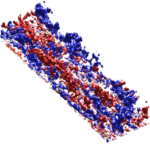



1. Introduction
The interactions of wall-bounded turbulence, between multiple scales and between inner- and outer-region turbulence, are of great scientific interest, as they become increasingly complex with increasing Reynolds numbers. A classical view of wall-bounded turbulence is that the generation of small-scale or large-scale turbulence is due to self-sustained mechanisms (e.g. Hamilton, Kim & Waleffe Reference Hamilton, Kim and Waleffe1995; Jiménez & Pinelli Reference Jiménez and Pinelli1999; Panton Reference Panton2001; Schoppa & Hussain Reference Schoppa and Hussain2002; Hwang & Cossu Reference Hwang and Cossu2010, among others). There is also reported evidence of multiscale and inner–outer turbulence interactions in the literature (e.g. Bandyopadhyay & Hussain Reference Bandyopadhyay and Hussain1984; Hunt & Morrison Reference Hunt and Morrison2000; Abe, Kawamura & Choi Reference Abe, Kawamura and Choi2004; Hoyas & Jiménez Reference Hoyas and Jiménez2006; Pirozzoli, Bernardini & Orlandi Reference Pirozzoli, Bernardini and Orlandi2011) and mechanisms that relate to inner–outer interactions, for instance, large-scale modulations (Hutchins & Marusic Reference Hutchins and Marusic2007b; Mathis, Hutchins & Marusic Reference Mathis, Hutchins and Marusic2009; Ganapathisubramani et al. Reference Ganapathisubramani, Hutchins, Monty, Chung and Marusic2012) and cosupporting mechanisms (Toh & Itano Reference Toh and Itano2005). From a mathematical perspective, for instance, the scale-energy balance (Marati, Casciola & Piva Reference Marati, Casciola and Piva2004; Cimarelli, De Angelis & Casciola Reference Cimarelli, De Angelis and Casciola2013; Cimarelli et al. Reference Cimarelli, De Angelis, Jiménez and Casciola2016) and the spectral Reynolds stress equation (Mizuno Reference Mizuno2016; Cho, Hwang & Choi Reference Cho, Hwang and Choi2018; Lee & Moser Reference Lee and Moser2019) provide statistical evidence that the small scales contribute to the large-scale motions and the existence of inverse energy cascades in channels, i.e. opposite from the classical view of the Richardson–Kolmogorov energy cascade.
Recently, Kawata & Alfredsson (Reference Kawata and Alfredsson2018) proposed an interscale transport equation using scale decomposition on the Reynolds stress transport equation for plane Couette flow and they reported the small-scale dependence of Reynolds shear stress for large-scale structures. The present work is motivated by this recent development. Here we investigate the interscale transport equation for a relatively high Reynolds number turbulent boundary layer (TBL). The aim of the present work is to provide fundamental analysis for interscale and spatial transport in TBLs at moderately high Reynolds numbers.
Perhaps the most important question is how this interscale transport mechanism of Reynolds shear stress relates to the interactions between coherent structures in wall-bounded turbulence, such as the hairpin-vortex signatures and low-momentum zones of hairpin packets (e.g. Adrian, Meinhart & Tomkins Reference Adrian, Meinhart and Tomkins2000; Tomkins & Adrian Reference Tomkins and Adrian2003), the vortex clusters (del Álamo et al. Reference del Álamo, Jiménez, Zandonade and Moser2006) and the sweep-ejection pairs (Lozano-Durán, Flores & Jiménez Reference Lozano-Durán, Flores and Jiménez2012). The hairpin-packet paradigm has been widely investigated experimentally (e.g. Head & Bandyopadhyay Reference Head and Bandyopadhyay1981; Adrian et al. Reference Adrian, Meinhart and Tomkins2000; Ganapathisubramani, Longmire & Marusic Reference Ganapathisubramani, Longmire and Marusic2003; Tomkins & Adrian Reference Tomkins and Adrian2003) and numerically using direct numerical simulations (DNS) with significant evidence of hairpins in TBLs (e.g. Wu & Moin Reference Wu and Moin2009). The vortex clusters give an alternative explanation to the aforementioned hairpin-packet paradigm (del Álamo et al. Reference del Álamo, Jiménez, Zandonade and Moser2006), in which negative quadrant events are defined in terms of the second and fourth quadrants of plane of the streamwise and wall-normal velocity fluctuations as ejections ( ${Q2}$) and sweeps (
 ${Q4}$) (Wallace, Eckelmann & Brodkey Reference Wallace, Eckelmann and Brodkey1972; Willmarth & Lu Reference Willmarth and Lu1972). Extensions of work based on this model by Lozano-Durán & Jiménez (Reference Lozano-Durán and Jiménez2014) studied the temporal evolution of three-dimensional structures of Reynolds shear stress in turbulent channels up to friction Reynolds number
 $Re_\tau \approx 4200$ (where
 $Re_\tau$ is the Reynolds number based on the friction velocity
 $u_\tau = \sqrt {\tau _w/\rho }$,
 $\tau _w$ is the wall shear stress and
 $\rho$ is the density, the boundary layer thickness
 $\delta$ and the kinematic viscosity
 $\nu$) and showed that during the lifetimes of these structures, the ejections are generated by shear near the wall and rise to their mean wall-normal distance by vertical advection
 $(+u_\tau )$ before disappearing, whilst sweeps are produced away from the wall and move towards the wall quickly
 $(-u_\tau )$ and they assemble into side-by-side sweep-ejection pairs (Lozano-Durán et al. Reference Lozano-Durán, Flores and Jiménez2012). Lozano-Durán & Jiménez (Reference Lozano-Durán and Jiménez2014) investigated the interactions associated with tall-attached sweep and ejection events. They found that the merging and splitting of large-scale sweeps and ejections with small-scale structures are prevalent processes during their lifecycle and those interactions are well-balanced over a broad range of scales.
In addition to the channels, Fiscaletti, de Kat & Ganapathisubramani (Reference Fiscaletti, de Kat and Ganapathisubramani2018) studied the intense quadrant events in TBLs. They revealed that quadrant events in TBLs have smaller vertical convection velocities when compared with channel flows, and the intense ejection events are smaller than the intense sweep events, which is likely due to the presence of entrainment. In both models, ejections and sweeps are important constituents in the ensemble-averaged point of view, also because of their well known substantial contribution to the Reynolds shear stress and they are expected to be broadband length scale structures. Therefore, it is expected that a scale decomposition approach applied to the Reynolds shear stress transport equation will yield in-depth insights into their multiscale characteristics.
Large- and small-scale decomposition performed using spectral filters has been widely utilised for characterising large- and small-scale motions and their interactions. Hutchins & Marusic (Reference Hutchins and Marusic2007b) studied the interactions between large- and small-scale motions in TBLs. By spectral filtering the streamwise velocity fluctuation into large- and small-scale components, they revealed the large-scale modulation on the near-wall scales. A follow up study by Mathis et al. (Reference Mathis, Hutchins and Marusic2009) investigated the Hilbert transform of the decomposed small-scale fluctuation, where the modulation effects were analysed to be the large-scale envelope obtained by Hilbert transformation of the small-scale fluctuation. The study revealed a strong correlation between the near-wall cycle and the large-scale motions associated with the logarithmic region. Subsequently, Ganapathisubramani et al. (Reference Ganapathisubramani, Hutchins, Monty, Chung and Marusic2012) extended the analysis to the frequency domain. They used time series data, obtained by hot-film shear stress sensors with traversing hot-wire probes, and investigated the temporal modulation of the large-scale structures on the smaller scales. By a time scale decomposition with time scales of the order of O( $\delta /U_\infty$), that study revealed the strong wall-normal dependence of the frequency modulation. More recently, Lee & Moser (Reference Lee and Moser2019) examined the large- and small-scale contributions to turbulent kinetic energy and the kinetic energy transport equation using a spectral filter. They examined the streamwise scale decomposition of turbulent kinetic energy production and provided statistical evidence of the interactions between the near-wall and outer turbulence as the large-scale modulation of the near-wall turbulence. In the present study, we examine turbulent kinetic energy and Reynolds shear stress transport by extending the approach of Kawata & Alfredsson (Reference Kawata and Alfredsson2018) to data obtained in a new DNS TBL. The goal of this paper, firstly, is to investigate the interscale transport mechanisms in TBLs and compare them with previous plane Couette flow studies. Secondly, we attempt to understand the relationship between the observed inverse Reynolds shear stress transport and the coherent structures that are responsible for momentum transport, i.e. the ejection and sweep events in TBLs. To this end, the large- and small-scale quadrant events and their contributions to the Reynolds shear stress are analysed statistically using a spectral filter.
The remainder of this paper is organised as follows. In § 2 we first introduce the numerical code and validate the new DNS TBL. In § 3 we extend and summarise the generalised interscale transport equation for TBLs and the alternative forms of scale and spatial fluxes in the turbulent kinetic energy and Reynolds shear stress balance. In § 4 we analyse and discuss the roles of the fluxes. We also identify the major differences and similarities between TBLs and the previous work by Kawata & Alfredsson (Reference Kawata and Alfredsson2018) for plane Couette flow. Finally, in § 5 the length and time scales associated with the Reynolds shear stress transport are investigated and discussed.
2. Numerical procedure
The mean and fluctuating velocity components in the streamwise  $(x)$, wall-normal
 $(y)$ and spanwise
 $(z)$ directions are denoted
 $U$,
 $V$,
 $W$,
 $u$,
 $v$ and
 $w$, respectively. The mean and fluctuating pressure are denoted as
 $P$ and
 $p$, respectively. The operator
 $\langle \cdot \rangle$ indicates spanwise and temporal averages. A superscript
 $(+)$ indicates inner-scaling with kinematic viscosity
 $\nu$ and friction velocity
 $u_\tau$. In addition, the outer scales are the free stream velocity
 $U_\infty$ and boundary layer thickness
 $\delta$ (
 $99\,\%$).
Direct numerical simulations of a TBL up to  ${Re}_\tau = \delta ^{+} \simeq 2020$ or equivalently up to
 ${Re}_\theta = {U_\infty \theta }/\nu \simeq 6700$ (where
 $\theta$ is the momentum thickness) were performed. The DNS solver is based on the fully spectral numerical method, as used by Schlatter & Örlü (Reference Schlatter and Örlü2010), with two-dimensional parallelisation (Li, Schlatter & Henningson Reference Li, Schlatter and Henningson2008). Periodic Fourier series with 3/2 zero-padding full dealiasing are used in the wall-parallel direction and Chebyshev polynomials in the wall-normal direction. A low-amplitude volume force trip is applied to the Navier–Stokes equations at the region very close to the inlet to trigger a rapid transition to turbulent flow. For further details on the method of numerical tripping, the reader is referred to Schlatter & Örlü (Reference Schlatter and Örlü2012). To retain the periodic boundary conditions in the streamwise direction, a fringe region is employed at the downstream of the flow, close to the end of the computational domain. In the fringe region, the flow is damped via a volume force until it returns to the inflow condition (Chevalier, Lundbladh & Henningson Reference Chevalier, Lundbladh and Henningson2007). A total of
 $12\,800 \times 769 \times 1024$ spectral modes are employed. The domain size is
 $x_L \times y_L \times z_L = 10\,000 \times 300 \times 360$ in units of displacement thickness at the inlet of the domain,
 $\delta _0^{*}$. This yields a resolution of
 ${\rm \Delta} x^{+} \simeq 8.6$ and
 ${\rm \Delta} z^{+} \simeq 3.9$. There are at least
 $22$ Chebyshev collocation points within the region
 $y^{+} \simeq 10$. The first grid point away from the wall is at
 $y^{+} \simeq 0.02$ and the maximum spacing is
 ${\rm \Delta} y_{{max}}^{+} \simeq 10$. The time advancement is carried out by a second-order Crank–Nicolson scheme for the viscous terms and a third-order four-stage Runge–Kutta scheme for the nonlinear terms.
2.1. Validation of the DNS boundary layer
Figure 1 shows the inner-scaling mean velocity profile, turbulent intensities, Reynolds shear stress and the  $k$-budget (where
 $k = \langle u_i u_i \rangle /2$ is turbulent kinetic energy) for
 ${Re}_\tau \simeq 2020$. The data is compared and validated against the DNS of the TBL from Sillero et al. (Reference Sillero, Jiménez and Moser2013) at
 ${Re}_\tau \simeq 1998$, showing very good agreement. The one-dimensional spanwise premultiplied velocity spectra are plotted in figure 2 for
 ${Re}_\tau \simeq 2020$. Overall, the figure is consistent with the consensus in the literature: (i) the inner peak at
 ${\lambda _z}^{+} \simeq 100$,
 $y^{+} \simeq 15$ characterises the near-wall structures (Kline et al. Reference Kline, Reynolds, Schraub and Runstadler1967; Smith & Metzler Reference Smith and Metzler1983; Tomkins & Adrian Reference Tomkins and Adrian2003); (ii) the outer peak at
 ${\lambda _z} \simeq 0.7\delta , y \simeq 0.15\delta$ characterises the very large-scale motions (Kim & Adrian Reference Kim and Adrian1999; Tomkins & Adrian Reference Tomkins and Adrian2005; Guala, Hommema & Adrian Reference Guala, Hommema and Adrian2006; Hutchins & Marusic Reference Hutchins and Marusic2007a; Monty et al. Reference Monty, Hutchins, NG, Marusic and Chong2009); (iii) the two peaks in the premultiplied (either
 $k_x$ or
 $k_z$)
 $E_{uu}$ and
 $E_{-uv}$ spectra correspond to the small-scale and large-scale structures that contain the streamwise turbulent kinetic energy and Reynolds shear stress, which are not observed in the
 $E_{vv}$ and
 $E_{ww}$ spectra (Lee & Moser Reference Lee and Moser2015); (iv) the penetration (through the dashed-line linear ridge
 $\lambda _z = 8y$) of the large-scale contribution onto the near-wall region in the
 $E_{uu}$ and
 $E_{ww}$ but are not observed in
 $E_{vv}$ and
 $E_{-uv}$ owing to the impermeability of the wall (Hutchins & Marusic Reference Hutchins and Marusic2007a; Lee & Moser Reference Lee and Moser2015; Hwang Reference Hwang2016).
The inner-scaling of  $(a)$ mean velocity
 $U^{+}$,
 $(b)$ turbulence intensities
 ${{\langle ({u_i u_i})^{1/2} \rangle }^{+}}$ and Reynolds shear stress
 ${\langle uv \rangle }^{+}$, (c)
 $k$-balance
 ${\textrm {D} k^{+}}/{\textrm {D} t}=0$. Symbol (
 $\circ$) for present DNS TBL at
 ${Re}_\tau \simeq 2020$; (– – –) Sillero, Jiménez & Moser (Reference Sillero, Jiménez and Moser2013) at
 ${Re}_\tau \simeq 1998$.

The one-dimensional premultiplied spectra at  ${Re}_\tau \simeq 2020$: (a)
 $k_z E_{uu}^{+}$; (b)
 $k_z E_{vv}^{+}$; (c)
 $k_z E_{ww}^{+}$; (d)
 $k_z E_{-uv}^{+}$. Symbol
 $(\times )$ marks the near-wall streaks at
 $y^{+} \simeq 15$ with average characteristic length scale
 $\lambda _z^{+} \simeq 100$ and the large-scale structures at
 $y \simeq 0.15 \,\delta$ with
 $\lambda _z \simeq 0.7 \,\delta$.

3. Mathematical approach
3.1. Interscale transport equations for boundary layers
An analytical approach for large-scale and small-scale interactions, based on the spectral analysis, was proposed by Kawata & Alfredsson (Reference Kawata and Alfredsson2018) for plane Couette flow. Here, we adopt the approach and extend it to TBLs with zero pressure gradient, as described here. A scale decomposition based on the spanwise Fourier mode and a cutoff length scale  $\lambda _z = 2{\rm \pi} /k_z$ is used to separate the velocity fluctuation into large-scale
 $(u'_i)$ and small-scale components
 $(u''_i)$:
 \begin{equation} {u_i}(\boldsymbol{x},t) = u_i'(k_z,\boldsymbol{x},t)+u_i''(k_z,\boldsymbol{x},t).\end{equation}
The large-scale and small-scale components satisfy
 \begin{equation} \langle u_{i}u_{j} \rangle(y) = \langle u_{i}'u_{j}' \rangle (k_z,y)+ \langle u_{i}''u_{j}'' \rangle(k_z,y).\end{equation}
The governing equations are the incompressible Navier–Stokes equations
 \begin{equation} {{\partial_t}(U_i + u_i)} + {(U_l + u_l){\partial_{x_l}}(U_i+u_i)} ={-}{\frac{1}{\rho}{\partial_{x_i}}(P+p)}+{\nu{\rm \Delta}(U_i+u_i)}.\end{equation}
Transport equations for large-scale and small-scale velocity fluctuations are obtained by introducing the Reynolds decomposition and scale decomposition (3.1) into (3.3). By multiplying the large-scale components  $u'_j$ and taking the average, then interchanging
 $i$ and
 $j$ and summing up the resulting equation, the transport equation for large-scale Reynolds stress
 $\langle u'_i u'_j \rangle$ is obtained as follows:
 \begin{equation} \frac{\textrm{D} \langle u_i'u_j' \rangle}{\textrm{D} t} = P_{ij}^{'}+D_{ij}^{t,'}+\varPhi_{ij}^{'}+D_{ij}^{\nu,'}-\epsilon_{ij}^{'}-Tr_{ij},\end{equation}
and the small-scale transport equation is obtained in a similar manner:
 \begin{equation} \frac{\textrm{D} \langle u_i''u_j'' \rangle}{\textrm{D} t} = P^{''}_{ij}+D_{ij}^{t,''}+\varPhi_{ij}^{''}+D_{ij}^{\nu,''}-\epsilon_{ij}^{''}+Tr_{ij}. \end{equation}
The terms in the large-scale (3.4) are
 \begin{equation} \left.
\begin{array}{c@{}} \displaystyle P_{ij}^{'} ={-}\langle
u_j' \,u_l' \rangle {\partial_{x_l} U_i} - \langle u_i'
\,u_l' \rangle {\partial_{x_l} U_j},\quad \varPhi_{ij}^{'}
={-}\tfrac{1}{\rho}[ \langle {u_j' \partial_{x_i} p}
\rangle + \langle {u_i' \partial_{x_j} p} \rangle], \\
D_{ij}^{\nu,'} = {\nu {\rm \Delta} \langle u_i'u_j' \rangle},
\quad \epsilon_{ij}^{'} = 2 \nu \langle {\partial_{x_l}
u_j'}{\partial_{x_l} u_i'}\rangle,\\ \displaystyle
D_{ij}^{t,'} ={-}{\partial_{x_l} (\langle
u_i'u_j'u_l'\rangle +\langle u_i'u_j'u_l''\rangle +\langle
u_i''u_j'u_l''\rangle +\langle u_i'u_j''u_l''\rangle )},\\
\displaystyle Tr_{ij} = {\langle u_j'u_l'{\partial_{x_l}
u_i''} \rangle + \langle u_i'u_l'{\partial_{x_l} u_j''}
\rangle - \langle u_i''u_l''{\partial_{x_l} u_j'} \rangle -
\langle u_j''u_l''{\partial_{x_l} u_i'} \rangle},
\end{array} \right\},\end{equation}
where are, on the right-hand side of (3.4), the large-scale parts of production, turbulent transport, pressure transport, viscous transport, dissipation and interscale flux (Kawata & Alfredsson Reference Kawata and Alfredsson2018). All the terms in the small-scale (3.5) are obtained by interchanging the superscripts  $'$ and
 $''$ in (3.6). Note that
 $Tr_{ij}$ in (3.4) and (3.5) are of opposite signs, representing a local transfer of
 $\langle u_i u_j \rangle$ between the large-scale
 $\langle u_i' u_j' \rangle$ and small-scale
 $\langle u_i'' u_j'' \rangle$ at the cutoff wavelength
 $\lambda _z$ (or wavenumber
 $k_z$). The other terms in the (3.4) are the decoupling of large-scale components from their small-scale components. The transport equations for
 $\langle u_i u_j \rangle$ can be obtained as follows:
 \begin{equation} \frac{\textrm{D} \langle u_i u_j \rangle}{\textrm{D} t} = \frac{\textrm{D} \langle u_i' u_j' \rangle}{\textrm{D} t} + \frac{\textrm{D} \langle u_i''u_j'' \rangle}{\textrm{D} t}.\end{equation}
The interscale transport equation for the Reynolds stress tensor  $E_{ij}(k_z,y)$ can be obtained by differentiating (3.4) with respect to the cutoff wavenumber
 $k_z$,
 \begin{equation} \frac{\textrm{D} E_{ij}}{\textrm{D} t}(k_z,y) = pr_{ij}+d_{ij}^{t}+\phi_{ij}+d_{ij}^{\nu}-\varepsilon_{ij}+tr_{ij}, \quad \forall \, k_z,\end{equation}
where the large-scale contribution  $\langle u_i' u_j' \rangle$ satisfies
 \begin{equation} \langle u_i' u_j' \rangle = \int_{0}^{k_z} E_{ij}(\hat{k},y) \, {\textrm{d}} \hat{k}, \quad \forall \,k_z,\end{equation}
where the terms in (3.8) are
 \begin{equation} \left. \begin{array}{c@{}} \displaystyle pr_{ij} ={-}E_{jl} {\partial_{x_l} U_i} - E_{il} {\partial_{x_l} U_j},\quad \phi_{ij} ={-}\tfrac{1}{\rho}{\partial_{k_z}}[\langle u_j'{\partial_{x_i} p} \rangle + \langle u_i'{\partial_{x_j} p} \rangle], \\ d_{ij}^{\nu} = {\nu {\rm \Delta} E_{ij}}, \quad \varepsilon_{ij} = 2 \nu {\partial_{k_z}}\langle {\partial_{x_l} u_j'} {\partial_{x_l} u_i'} \rangle, \quad d_{ij}^{t} = {\partial_{k_z} D_{ij}^{t,'}}, \quad tr_{ij} ={-}{\partial_{k_z} Tr_{ij}}. \end{array} \right\}\end{equation}
3.2. One-dimensional spatial and scale fluxes
Note that when (3.8) is integrated over the wavenumber  $k_z\to \infty$, we have
 \begin{equation} \int_{0}^{\infty} \frac{\textrm{D} E_{ij}}{\textrm{D} t}(\hat{k},y) \,{\textrm{d}} \hat{k} = \frac{\textrm{D} \langle u_i u_j \rangle}{\textrm{D} t} = P_{ij}+D_{ij}^{t}+\varPhi_{ij}+D_{ij}^{\nu}-\epsilon_{ij}\end{equation}
and
 \begin{equation} \int_{0}^{\infty} tr_{ij}(\hat{k},y) \,{\textrm{d}} \hat{k} = 0, \quad \forall \,y,\end{equation}
where (3.11) is the Reynolds stress transport equation (3.7), and (3.12) indicates that  $Tr_{ij}$ represents the scale flux along the length scale
 $k_z$, and
 $tr_{ij}$ represents the interscale transport at each length scale. In addition, the turbulent term
 $d_{ij}^{t}$ in (3.10) can be written as
 \begin{equation} d_{ij}^{t} ={-}{\partial_{x_l}}[{\partial_{k_z}} ( \langle {u_i'u_j'u_l'}\rangle + \langle {u_i'u_j'u_l''} \rangle + \langle {u_i''u_j'u_l''} \rangle + \langle {u_i'u_j''u_l''} \rangle )],\end{equation}
and the pressure term  $\phi _{ij}$ in (3.8) can be decomposed as
 \begin{equation} \phi_{ij} = d_{ij}^{p} + \varPi_{ij},\end{equation}
where  $d_{ij}^{p}$ and
 $\varPi _{ij}$ are the pressure transport and pressure strain, respectively,
 \begin{equation} d_{ij}^{p} ={-}\frac{1}{\rho}{\partial_{k_z}}[{\partial_{x_i} \langle p u_j'\rangle} + {\partial_{x_j} \langle p u_i'\rangle}],\quad \varPi_{ij} = \frac{1}{\rho}{\partial_{k_z}}[\langle p ({\partial_{x_i} u_j'}+{\partial_{x_j} u_i'}) \rangle].\end{equation}
Here we adopt the approximations for boundary layers with the parallel-flow assumption (i.e.  $\partial _y \langle \cdot \rangle \gg \partial _x \langle \cdot \rangle$). Then
 $d^{t}_{ij}$ (3.13) and
 $d^{p}_{ij}$ in (3.15a,b) can be expressed as
 $$\begin{gather} d_{ij}^{t}(k_z,{y}) \sim{-}{\partial_y}[{\partial_{k_z}} ( \langle {u_i'u_j'v'}\rangle + \langle {u_i'u_j'v''}\rangle+\langle{u_i''u_j'v''}\rangle+\langle{u_i'u_j''v''} \rangle )] ={-}{\partial_y T_{ij}} |_{{y}}, \end{gather}$$
 $$\begin{gather}d_{ij}^{p}(k_z,{y}) \sim{-}\frac{1}{\rho}{\partial_y}[{\partial_{k_z}} (\langle p u_j'\rangle \delta^{{\ast}}_{i2} + \langle p u_i'\rangle \delta^{{\ast}}_{j2} ) ] ={-}{\partial_y R_{ij}}|_{{y}}, \end{gather}$$
where  $\delta ^{\ast }$ is the Kronecker delta. Here (3.16) and (3.17) indicate that
 $T_{ij}$ and
 $R_{ij}$ are the spatial fluxes along the wall-normal direction. Notably,
 $T_{ij}$ and
 $R_{ij}$, together with
 $Tr_{ij}$ (3.10), are the spatial fluxes and scale flux, indicating the directions of the energy flows. The turbulent kinetic energy scale flux
 $Tr_{k}$ and the wall-normal flux
 $T_{k}$ are shown in figure 3. The positive flux (black contour lines) indicates that the energy flows along the positive
 $k_z$-axis direction (where the reversed direction is in the
 $\lambda _z$-axis) for the scale flux
 $Tr_k$, or along the positive
 $y$-axis direction for the wall-normal flux
 $T_k$. The direction is indicated by the black arrow. The negative flux (white contour lines) indicates energy flows in the opposite direction (indicated by the white arrow). The boundary that separates the positive and negative flux can be interpreted as the driving scale of such energy transport. The turbulent kinetic energy balance can be expressed as
 \begin{equation} pr_{k}+d_{k}^{\nu}-\varepsilon_{k} = {\partial_y}({T_{k}+R_{k}})+{\partial_{k_z} (Tr_{k})}, \quad \forall \,k_z,\end{equation}
where the pressure strain spectrum  $\varPi _{k} = \varPi _{ii}/2 = 0$ transfers energy between the velocity components through the continuity equation. In (3.18),
 $pr_k$ and
 $\varepsilon _k$ represent the source and sink of the turbulent kinetic energy, respectively, and
 $d_k^{t,p} = -{\partial _y (T_k+R_k)}$ represent the spatial transport along the wall-normal direction in the physical space and
 $tr_k = -{\partial _{k_z} (Tr_k)}$ represents the interscale transport of turbulent kinetic energy in the space of scales. In addition, the term
 $d_k^{\nu }$ is relatively small and represents the viscous transport at the near-wall region. The Reynolds shear stress balance can be expressed as
 \begin{equation} pr_{{-}uv}+\varPi_{{-}uv}+d_{{-}uv}^{\nu}- \varepsilon_{{-}uv} = {\partial_y}\,({T_{{-}uv}+R_{{-}uv}})+{\partial_{k_z} (Tr_{{-}uv})}, \quad \forall \,k_z.\end{equation}
Here, as expected,  $\varepsilon _{-uv}$ and
 $d_{-uv}^{\nu }$ are relatively small because viscosity plays little part in Reynolds shear stress dynamics (Mansour, Kim & Moin Reference Mansour, Kim and Moin1988). Here
 $pr_{-uv}$ represents the source, the pressure strain
 $\varPi _{-uv}$ represents the sink and suppresses the produced Reynolds shear stress by its strain-rate
 $({\partial _y u'}+{\partial _x v'})$, and
 $d_{-uv}^{t,p}$ and
 $tr_{-uv}$ represent the dominant wall-normal and interscale transport of Reynolds shear stress in physical space and scale, respectively.
Contour maps of premultiplied  $(a)$ kinetic energy scale flux,
 $Tr_{k}$, and
 $(b)$ wall-normal turbulent flux,
 $T_k$, for
 ${Re}_\tau \simeq 2020$, along with isolines showing the positive flux (black) and negative flux (white). The lines are isolines of constant flux with contour levels of (a)
 $0.005[0.01]0.1$ (black) and
 $-0.1[0.005]-0.005$ (white) and (b)
 $1[80]800$ (black) and
 $-20[2]-0.1$ (white). Black and white arrows indicate the direction of the fluxes.

4. Results and discussion
4.1. Interscale and spatial transport in TBLs
The premultiplied interscale transport of kinetic energy  $tr_k$ is shown in figure 4
 $(a)$. Also superimposed are isolines, representing
 $0.2$ and
 $0.4$ of the maximum of the production
 $pr_k$ spectra. For the
 $pr_k$, the inner peak (marked with
 $\circ$) is located at
 $y^{+} \simeq 15$ and
 $\lambda _z^{+} \simeq 100$ and the outer peak (marked with
 $\ast$) is located at
 $y/\delta \simeq 0.35$ and
 $\lambda _z \simeq 0.8\delta$. The inner peak of the
 $pr_k$ corresponds to the near-wall cycle of streamwise streaks and quasi-streamwise vortices (Kline et al. Reference Kline, Reynolds, Schraub and Runstadler1967; Smith & Metzler Reference Smith and Metzler1983; Hamilton et al. Reference Hamilton, Kim and Waleffe1995). The outer peak is related to the large-scale motions, which carry a significant portion of turbulent kinetic energy and Reynolds shear stress (Kim & Adrian Reference Kim and Adrian1999; Guala et al. Reference Guala, Hommema and Adrian2006; Balakumar & Adrian Reference Balakumar and Adrian2007). The inner and outer peaks are marked in all spectra maps (figure 4). There are two scales involved in the interscale transport
 $tr_k$. The first scale is approximately along
 $\lambda _z^{+} \sim (y^{+})^{1/2}$, for
 $y^{+} > 100$ (marked with a dashed line), which follows the classical Richardson–Kolmogorov energy cascade from large scales to small scales. The second scale is approximately along
 $\lambda _z^{+} \sim y^{+}$, for
 $y^{+} < 100$ (marked with a solid line), in addition to following the classical energy cascade, there is an inverse energy cascade where energy is transferred from small scales to large scales (marked with a dotted line). The negative isocontour (figure 4a) is well-aligned with the production spectrum and the corresponding outer and inner peaks. This indicates that large-scale production exhibits a classical energy cascade, and the energy is transferred directly for viscous dissipation (marked with a dotted–dashed line,
 $\eta ^{+} \sim (y^{+})^{1/4}$ where
 $\eta = (\nu ^{3}/\epsilon _k)^{1/4}$ is the Kolmogorov length scale, corresponding to the outer peak of viscous dissipation), whilst the classical and inverse energy cascades are involved at the near-wall cycle, where kinetic energy is redistributed to the adjacent scales. To provide further insight into the inverse energy transport of the kinetic energy balance, the interscale transport of
 $\langle u^{2} \rangle$,
 $\langle v^{2} \rangle$ and
 $\langle w^{2} \rangle$ is presented in figure 5. Our results indicate that the near-wall inverse interscale transport is governed by the wall-parallel velocity components (
 $\langle u^{2} \rangle$ and
 $\langle w^{2} \rangle$). On the other hand, the inverse interscale transport of wall-normal velocity component
 $\langle v^{2} \rangle$ is absent near the wall. The present results on inverse energy transport in
 $\langle u^{2} \rangle$ and
 $\langle w^{2} \rangle$ are consistent with the recent DNS study conducted by Lee & Moser (Reference Lee and Moser2019) for turbulent channel flows based on the spectral decomposition of the Reynolds stress transport equation, who reported that the inverse energy transports occur at
 $y^{+} \simeq 15$ for
 $\langle u^{2} \rangle$ and
 $y^{+} \simeq 25$ for
 $\langle w^{2} \rangle$. We have found that the inverse kinetic energy transport is associated with the wall-parallel velocity components at approximately similar wall-normal locations, which agrees with the findings of Lee & Moser (Reference Lee and Moser2019). The premultiplied interscale transport of Reynolds shear stress
 $tr_{-uv}$ is shown in figure 4
 $(b)$. Consistent with the observations of plane Couette flow (Kawata & Alfredsson Reference Kawata and Alfredsson2018), the interscale transport
 $tr_{-uv}$ exhibits inverse transfer of Reynolds shear stress from small to large scales for
 $y^{+} > 10$, despite the higher Reynolds number in the current study, which suggests that the mechanism is Reynolds number invariant. In the logarithmic region (defined here to be
 $y^{+} \gtrsim 50, y/\delta \lesssim 0.2)$, the band of wavelength increases with the distance from the wall (marked with the black dashed line, roughly along
 $y^{1/2}$). The inverse cascade takes place across a broad range of scales. The positive and negative
 $tr_{-uv}$ regions are separated approximately along the line
 $\lambda _z \sim y^{0.55}$ (see the solid line in figure 4b). One possible explanation for the inverse cascade may be the growth of the hairpin-vortex packets, with considerable evidence that: (i) the spanwise spacing of the hairpin-packets grows with distance from the wall (Tomkins & Adrian Reference Tomkins and Adrian2003); (ii) hairpins-vortex signatures carry a significant fraction of the Reynolds shear stress (Ganapathisubramani et al. Reference Ganapathisubramani, Longmire and Marusic2003; Adrian Reference Adrian2007); (iii) the hairpin legs can exist at a near wall less than
 $(y^{+} \simeq 20)$ with spanwise spacing much less than
 $\lambda _z^{+} \simeq 100$ (Tomkins & Adrian Reference Tomkins and Adrian2003); (iv) hairpin packets are most common in the lower part of the boundary layer, but sometimes also extend beyond the logarithmic region, and, in some instances, extend to the edge of the boundary layer (Head & Bandyopadhyay Reference Head and Bandyopadhyay1981; Adrian et al. Reference Adrian, Meinhart and Tomkins2000). It is important to note that there is also evidence to argue the persistence of hairpins in fully developed TBLs (e.g. Jeong et al. Reference Jeong, Hussain, Schoppa and Kim1997; Schlatter et al. Reference Schlatter, Li, Örlü, Hussain and Henningson2014). Therefore, an alternative explanation for the observed inverse cascade is discussed in section § 5.
The one-dimensional premultiplied of the  $(k_z y^{+})$ transport spectrum:
 $(a)\, tr_k^{+}$;
 $(b)\, tr_{-uv}^{+}$;
 $(c)\, d_k^{t+}$;
 $(d)\, d_{-uv}^{t+}$;
 $(e)\, d_k^{p+}$;
 $(\,f)\, d_{-uv}^{p+}$ at
 $Re_\tau \simeq 2020$. Symbol
 $(\circ )$ marks the inner peak of production at
 $y^{+} \simeq 15$ with an average characteristic length scale
 $\lambda _z^{+} \simeq 100$ and
 $(\ast )$ marks the outer peak of production at
 $y \simeq 0.35 \,\delta$ with
 $\lambda _z \simeq 0.8 \,\delta$. The line contours in panel
 $(a)$ show the 0.2 and 0.4 of the value of maximum
 $pr_k$. The solid line in panel
 $(b)$ is at
 $\lambda _z^{+} = 23\,(y^{+})^{0.55}$. Black and white arrows indicate the direction of the fluxes. Solid lines in panels (c–f) indicate the mean wall-normal location of TNTI (see also Appendix A for details).

One-dimensional premultiplied interscale transport  $(k_z y^{+} tr_{ij})$ for
 $(a)\ \langle u^{2} \rangle$,
 $(b)\ \langle v^{2} \rangle$ and
 $(c)\ \langle w^{2} \rangle$ at
 $Re_\tau \simeq 2020$.

These results also imply very different mechanisms for the scale transport  $tr_{ij} = -{\partial _{k} Tr_{ij}}$ between the kinetic energy and Reynolds shear stress (see figure 4a,b). The premultiplied turbulent transport spectra for turbulent kinetic energy
 $d^{t}_k$ and Reynolds shear stress
 $d^{t}_{-uv}$ are shown in figure 4(c,d), respectively. The first notable finding is that the two negative peaks in the near-wall region, are centred at
 $y^{+} \simeq 15$ for kinetic energy and located slightly higher for the Reynolds shear stress (
 $y^{+} \simeq 20 - 30$), indicating the transport of energy to the wall
 $(y^{+} \lesssim 10)$ and to the logarithmic region
 $(50 \lesssim y^{+} \lesssim 0.2{Re}_\tau )$. In addition, there are two disparate spanwise scales involved: one centred at
 $\lambda _z^{+} \simeq 50 - 60$, and the other centred at
 $\lambda _z^{+} \simeq 250 - 300$. This may suggest that small scales are involved in creating the large scales. A possible explanation for the larger distinct scale may be the merging mechanism of the near-wall streaks of less than
 $\lambda _z^{+} < 100$, which give rise to a larger streak spacing, particularly those occurring in the region
 $10 \lesssim y^{+} \lesssim 30$ (Smith & Metzler Reference Smith and Metzler1983) and analysis of the packets merging that further extended to
 $y^{+} \simeq 100$ (Tomkins & Adrian Reference Tomkins and Adrian2003). In addition, the strong upward transport of turbulent kinetic energy and Reynolds shear stress is therefore the consequence of stretched vortex-loops by mutual induction (Kline et al. Reference Kline, Reynolds, Schraub and Runstadler1967; Head & Bandyopadhyay Reference Head and Bandyopadhyay1981; Smith & Metzler Reference Smith and Metzler1983). The larger length scale
 $(\lambda _z^{+} \simeq 250 - 300)$ is also consistent with the observed spanwise width of low-speed regions. Tomkins & Adrian (Reference Tomkins and Adrian2003) reported large-scale regions of momentum deficit created by aligning vortex signatures as the small-scale and large-scale interactions in the lower part of the logarithmic region
 $(y^{+} \simeq 100)$. However, the smaller length scale
 $(\lambda _z^{+} \simeq 50 - 60)$ identified here differs from the conditionally averaged small-scale structures
 $(\lambda _z^{+} \simeq 100)$ at this height, as reported by Tomkins & Adrian (Reference Tomkins and Adrian2003) (which are likely due to the specific threshold value used for the conditional average). The above results clearly reveal the importance of the buffer layer process in transporting turbulent kinetic energy and Reynolds shear stress from the buffer region to the inner part of the logarithmic region and to the wall. A further finding in figure 4(c,d) is the turbulent transport due to shear at the turbulent–non-turbulent interface (TNTI). The mean wall-normal location of the TNTI is estimated based on the kinetic energy deficit, where the kinetic energy reaches a threshold value
 $\tilde {K} \simeq K_{{t}}$ (see Appendix A for details). The mean TNTI location is defined here as
 $\langle Y_t \rangle = 0.902\delta$ (marked with solid lines in figure 4
 $c$–
 $f$). The positive and negative peaks at the TNTI location suggest that there is a significant loss of turbulent kinetic energy and Reynolds shear stress from the large-scale structures to the free stream flow, which were not observed in plane Couette flow.
The premultiplied pressure transport spectra  $d^{p}_k$ for turbulent kinetic energy and
 $d^{p}_{-uv}$ for Reynolds shear stress are shown in figure 4(e,f), respectively. The
 $d^{p}_k$ is a wall-ward transport of turbulent kinetic energy, for the smaller scales at the buffer region and for the larger scales at the lower part of the logarithmic region. The
 $d^{p}_{-uv}$ indicates upward transport at smaller scales and wall-ward transport at larger scales. There are distinct differences of wall-normal pressure transport between the turbulent kinetic energy and Reynolds shear stress because
 $d^{p}_{k}$ is governed by the wall-normal gradient of
 $\langle pv \rangle$ in the absence of the streamwise velocity component, whilst
 $d^{p}_{-uv}$ is governed by the wall-normal gradient of
 $\langle pu \rangle$. In addition, figure 4
 $(\,f)$ is reminiscent of the streamwise velocity sweep and ejection events associated with hairpin heads and legs. The findings here may not solely be explained by the aforementioned hairpin-vortex signature with wall-attached legs because we can clearly see the fundamental differences of wall-normal pressure transport associated with turbulent kinetic energy and Reynolds shear stress (figure 4e,f). Another possible explanation for the reverse cycle of wall-normal pressure transport (figure 4
 $f$) may be the effect of the cosupporting cycle between small-scale and large-scale motions (Toh & Itano Reference Toh and Itano2005). In this mechanism, the small scales narrower than
 $\lambda _z^{+} \simeq 100$ (centred at
 $\lambda _z^{+} \simeq 50 - 60$) are therefore the merging and eruption events of the low-speed (
 $u$) fluids, and the scales wider than
 $\lambda _z^{+} \simeq 100$ (centred at
 $\lambda _z^{+} \simeq 250 - 300$) correspond to the large-scale spanwise modulation on the near-wall structures. Another important finding in figure 4
 $(\,f)$ is the interaction between the large-scale structures near
 $y = \delta$ and the free stream flow, whereby a significant amount of Reynolds shear stress from the interface is transferred to the large-scale structures. This is not observed in Couette flow, suggesting that the TNTI plays an important role in Reynolds shear stress transport at the edge in boundary layers. Collectively, the results and findings of figure 4 provide insight, suggesting that Reynolds stress transport is unlikely to be due to a single mechanism but rather due to different mechanisms for wall-bounded flows.
5. Interscale transport of Reynolds shear stress
In the previous section, the multiscale behaviour of Reynolds shear stress transport in TBLs was shown. The results up to now are conjectured and mainly interpreted from phenomena observed in the buffer region and beyond. In order to obtain a more comprehensive view of the inverse interscale transport of Reynolds shear stress, it is necessary also to consider the phenomena associated with the logarithmic region. The large-scale ejection and sweep events are well known coherent structures of momentum transfer and are responsible for Reynolds shear stress transport and account for the major contribution to the Reynolds shear stress (e.g. Lozano-Durán et al. Reference Lozano-Durán, Flores and Jiménez2012; Lozano-Durán & Jiménez Reference Lozano-Durán and Jiménez2014; Fiscaletti et al. Reference Fiscaletti, de Kat and Ganapathisubramani2018). These coherent structures have also been demonstrated to be associated with the evolution of uniform momentum zones in TBLs (Laskari et al. Reference Laskari, de Kat, Hearst and Ganapathisubramani2018). In this section we study the interscale transport of Reynolds shear stress as the interaction between the large-scale and small-scale ejection and sweep events (which we will hereafter refer to as  ${Q}_{L}$ and
 ${Q}_{S}$, respectively), particularly emphasising the logarithmic region.
5.1. Filtering procedure
Filtering of data at suitable spanwise cutoff wavelengths allows us to distinguish the large-scale structures associated with the regions of positive energy density and small-scale structures associated with regions of negative energy where energy is distributed from smaller scales (negative) to larger scales (positive), as shown in figure 4(b). Therefore, spanwise spectral filters were applied to the present dataset in Fourier space and the filtered large-scale and small-scale flow fields in physical space were analysed based on quadrant analysis, with emphasis on the large-scale and small-scale ejection and sweep events. Under one-dimensional spanwise filtering, the information about the length scales of the structures related to the interscale process is retained. In the following sections, the spanwise and streamwise length scales and wall-normal extents of the large-scale and small-scale ejection and sweep events are presented. In the streamwise direction, Taylor's hypothesis is utilised on the temporal dataset  $(y,z)$ to evaluate the streamwise length scales of the structures in the filtered fields. In addition, the interscale transport of Reynolds shear stress is tracked in time and the time-resolved information is presented.
The (high-pass and low-pass) filter is defined by the spanwise cutoff wavelength (denoted by  $\varLambda _z$ and wavenumber
 $k_z = 2{\rm \pi} /\varLambda _z$). The cutoff wavelength
 $\varLambda _z$ is determined based on the observations in figure 4
 $(b)$ that: (i) the spanwise size of the structures that are associated with interscale transport of positive and negative
 $tr_{-uv}$ scales with wall distance; (ii) a clear separation of the positive or negative spectral peaks occurs at the considered cutoff wavelengths (which is also the local peak of the interscale flux
 $Tr_{-uv}$). Hence a filter of varying cutoff wavelengths as a function with wall-normal distance is applied. The cutoff wavelength is defined as
 \begin{equation} \varLambda_z^{+} \simeq \beta\,(y^{+})^{\alpha},\end{equation}
for the varying cutoff wavelength filter; we will term it as variant cutoff filter. The large-scale (low-pass) and small-scale (high-pass) filtered fields are given by
 \begin{equation} {u_i}(\boldsymbol{x},t) = u_i'(k_z,\boldsymbol{x},t)+u_i''(k_z,\boldsymbol{x},t),\end{equation}
where the large-scale and small-scale components satisfy
 $$\begin{gather} \varphi_L(y,\beta,\alpha) = \int_{0}^{k_z} tr_{{-}uv}(\hat{k},y) \,{\textrm{d}} \hat{k} > 0, \quad \forall \, y, \end{gather}$$
 $$\begin{gather}\varphi_S(y,\beta,\alpha) = \int_{k_z}^{\infty} tr_{{-}uv}(\hat{k},y) \,{\textrm{d}} \hat{k} < 0, \quad \forall \, y, \end{gather}$$
and the mean Reynolds shear stress satisfy
 \begin{equation} \langle uv \rangle(y) = \langle u'v' \rangle (k_z(y),y)+ \langle u''v'' \rangle(k_z(y),y),\end{equation}
and the Reynolds shear stress with zero mean,
 \begin{equation} \langle u'v'' \rangle = \langle u''v' \rangle = 0.\end{equation}
To validate the filters, figure 6 $(a)$ shows the contributions (5.3) and (5.4) as functions of
 $\varLambda _z^{+}(\beta ,\alpha )$. The first type of
 $\varLambda _z^{+}$ with
 $(\beta ,0)$, i.e. a constant cutoff filter, had been widely used to investigate amplitude modulation between large-scale and small-scale streamwise velocity fluctuations (e.g. Hutchins & Marusic Reference Hutchins and Marusic2007b; Mathis et al. Reference Mathis, Hutchins and Marusic2009; Ganapathisubramani et al. Reference Ganapathisubramani, Hutchins, Monty, Chung and Marusic2012), is deemed less suitable for the present study to investigate interscale transport because conditions (5.3) and (5.4) do not hold (marked with symbols and the arrows indicate increasing
 $\beta$ in figure 6a). The reduced value of
 $\varphi$ with increasing
 $\beta$ is due to the cancellation of energy between large scales and small scales. The second type of
 $\varLambda _z^{+}$, i.e. the variant cutoff filter, with
 $(\beta ,\alpha )$ in the combinations ranging from
 $(10,23,30;\,0.35,0.55,0.65)$ are tested where the conditions (5.3) and (5.4) hold. Note that the choice is not unique but rather appears to be the reasonable range of cutoff wavelengths, which attempts to separate the scales associated with the observations of the interscale process as shown in figure 4
 $(b)$ at the height considered (marked with a solid line in figure 4b). The rationale here is that if the Reynolds shear stress structures are essentially scaled with wall-distance, a spectral filter with variant cutoff wavenumbers will retain the velocity fluctuations corresponding to large scales and small scales at each height, respectively. This is also true for employing a constant cutoff spectral filter to analyse, for instance, small-scale and large-scale
 $(u^{2})$ contributions (see for example Lee & Moser Reference Lee and Moser2019).
 $(a)$ The large-scale and small-scale contributions (black)
 $\varphi ^{+}_L$ and (red)
 $\varphi ^{+}_S$ of the interscale transport
 $tr_{-uv}$. Lines with symbols are based on the constant cutoff filters:
 $\varLambda _z^{+}(\beta ,0)= 300, 500$ and
 $1500$ (indicated by the arrow direction); variant cutoff filter
 $\varLambda _z^{+}(23,0.55)$ (——); variant cutoff filters for
 $\varLambda _z^{+}(10,0.55)$,
 $\varLambda _z^{+}(10,0.65)$,
 $\varLambda _z^{+}(23,0.35)$ and
 $\varLambda _z^{+}(30,0.35)$ (– – –).
 $(b)$ Fractional contribution of the (
 $\circ$) large-scale and (without symbols) small-scale quadrant events to the total Reynolds shear stress:
 $Q1$ (——);
 $Q2$ (– – –);
 $Q3 \ (\cdot \cdot \cdot \cdot \cdot \cdot )$;
 $Q4$ (–
 $\cdot$ –
 $\cdot$ –
 $\cdot$); variant cutoff filter
 $\varLambda _z^{+}(23,0.55)$ (blue); constant cutoff filter
 $\varLambda _z^{+} = 300$ (black).

5.2. The large-scale and small-scale ejection and sweep events
In this section, quadrant analysis is applied to the large-scale and small-scale filtered fields to identify the structures carrying the Reynolds shear stress. The ejection and sweep events are defined based on the pointwise velocity fluctuations as  ${Q2}_{L}(u'<0, v'>0)$ and
 ${Q4}_{L}(u'>0, v'<0)$ for the large-scale components, and similarly,
 ${Q2}_{S}(u''<0, v''>0)$ and
 ${Q4}_{S}(u''>0, v''<0)$ for the small-scale counterparts. Figure 7 shows snapshots of the isocontours of the Reynolds shear stress fields
 ${Q2}_{L}$ (black),
 ${Q4}_{L}$ (red),
 ${Q2}_{S}$ (light blue) and
 ${Q4}_{S}$ (light red) for the variant cutoff filter
 $\varLambda _z^{+}(23,0.55)$ (figure 7a,b) and the constant cutoff filter
 $\varLambda _z^{+}(300,0)$ (figure 7c,d) at the same time instance. A clear distinction between the Reynolds shear stress structures is observed between
 $\varLambda _z^{+}(23,0.55)$ and
 $\varLambda _z^{+}(300,0)$. The large scales differ in the near wall, whereas the small scales differ in the logarithmic and outer regions. This is as expected due to the choice of filter bands. For instance, an organised structure (marked with an arrow in figure 7c) isolated by the constant cutoff filter considered to represent a
 ${Q2}_{L}$ is characterised by a
 ${Q2}_{S}$ in the variant cutoff filter (marked with an arrow in figure 7b). The filtering process is also reflected in figure 6
 $(b)$. The mean contributions to the total Reynolds shear stress are plotted for the two different filters (
 $\varLambda _z^{+}(23,0.55$) and
 $\varLambda _z^{+}=300$). For the filter
 $\varLambda _z^{+}(23,0.55)$, at
 $y^{+}>100$ the negative Reynolds shear stress (ejections and sweeps) in the small-scale components are higher than those in the filter
 $\varLambda _z^{+}=300$, while the negative Reynolds shear stress in the large-scale components are higher for
 $\varLambda _z^{+}=300$ when compared with
 $\varLambda _z^{+}(23,0.55)$.
Instantaneous ( $z,y$) sections of large-scale and small-scale
 $Q2$ and
 $Q4$ based on (a,b)
 $\varLambda _z^{+}(23,0.55)$ and (c,d)
 $\varLambda _z^{+}(300,0)$ with
 $\text {(black)}\ {Q2}_{{L}}, \text {(red)}\ {Q4}_{{L}}$,
 $\text {(light blue)}\ {Q2}_{{S}}$ and
 $\text {(light red)}\ {Q4}_{{S}}$. Contour levels range from
 $-5[0.5]0$. The box plot in panel
 $(a)$ illustrates direct measurement of the structure's spanwise width and height based on
 ${H_0}$ (5.7).

To investigate the physical sizes of the  $Q$ events present in the filtered fields, we will undertake two distinct approaches: (i) direct measurement and (ii) two-point correlation. With the first approach, we measure the sizes of the structures in the low- and high-pass filtered fields (such as those in figure 7) of pointwise Reynolds shear stress that satisfy
 \begin{equation} |u'v'(y,z)| > H|u_{rms}v_{rms}(y)|,\quad |u''v''(y,z)| > H|u_{rms}v_{rms}(y)|,\end{equation}
where  $H$ is the Reynolds shear stress threshold. Two cases will be discussed in the following: (i) for
 ${H=0}$ (hereafter referred to as case
 ${H_0}$) and (ii) for
 $H=1.75$ (hereafter referred to as case
 $H_{1.75}$). The root mean square is defined as
 $\langle ({u_i u_i})^{1/2} \rangle$, see also figure 1
 $(b)$. The ratio of standard deviation to its mean is
 $|\langle uv \rangle (y)|/|u_{rms}v_{rms}(y)| \simeq 0.4$ (Lozano-Durán & Jiménez Reference Lozano-Durán and Jiménez2014), which is true for
 $y\lesssim \delta$. The criterion (5.7) is similar to those in Lozano-Durán et al. (Reference Lozano-Durán, Flores and Jiménez2012), Lozano-Durán & Jiménez (Reference Lozano-Durán and Jiménez2014) and Fiscaletti et al. (Reference Fiscaletti, de Kat and Ganapathisubramani2018). Measurements of
 $Q$ events with width or height less than approximately
 $10$ wall units are excluded to avoid resolution issues. The total numbers of identified quadrant events for both
 $H_0$ and
 $H_{1.75}$ are provided in table 1, and the percentages show the fractions of identified events that are used for the analysis. It has also been checked that the contribution of the discarded small-scale events on the statistics did not influence the statistics presented in the following section. Here
 $\varDelta _z$ and
 $\varDelta _y$ denote the spanwise width and height of the structures and
 $y_{max} = y_{min} + \varDelta _y$ is the maximum distance of the structures from the wall (as illustrated in figure 7a) and the results are smoothed using a Gaussian distribution.
Total number  $(10^{6})$ of identified quadrant events. The percentage below the total number of quadrant events stands for the fraction of the total number of samples contributing to the statistics analysed in each case.

Figure 8 shows the probability distributions of the spanwise width  $\varDelta _z$ of the individual structures as the probability density functions (p.d.f.s) and
 $y$ based on
 ${H_0}$. The spanwise size distributions between the large-scale
 ${Q2}_{L}$ and
 ${Q4}_{L}$ and between the small-scale
 ${Q2}_{S}$ and
 ${Q4}_{S}$ are similar. The mean width scales with wall distance (marked with a black dashed line) in the logarithmic region, as may be expected by the filter operation. However, it is clear that the large-scale and small-scale sweeps and ejections follow different scalings, approximately along
 $\langle {\varDelta _z}\rangle \sim y^{2/3}$ and
 $y^{1/3}$, respectively. On the other hand, for the constant wavenumber filter (
 $\varLambda _z^{+} = 300$) the spanwise widths of the large-scale and small-scale events have less dependence on the wall distance
 $\langle {\varDelta _z}\rangle \sim y^{1/5}$, i.e. the spanwise width distribution does not scale with the wall-normal distance (not shown). Furthermore, figure 9 shows the p.d.f.s of the height
 $\varDelta _y$ and maximum distance from the wall
 $y_{max}$ of the individual structures. The mean height of the large-scale
 ${Q}_{L}$ events scales approximately with the maximum distance away from the wall
 $\langle {\varDelta }_{y} \rangle \sim {y}_{max}$, while the small-scale
 ${Q}_{S}$ scale approximately with
 $(\sim y^{2/3})$. In addition to their spanwise and wall-normal length scales, we measure their Reynolds shear stress intensity, which is defined as
 $$\begin{gather} u'v'_{\varDelta_z^{i}} = \frac{\displaystyle \int_{\varDelta_z^{i}} u'v'\, {\textrm{d}}z} {\displaystyle \int_{\varDelta_z^{i}}\, {\textrm{d}}z}, \quad i=1,\ldots,M, \end{gather}$$
 $$\begin{gather}u''v''_{\varDelta_z^{j}} = \frac{\displaystyle \int_{\varDelta_z^{j}} u''v''\, {\textrm{d}}z} {\displaystyle \int_{\varDelta_z^{j}}\, {\textrm{d}}z}, \quad j=1, \ldots,N, \end{gather}$$
for M large-scale structures and a similar definition for the small-scale mean intensity. Figure 10 shows the mean  $uv$ intensity of
 $Q2$ and
 $Q4$ events. The mean intensities of the
 ${Q4}_{S}$ have generally lower values than
 ${Q2}_{S}$ at all heights. For the large-scale
 ${Q2}_{L}$ and
 ${Q4}_{L}$, the mean intensity of
 ${Q4}_{L}$ is higher than that of
 ${Q2}_{L}$, at approximately below
 $y^{+} \simeq 300$ (
 $y/\delta \simeq 0.15$) and is opposite above this wall-normal location. This is consistent with the observation that the
 $Q2$ events have an overall higher contribution than the
 $Q4$ events, owing to the smaller size but higher intensity and larger number of
 $Q2$ than
 $Q4$ (Fiscaletti et al. Reference Fiscaletti, de Kat and Ganapathisubramani2018). The reversed contributions of large-scale
 ${Q2}_{L}$ and
 ${Q4}_{L}$ at approximately
 $y^{+} \simeq 300$ or
 $y \simeq 0.15 \delta$ may be attributed to their relative changes in mean size within the logarithmic region (Fiscaletti et al. Reference Fiscaletti, de Kat and Ganapathisubramani2018). In addition, the mean intensities of the
 ${Q}_{S}$ and
 ${Q}_{L}$ presented here are reminiscent of the total Reynolds shear stress carried by attached
 $Q2$ and
 $Q4$ with heights of
 $100\nu /u_\tau < y_{max} < 0.4h$ (relatively short) and
 $0.4h < y_{max} < h$ (relatively tall), respectively (see figure 6 in Lozano-Durán et al. (Reference Lozano-Durán, Flores and Jiménez2012)). This suggests that
 ${Q}_{S}$ and
 ${Q}_{L}$ share similar characteristics of Reynolds shear stress contributions with the attached
 $Q2$ and
 $Q4$ of intermediate height in channels. In addition, the results may suggest that
 ${Q}_{L}$ are analogous to the tall-attached
 $Q2$ and
 $Q4$, and the
 ${Q}_{S}$ are similar to the small-scale part of the attached
 $Q2$ and
 $Q4$, and they are not likely to be the detached groups because they contribute to the mean Reynolds shear stress (Lozano-Durán et al. Reference Lozano-Durán, Flores and Jiménez2012). However, it remains unclear at this point because the
 ${Q}_{L}$ and
 ${Q}_{S}$ appear to have distinct differences in the spanwise width and height from the attached
 $Q2$ and
 $Q4$ (Lozano-Durán et al. Reference Lozano-Durán, Flores and Jiménez2012), as shown in figures 8 and 9.
The p.d.f.s  $P(\varDelta _z)$ of the spanwise width of the large-scale and small-scale
 $Q2$ and
 $Q4$ events normalised by their local means as a function of the wall-normal distance with
 $(a)\ {Q2}_{L}$,
 $(b)\ {Q4}_{L}$,
 $(c)\ {Q2}_{S}$ and
 $(d)\ {Q4}_{S}$. (a,b) The line style (——) indicates
 $\varDelta _z \sim y^{0.65}$, (c,d) (——) indicates
 $\varDelta _z \sim y^{0.35}$, black dashed lines indicate the mean values and blue dashed lines denote one standard deviation from the mean.

The p.d.f.s of height of the large-scale and small-scale  $Q2$ and
 $Q4$ events normalised by their local means, as a function of their maximum distance from the wall with
 $(a)\ {Q2}_{L}$,
 $(b)\ {Q4}_{L}$,
 $(c)\ {Q2}_{S}$ and
 $(d)\ {Q4}_{S}$. (a,b) The line style (——) are
 $\varDelta _y \sim y^{0.95}$, (c,d) (——) are
 $\varDelta _y \sim y^{0.65}$, black dashed lines are the mean values and blue dashed lines are one standard deviation above the mean.

The p.d.f.s of the mean Reynolds shear stress intensity, as defined in (5.8), of the large-scale and small-scale  $Q2$ and
 $Q4$ events as a function of their wall-normal distances, normalised by the local mean with
 $(a)\ {Q2}_{L}$,
 $(b)\ {Q4}_{L}$,
 $(c)\ {Q2}_{S}$ and
 $(d)\ {Q4}_{S}$. Solid lines indicate the mean values.

It has been shown that sweeps are taller than ejections in TBLs (Fiscaletti et al. Reference Fiscaletti, de Kat and Ganapathisubramani2018). This finding can be extended to the large-scale and small-scale sweeps and ejections. Figure 11 $(a)$ shows the mean height comparison between the large-scale and small-scale events for
 ${H_0}$ (black lines) at
 $0.01 < y/\delta < 0.5$. The ratios increased from
 $1$ to
 $2.5$ with wall distance until
 $y/\delta \simeq 0.5$, showing that
 ${Q}_{L}$ are essentially taller than
 ${Q}_{S}$, except at
 $y/\delta \simeq 0.02$ (marked with a vertical line) and that they have approximately the same mean height
 $\langle {\varDelta }_{y,{L}}\rangle /\langle {\varDelta }_{y,{S}}\rangle \approx 1$. The ratios increased with the distance from the wall, which also implies that
 ${Q}_{L}$ grow faster than the
 ${Q}_{S}$. A further finding in figure 11
 $(a)$ is that
 ${Q2}_{L}$ and
 ${Q4}_{L}$ are similar in mean size (black line with symbol), which is true for
 ${H_0}$. As will be discussed in the next section, the
 ${Q4}_{L}$ are essentially larger than
 ${Q2}_{L}$ if a higher threshold of Reynolds shear stress is chosen (e.g.
 $H=1.75$).
 $(a)$ The mean height ratio of
 $Q2$ and
 $Q4$ events with (blue)
 ${H_{1.75}}$ and (black)
 ${H_0}$ based on direct measurement. Solid lines with symbols in panel
 $(a)$ are
 ${{Q4}_{L}}/{{Q2}_{L}}$. A vertical solid line indicates
 $y/\delta = 0.02$ up to
 $y/\delta = 0.5$.
 $(b)$ Self-aspect ratios
 ${\rm \Delta} x/{\rm \Delta} z$ of sweep and ejection events based on a correlation map with coefficient
 $C=0.2$ up to
 $y/\delta =0.25$.

We have investigated the probability distributions of the direct measurements of the large-scale and small-scale Q events, in the wall-normal–spanwise plane, in order to investigate the spanwise and wall-normal physical length scales of structures associated with the positive and negative interscale transport, as shown in figure 4 $(b)$. In the second approach, we will adopt the two-dimensional correlations to investigate the spatial coherence of the fluctuating components of the instantaneous Reynolds shear stress. The streamwise–spanwise correlations are reconstructed using Taylor's hypothesis by assuming that the
 $Q$ events move with the mean convection velocity
 $U_c$. Using the temporal dataset, the correlation coefficient can be written as
 \begin{align} C_{\tau\tau}({\rm \Delta} x, {\rm \Delta} z) = \frac{\langle \tau(x,z,t) \tau(x+{\rm \Delta} x,z+{\rm \Delta} z,t)\rangle}{\sigma_\tau \sigma_\tau} \simeq \frac{\langle \tau(x,z,t) \tau(x,z+{\rm \Delta} z,t+{\rm \Delta} t)\rangle}{\sigma_\tau \sigma_\tau}, \end{align}
where  ${\rm \Delta} t = {\rm \Delta} x/U_c$ and
 $\tau = u'v'$ for large-scale Reynolds shear stress, with a similar definition for the small-scale component. There is evidence that ejections move more slowly than the local mean velocity by
 $1.5u_\tau$, while sweeps move faster than that by the same amount (Lozano-Durán & Jiménez Reference Lozano-Durán and Jiménez2014). We adopt a similar approach here in our analysis. Henceforth, we use the mean convection velocity
 $U_c = U(y) + 1.5u_\tau$ for the large-scale sweep events and
 $U_c = U(y) - 1.5u_\tau$ for the large-scale ejection events, while
 $U_c = U(y)$ is used for the small-scale events, based on the assumption that
 ${Q2}_{L}$ (
 ${Q4}_{L}$) move slightly more slowly (faster) than the local mean velocity, and the small scales move approximately with the local mean velocity (see for example del Álamo & Jiménez (Reference del Álamo and Jiménez2009), for more details on Taylor's hypothesis).
Figure 12(a,b) shows the streamwise–spanwise correlations for  ${Q}_{L}$ and
 ${Q}_{S}$ at wall-normal locations
 $y/\delta = 0.05$ and
 $y/\delta = 0.1$. For the small-scale events (
 ${Q2}_{S}$ and
 ${Q4}_{S}$), they are similar in size with an aspect ratio of
 ${\rm \Delta} x/{{\rm \Delta} z}$ ≈2.5 and their
 ${\rm \Delta} x^{+} \approx 60\eta$ based on a correlation coefficient
 $C=0.2$ at both
 $y/\delta = 0.05$ and
 $y/\delta = 0.1$ (see also figure 11b for their aspect ratios based on
 $C = 0.2$). The aspect ratio reinforces the idea that that
 ${Q2}_{S}$ and
 ${Q4}_{S}$ are not likely to be the detached structures, which are found to be isotropically oriented and the Reynolds shear stress cancels in the mean (del Álamo et al. Reference del Álamo, Jiménez, Zandonade and Moser2006; Lozano-Durán et al. Reference Lozano-Durán, Flores and Jiménez2012). On the other hand,
 ${Q2}_{S}$ and
 ${Q4}_{S}$ have sizes of the order of the Kolmogorov scale fragments, which are of order
 $\textit {O}(30\eta )$ and merge with large-scale structures (Lozano-Durán & Jiménez Reference Lozano-Durán and Jiménez2014). For the large-scale events (
 ${Q2}_{L}$ and
 ${Q4}_{L}$),
 ${Q2}_{L}$ have similar streamwise length scales to
 ${Q4}_{L}$ but are narrower using
 $C \simeq 0.2$ to demarcate the length scales. When using higher correlation to define the length scales of the events,
 ${Q2}_{L}$ is smaller than
 ${Q4}_{L}$. Analysing the length scales at different correlation coefficients, the results show that
 ${Q2}_{L}$ has a longer but narrower low intensity tail (
 $C \simeq 0.2$) with aspect ratio
 ${\rm \Delta} x/{{\rm \Delta} z}$ ≈3, while
 ${Q4}_{L}$ has a wider and longer high-intensity tip (
 $C \geq 0.4$) and aspect ratio
 ${\rm \Delta} x/{{\rm \Delta} z}$ ≈1. The large-scale events are not similar to the tall-attached sweeps and ejections as observed in Lozano-Durán & Jiménez (Reference Lozano-Durán and Jiménez2014), for example, the aspect ratios are approximately
 $\varDelta _x/\varDelta _z \approx 1$ for
 $C\geq 0.4$, which differ from the tall attached structures that follow self-similar aspect ratios of approximately
 $\varDelta _x/\varDelta _z\approx 2$. A possible reason for the difference is that the threshold for the Reynolds shear stress is set to
 ${H=0}$, resulting in the large-scale but low Reynolds shear stress intensity structures exhibiting a higher aspect ratio. To investigate this further, we have computed the correlations for
 $Q2$ and
 $Q4$ events as shown in figure 12(c,d). The
 $Q4$ events are generally longer and wider than the
 $Q2$ events, which is consistent with the findings by Fiscaletti et al. (Reference Fiscaletti, de Kat and Ganapathisubramani2018) for TBLs, suggesting that the threshold value of Reynolds shear stress is not likely to be the primary reason for the observed divergence. In order to facilitate comparison with other studies on intense ejection and sweep events (Lozano-Durán et al. Reference Lozano-Durán, Flores and Jiménez2012; Lozano-Durán & Jiménez Reference Lozano-Durán and Jiménez2014; Fiscaletti et al. Reference Fiscaletti, de Kat and Ganapathisubramani2018), we performed similar measurements to the previous case
 $H_0$, but based on
 ${H=1.75}$ (see (5.7)).
The  $C_{\tau \tau }$ correlation coefficients (a,b) (shaded)
 ${Q2}_{L}$, (black ——)
 ${Q4}_{L}$, (light blue ——)
 ${Q2}_{S}$ and (red – – –)
 ${Q4}_{S}$. In panels (c,d) (shaded)
 $Q2$ and (——)
 $Q4$. The shaded and line contours are levels of
 $0.2[0.2]0.8$. Here (a,c)
 $y/\delta = 0.05$ and (b,d)
 $y/\delta = 0.1$.

By setting the threshold for the Reynolds shear stress ( ${H_{1.75}}$), both
 $Q2$ and
 $Q4$ are distributed over a narrower band of spanwise width
 $\varDelta _z$, as shown in figure 13. The mean widths of the large-scale events (
 ${Q2}_{L}, {Q4}_{L}$) follow the same ridge of the criterion
 ${H_0}$ (5.7) as
 $\varDelta _z\sim y^{2/3}$ but are shifted to the left compared with
 $H_0$ (to the smaller spanwise width
 $\varDelta _z$ band), suggesting that they are the self-similar structures with higher intensity as identified in figure 7
 $(a)$. The result for the small-scale events (
 ${Q2}_{S}, {Q4}_{S}$) is presented in (figure 13c,d). The mean spanwise widths follow the order of the Kolmogorov microscale (
 $O(10\eta$)). This suggests that the small-scale events with higher intensities have sizes of the order of the Kolmogorov microscale, and differ from the
 $H_0$ case when the low-intensity small-scale events are included.
The p.d.f.s of spanwise width of the large-scale and small-scale  $Q2$ and
 $Q4$ events normalised by their mean values as a function of the wall-normal distance for
 ${H=1.75}$. In panels (a,b) (——) indicates
 $\varDelta _z \sim y^{0.65}$ and in panels (c,d) indicates
 $\varDelta _z \sim y^{0.24}$. Black dashed lines are the mean values and blue dashed lines are one standard deviation from the mean.

The p.d.f.s of the height  $\varDelta _y$ and
 $y_{max}$ of the
 $Q$ events are shown in figure 14, and the ratios between their height are shown in figure 11
 $(a)$. First, similar to
 $H_0$, the
 ${Q}_{L}$ grow faster than the
 ${Q}_{S}$ with increasing wall-normal distance, but the height and mean size ratios imply that an increasing Reynolds shear stress threshold decreases the size of ejections (
 $Q2$) and increases the size of sweeps (
 $Q4$). This is true if we consider that
 $Q4$ events are taller but with lower intensity than
 $Q2$ (Fiscaletti et al. Reference Fiscaletti, de Kat and Ganapathisubramani2018). The distinct difference in size between the large-scale ejection (
 ${Q2}_{L}$) and sweep events (
 ${Q4}_{L}$) appears more prominent compared with
 $H_0$, which is up to
 ${Q4}_{L}/{Q2}_{L} \simeq 1.5$, also supporting this view, as shown in figure 11
 $(a)$. Second, similar to
 $H_0$, the ratios begin to drop above
 $y\simeq 0.5\delta$, which may be due to the interaction with the irrotational fluid at the bottom edge of the intermittent region
 $(y\simeq 0.5\delta )$ that limits the growth of the large-scale events. The large-scale ejections can extend from the wall across the opposite wall in channels while this is not true for boundary layers due to the existence of the intermittent region (Jiménez et al. Reference Jiménez, Hoyas, Simens and Mizuno2010).
The p.d.f.s of height of the large-scale and small-scale  $Q2$ and
 $Q4$ events normalised by their mean values as a function of their maximum distance from the wall for
 ${H=1.75}$. In panels (a,b) (——) are
 $\varDelta _y \sim y^{0.75}$ and in panels (c,d) are
 $\varDelta _y \sim y^{0.4}$. Black dashed lines are the mean values and blue dashed lines are one standard deviation above the mean.

It is noted that in the logarithmic region, intense sweep events are longer than intense ejection events in TBLs (Fiscaletti et al. Reference Fiscaletti, de Kat and Ganapathisubramani2018). This is also true for the large-scale events in  $H_{1.75}$, as shown in figure 15. The
 ${Q4}_{L}$ are significantly longer and wider than
 ${Q2}_{L}$, on average are
 $50\,\%$ longer and
 $25\,\%$ wider across
 $0.05\delta \lesssim y \lesssim 0.25\delta$. The aspect ratio of
 ${Q2}_{L}$ is approximately
 ${\rm \Delta} x/{{\rm \Delta} z} \approx 1.1$ and the aspect ratio of
 ${Q4}_{L}$ is approximately
 ${\rm \Delta} x/{{\rm \Delta} z} \approx 1.5$, at
 $y/\delta =0.05$ and
 $y/\delta = 0.1$, as shown in figure 11
 $(b)$. On the other hand, the small-scale events (
 ${Q2}_{S}$ and
 ${Q4}_{S}$) are similar in size, with aspect ratio
 ${\rm \Delta} x/{{\rm \Delta} z}\approx 2$ and their
 ${\rm \Delta} x^{+} \approx 50\eta$ based on
 $C=0.2$ at both
 $y/\delta =0.05$ and
 $y/\delta = 0.1$, similar to the size and aspect ratio reported at
 ${H_0}$ (figure 12).
The  $C_{\tau \tau }$ correlation coefficients for
 ${H_{1.75}}$ with (shaded)
 ${Q2}_{L}$, (black ——)
 ${Q4}_{L}$, (light blue ——)
 ${Q2}_{S}$ and (red – – –)
 ${Q4}_{S}$. The shaded and line contours are levels of
 $0.2[0.2]0.8$. Here (a)
 $y/\delta = 0.05$ and (b)
 $y/\delta = 0.1$.

There are similarities and differences between the  ${Q}_{L}$ and
 ${Q}_{S}$ reported here and the intense sweeps and ejections that are responsible for the total momentum transfer as described by Lozano-Durán & Jiménez (Reference Lozano-Durán and Jiménez2014). The small-scale events (
 ${Q2}_{S}$ and
 ${Q4}_{S}$) have similar orders of size and aspect ratio to the Kolmogorov scale fragments for splitting and merging with the large-scale structures (Lozano-Durán & Jiménez Reference Lozano-Durán and Jiménez2014). The large-scale events (
 ${Q2}_{L}$ and
 ${Q4}_{L}$), on the other hand, are distinctly different from the tall-attached sweeps and ejections (Lozano-Durán & Jiménez Reference Lozano-Durán and Jiménez2014): (i) the lower aspect ratios based on
 ${H_{1.75}}$ and (ii) different scaling laws of their sizes with respect to wall distances compared with the tall attached sweeps and ejections. The discrepancies, however, might be related to the fundamental differences between channels and boundary layers at the outer edge of the logarithmic region (Jiménez et al. Reference Jiménez, Hoyas, Simens and Mizuno2010). For instance, we have already shown in figure 4(d,f) that the exchange of Reynolds shear stress occurring between the large-scale structures and the interface is not likely to be observed at the core region of the turbulent channel flows (Kawata & Alfredsson Reference Kawata and Alfredsson2018). To provide further insight into the interactions between large- and small-scale events, the production spectra of the Reynolds shear stress
 $pr_{-uv} \simeq E_{vv} \partial _{y} U$ (3.10) with respect to the interscale transport is plotted in figure 16. The only energy source in the Reynolds shear stress balance is the production term
 $pr_{-uv}$ governed by the shear (3.19). The alignment between the negative
 $tr_{-uv}$ and the positive
 $pr_{{-uv}}$ at the highlighted region (blue isocontours) in figure 16, confirms that the energy source of the small scales inversely transferring to large scales is
 $pr_{-uv}$. This provides further evidence that small scales are locally produced by shear stress and the interscale transport can be interpreted as the small-scale (
 ${Q2}_{S}$ and
 ${Q4}_{S}$) and large-scale (
 ${Q2}_{L}$ and
 ${Q4}_{L}$) interactions.
The one-dimensional premultiplied production spectra of the Reynolds shear stress  $pr_{-uv}$ superimposed by the interscale transport spectra
 $tr_{-uv}$ (isolines) at
 ${Re}_\tau \simeq 2020$. The contour lines indicate negative contour-levels (blue) at
 $-0.3[0.1]-0.1$ and positive contour-levels (red) at
 $0.1[0.1]0.3$ of
 $k_zy^{+}tr_{-uv}^{+}$.

5.3. Conditional time evolution
The interscale flux indicates directional information of the energy transfer between scales, negative fluxes indicate the inverse transfer from small scales to large scales, while positive fluxes indicate the opposite (Kawata & Alfredsson Reference Kawata and Alfredsson2018). The interscale transport, which is the derivative of the fluxes, represents the gain or loss of the energy at a local scale (also the loss or gain of energy of the fluxes). To understand the interscale transport process further, we investigate the time scales associated with the fluctuations. The instantaneous interscale transport of Reynolds shear stress  $\widetilde {tr}_{-uv}$ can be measured according to the occurrence
 \begin{equation} \widetilde{tr}_{{-}uv} < 0,\quad \widetilde{tr}_{{-}uv} > 0,\end{equation}
where  $\tilde {\cdot }$ denotes the instantaneous quantity and
 ${tr} = \langle \widetilde {tr} \rangle$ is as defined in (3.10). This measures the time elapsed between a local loss
 ${\rm \Delta} T_{n}$ and when a local gain appears, and a similar definition for the latter, is denoted as
 ${\rm \Delta} T_{p}$. This process is illustrated in Appendix B. The above measurements were based on the temporal dataset. To reduce the noise due to the high data acquisition rate, the dataset was first filtered in time with a moving average filter of window length
 ${\rm \Delta} T^{+} \approx 5$. This value is similar to the reference value of minimum flow time scales in the analysis of experimental boundary layer data, as discussed by Hutchins et al. (Reference Hutchins, Nickels, Marusic and Chong2009). Measurements of
 ${\rm \Delta} T^{+} < 5$ in the results were further excluded to avoid measurements that are close to the temporal resolution limit of the dataset.
Figure 17 shows snapshots of  $\widetilde {Tr}_{-uv}$ (panels (a,c)) and
 $\widetilde {tr}_{-uv}$ (panels (b,d)), normalised by the absolute value of the local maximum, at near-wall region
 $y^{+}= 13$ and logarithmic region
 $y/\delta = 0.15$. It is clear that the instantaneous interscale transports exhibit both positive and negative energy transfer, while the instantaneous interscale fluxes indicate the direction of instantaneous energy flow. Linking the observations of instantaneous interscale energy transfer to the physical processes of merging (inverse) and splitting (direct) of the small-scale and large-scale ejection and sweep events (
 ${Q}_{L}$,
 ${Q}_{S}$) (see § 5.2), the snapshots suggest that both splitting and merging are prevalent and occur nearly simultaneously. The mean time duration
 $\langle {\rm \Delta} T_n \rangle$ for
 $\widetilde {tr}_{-uv} < 0$, and
 $\langle {\rm \Delta} T_p \rangle$ for
 $\widetilde {tr}_{-uv} > 0$, at spanwise scales and wall-normal locations are shown in figure 18(a,b). Notice that close to the wall (
 $y^{+} \approx 13$), the average duration of
 $\widetilde {tr}_{-uv} > 0$ at larger scales
 $(\lambda _z^{+} \simeq 300)$ is approximately
 ${\rm \Delta} T_p^{+} \simeq 20$, which is approximately twice that of the duration of
 $\widetilde {tr}_{-uv} < 0$ at the smaller scales
 $\lambda _z^{+} \simeq 50$ (
 ${\rm \Delta} T_n^{+} \simeq 10$). The overall time duration (
 ${\rm \Delta} T^{+} \approx O(10$)) is significantly lower than: (i) the bursting period in the buffer layer of
 $T^{+} \approx O(100)$ (Flores & Jiménez Reference Flores and Jiménez2010; Jiménez Reference Jiménez2013; Hwang & Bengana Reference Hwang and Bengana2016); (ii) the lifetime of the tall attached structures; (iii) the average time of merging and splitting (Lozano-Durán & Jiménez Reference Lozano-Durán and Jiménez2014). On the other hand, the time scales are comparable with the average residence time of uniform momentum zones states associated with negative large-scale (average-
 $Q2/Q4$) events in TBLs (Laskari et al. Reference Laskari, de Kat, Hearst and Ganapathisubramani2018) and the autogeneration mechanism cycle based on the hairpin-packets model (Jodai & Elsinga Reference Jodai and Elsinga2016).
Examples of the instantaneous interscale fluxes (a,b)  $\widetilde {Tr}_{-uv}$ and transport of Reynolds shear stress (c,d)
 $\widetilde {tr}_{-uv}$, normalised by their mean maximum at the wall-normal location (a,c)
 $y^{+}=13$ and (b,d)
 $y/\delta =0.15$.

The mean time duration  $\langle {\rm \Delta} T_n \rangle$ for
 $(a)$ a local loss
 $\widetilde {tr}_{-uv} < 0$, and (b)
 $\langle {\rm \Delta} T_p \rangle$ for a local gain
 $\widetilde {tr}_{-uv} > 0$.
 $(c)$ The total time duration ratio
 $T_s$ (5.11). The dashed lines indicate
 $\lambda _z \sim y^{0.55}$.

To quantify the balance between the positive and negative interscale transfer, the total time duration ratio is defined as
 \begin{equation} T_s = \frac{\sum {\rm \Delta} T_{p}-\sum {\rm \Delta} T_{n}}{\sum {\rm \Delta} T_{p}+\sum {\rm \Delta} T_{n}},\end{equation}
where the positive value  $(0< T_s<1)$ indicates the prevalence of gain at a local scale during the total time duration and the negative value
 $(-1< T_s<0)$ suggests the opposite. The result is shown in figure 18
 $(c)$. In the buffer region (
 $y^{+} < 100$), the small scales exhibit more frequent
 $\widetilde {tr}_{-uv} < 0$ than large scales. While for large scales, the opposite trends are observed (
 $\widetilde {tr}_{-uv} >0$). Further away from the wall (
 $y^{+} > 100$), both direct and inverse energy transport are almost balanced in a wide range of scales, which is indicated by the dashed lines in figure 18
 $(c)$. This finding reveals that both processes are prevalent with respect to time above the buffer region. Furthermore, figure 18(a,b) suggests that the interscale transport is of the order of the viscous time scale
 $T^{+} = O(10)$ and is not proportional with distance from the wall. The time scales identified here differ from the time scales reported for merging and splitting of tall attached branches (Lozano-Durán & Jiménez Reference Lozano-Durán and Jiménez2014). One possible explanation is the different methodologies used to compute the time scales and the definition of the lifetime used by Lozano-Durán & Jiménez (Reference Lozano-Durán and Jiménez2014). Their time scales correspond to lifetimes of structures that merge and split with similar sizes; whereas, in our study, we measured the time elapsed between a local gain and loss of energy at a given scale (Fourier mode). To further quantify the net rate in the local energy gain and loss at local scales, we compute the conditional estimates for each time elapsed interval defined as
 \begin{equation} \widetilde{tr}_n = \frac{\displaystyle \int_{ T_n} \widetilde{tr}_{{-}uv}\,{\textrm{d}}t} {\displaystyle \int_{ T_n} \, {\textrm{d}}t}, \quad \widetilde{tr}_p = \frac{\displaystyle \int_{ T_p} \widetilde{tr}_{{-}uv}\,{\textrm{d}}t} {\displaystyle \int_{ T_p} \, {\textrm{d}}t}.\end{equation}
The averages  $tr_n = \langle \widetilde {tr}_n \rangle$ and
 $tr_p = \langle \widetilde {tr}_p \rangle$ are shown in figure 19(a,b). The local energy gain and loss are quite balanced in their conditional averages. The mean values
 $tr_n$ and
 $tr_p$ are also shown in figure 19
 $(c)$ from the near-wall region to the logarithmic region (
 $y^{+} = 13$ to
 $y/\delta \simeq 0.25$). There is asymmetry between
 $tr_n$ and
 $tr_p$, with larger wavelengths having higher values of
 $tr_p$ than the smaller wavelengths, while smaller wavelengths have lower values of
 $tr_n$ than the higher wavelengths. This trend shifts towards relatively larger scales with increasing distance from the wall (indicated by an arrow). The slightly imbalanced trends between
 $tr_n$ and
 $tr_p$ reflect the net gain (loss) of energy at larger (smaller) scales across a broad range of
 $y$ and scales. This reinforces the idea that interscale transport is a multiscale process reflecting the merging and splitting of Reynolds shear stress structures
 $({Q}_{L}, {Q}_{S})$ and providing further support for the concept that the merging and splitting are important and non-negligible.
(a,b) The premultiplied conditional averaged loss  $tr_n$ and gain
 $tr_p$.
 $(c)$ The mean conditional loss (blue)
 $tr_n$ and gain (red)
 $tr_p$, at different wall-normal locations for
 $y^{+} = 13, 50, 100, 200\,\text {and}\,500$ (indicated by the arrow direction). The dashed straight lines in panels (a,b) indicate
 $\lambda _z \sim y^{0.55}$. In panel
 $(b)$ dashed and solid isolines are contour levels of
 $1[1]6$ and
 $-6[1]-1$ of
 $tr_p$ and
 $tr_n$, respectively.

6. Conclusions
We performed a study on the interscale and spatial transport of turbulent kinetic energy and Reynolds shear stress by means of DNS of TBLs for Reynolds numbers up to  ${Re}_\tau \simeq 2020$. We have analysed the interscale Reynolds stress transport equation (3.18) and (3.19) for TBLs based on the approach by Kawata & Alfredsson (Reference Kawata and Alfredsson2018). The findings are summarised below.
First, the inverse interscale transport  $tr_{ij}$ (3.12) of turbulent kinetic energy occurs in the near-wall region (figure 4a), while the inverse interscale transport of Reynolds shear stress occurs across almost the entire boundary layer (figure 4b). The inverse interscale transport of Reynolds shear stress may be related to the presence of hairpin-vortex packets in TBLs, based on the hairpin-packet paradigm (Adrian et al. Reference Adrian, Meinhart and Tomkins2000; Tomkins & Adrian Reference Tomkins and Adrian2003). Second, the spatial turbulent transport (3.16) and pressure transport (3.17) revealed two fundamental scales for carrying turbulent kinetic energy (figure 4c,e) and Reynolds shear stress (figure 4d,f) between the buffer region and the lower part of the logarithmic region. Specifically, the mechanism of the pressure transport
 $d_{-uv}^{p+}$ may be related to the cosupporting cycle (Toh & Itano Reference Toh and Itano2005) between the large-scale structures in the outer region and the near-wall structures. In addition, there is a large-scale interaction at the TNTI (figure 4
 $c$–
 $f$), which is not observed in plane Couette flow. The findings above suggest that different mechanisms may coexist to govern the Reynolds stress transport.
To study the multiscale transfer of Reynolds shear stress as observed, we have extended the analysis based on low-pass and high-pass filters (5.1) to retain the structures containing large-scale and small-scale velocity fluctuations (5.2). The current observed inverse interscale transport of Reynolds shear stress is interpreted as the net energy transfer from the small-scale ejection ( $Q2$) and sweep (
 $Q4$) events to their large-scale counterparts (5.5), which are defined by their pointwise Reynolds shear stress value (quadrant analysis) as
 ${Q2}_{L}, {Q4}_{L}, {Q2}_{S}$ and
 ${Q4}_{S}$. The length scales characteristic of large-scale and small-scale events were assessed through direct measurement and two-point correlation based on the Reynolds shear stress threshold (5.7) at
 $H=0$, and at
 $H=1.75$ for further comparison with the intense ejection and sweep events (Lozano-Durán et al. Reference Lozano-Durán, Flores and Jiménez2012; Lozano-Durán & Jiménez Reference Lozano-Durán and Jiménez2014; Fiscaletti et al. Reference Fiscaletti, de Kat and Ganapathisubramani2018). It is shown that the sizes of the large-scale and small-scale sweeps and ejections scale differently with the wall distance (figures 8, 9 and 12). The size ratios between
 ${Q}_{L}$ and
 ${Q}_{S}$ suggest that the former grows much faster than the latter (figure 11a). The interscale transport of Reynolds shear stress was qualitatively compared with the merging and splitting process of intense sweep and ejection, as discussed by Lozano-Durán & Jiménez (Reference Lozano-Durán and Jiménez2014). The small-scale events (
 ${Q2}_{S}, {Q4}_{S}$) are sizes of the order of the Kolmogorov microscale (figures 13c,d, 14c,d, 15) with an approximately constant aspect ratio of
 ${\rm \Delta} x/{\rm \Delta} z \simeq 2$ (figure 11b) and are similar to the small-scale viscous fragments (Lozano-Durán & Jiménez Reference Lozano-Durán and Jiménez2014). The large-scale events (
 ${Q2}_{L}, {Q4}_{L}$), on the other hand, are statistically different from the tall-attached sweeps and ejections based on their sizes (figures 13a,b, 14a,b, 15) and aspect ratios (figure 11b).
Finally, the time scale of the interscale transport was conditionally estimated (see (5.10)). It was found that both direct and inverse instantaneous energy transport are roughly balanced in a broad range of scales (figures 18c and 19). The results also suggest that they are of the order of  $T^{+} = \textit {O}(10)$ and exhibit viscous scaling behaviours (figure 18a,b)
Acknowledgements
This research was undertaken with the assistance of resources provided by the NCI NF through the National Computational Merit Allocation Scheme, supported by the Australian Government. This work was supported with supercomputing resources provided by the Phoenix HPC service at the University of Adelaide and the Swedish National Infrastructure for Computing (SNIC) at the PDC Center for High Performance Computing at KTH, Stockholm.
Funding
Funds provided by the Australian Research Council are gratefully acknowledged.
Declaration of interests
The authors report no conflict of interest.
Appendix A. Estimation of the TNTI location
A.1. The relative kinetic energy and deficit threshold
The approach for the estimation of TNTI location  $Y_{t}$ is similar to Chauhan et al. (Reference Chauhan, Philip, de Silva, Hutchins and Marusic2014) and Laskari et al. (Reference Laskari, de Kat, Hearst and Ganapathisubramani2018). The instantaneous relative kinetic energy is defined as
 \begin{equation} \tilde{K} = [(\tilde{u}-U_\infty)^{2} + \tilde{v}^{2} + \tilde{w}^{2}] \times \frac{100}{U_\infty}, \end{equation}
where  $\tilde {u}$,
 $\tilde {v}$ and
 $\tilde {w}$ are the instantaneous streamwise, wall-normal and spanwise velocity components, respectively. The location of TNTI is defined as the wall-normal location where
 $\tilde {K}(Y_t) \simeq K_t$, where
 $K_t$ is the kinetic energy deficit threshold. Figure 20
 $(a)$ shows the p.d.f. of the height of the TNTI and the mean value is
 $\langle {Y_t}\rangle /\delta \simeq 0.902$. The kinetic energy deficit threshold
 $K_t=0.08$ is determined based on the intermittency profile of the scalar field
 $\tilde K$ expressed in a binary representation based on the criteria
 $\tilde {K} < K_t \implies 1$ and
 $\tilde {K} \geq K_t \implies 0$ as shown in figure 20
 $(b)$ and the mean and standard deviation of
 $Y_t$, for a set of
 $K_t$ values that satisfy
 $\langle {Y_t}\rangle + 3\sigma \simeq 1.3\delta$ (
 $1.3\, \delta$ was used to account for the
 $99\,\%$ boundary layer thickness definition), as shown in figure 20
 $(c)$.
Determination of the TNTI location.  $(a)$ The p.d.f. of TNTI location and its mean value at
 $\langle {Y_t}\rangle = 0.902$. The tested kinetic energy thresholds as a function of resulting value of (b)
 $\langle {Y_t}\rangle + 3\sigma \simeq 1.3\delta$ and
 $(c)$ mean intermittency profile of the binary representation
 $(0,1)$ of the flow field.

Appendix B. Time measurement of the interscale transport
Figure 21(a,b) represents a schematic diagram illustrating the time measurement method based on (5.10). The  ${\rm \Delta} T_n$ and
 ${\rm \Delta} T_p$ indicate the time intervals of when
 $\widetilde {tr}_{-uv} < 0$ and
 $\widetilde {tr}_{-uv} > 0$ for each valid measurement. For illustration purposes, we selected at the same height
 $y^{+}\simeq 15$,
 $\lambda _z^{+} = 350$ representing (see panel (a)) the larger scale case and
 $\lambda _z^{+} = 60$ representing (see panel (b)) the smaller scale case. Figure 21(c,d) shows the p.d.f.s of
 ${\rm \Delta} T$ and
 $\widetilde {tr}_{-uv}$ for both cases. The positively skewed distributions of blue solid line and red dashed line are evident. There are approximately
 $6\,\%$ of the measurements for the latter case where
 ${\rm \Delta} T_p^{+} > 50$, suggesting that extreme instantaneous transport events are quite common.
The schematics illustrate the conditional estimates of time intervals satisfying (5.10) at the near-wall region  $(y^{+} \simeq 15)$ for
 $(a)\ \lambda _z^{+} = 350$ with a positive mean (– – –) and
 $(b)\ \lambda _z^{+} = 60$ with a negative mean (– – –). The dashed–dotted lines (–
 $\cdot$ –
 $\cdot$ –
 $\cdot$) show the values of
 $tr_{-uv}\pm \sigma$ where
 $\sigma$ is the standard deviation.
 $(c)$ The p.d.f. of the measurements distributions: (red)
 ${\rm \Delta} T_p$ and (blue)
 ${\rm \Delta} T_n$, for (– – –)
 $\lambda _z^{+} = 350$ and (——)
 $\lambda _z^{+} = 60$.
 $(d)$ The p.d.f. of value of
 $\widetilde {tr}_{-uv}$, at (red)
 $\lambda _z^{+} = 350$ and (blue)
 $\lambda _z^{+} = 60$.



