





1. Introduction
Policymakers increasingly recognize the value of obtaining accurate forecasts of future events. In pursuit of this goal, a substantial body of research has emerged focused on identifying individuals proficient at making accurate forecasts (Atanasov & Himmelstein, Reference Atanasov, Himmelstein and Seifert2023; Himmelstein et al., Reference Himmelstein, Atanasov and Budescu2021, Reference Himmelstein, Budescu and Ho2023; Ho et al., Reference Ho, Budescu and Himmelstein2025; Mellers et al., Reference Mellers, Stone, Atanasov, Rohrbaugh, Metz, Ungar and Tetlock2015a; Tetlock & Gardner, Reference Tetlock and Gardner2015) and on optimizing how predictions are aggregated (Atanasov et al., Reference Atanasov, Rescober, Stone, Swift, Servan-Schreiber, Tetlock and Mellers2017; Budescu & Chen, Reference Budescu and Chen2015; Chen et al., Reference Chen, Budescu, Lakshmikanth, Mellers and Tetlock2016; Collins et al., Reference Collins, Mandel, Budescu and Seifert2023; Davis-Stober et al., Reference Davis-Stober, Budescu, Dana and Broomell2014; Palley & Soll, Reference Palley and Soll2019). Major forecasting tournaments, such as the Aggregative Contingent Estimation (ACE) Program and the Hybrid Forecasting Competition (HFC), have served as the testing grounds for these efforts and are widely considered the gold standard method for comparing the skill levels of different forecasters (Benjamin et al., Reference Benjamin, Morstatter, Abbas, Abeliuk, Atanasov, Bennett and Galstyan2023; Budescu & Chen, Reference Budescu and Chen2015; Chang et al., Reference Chang, Chen, Mellers and Tetlock2016; Chen et al., Reference Chen, Budescu, Lakshmikanth, Mellers and Tetlock2016; Hauenstein et al., Reference Hauenstein, Thomas, Illingworth and Dougherty2025; Himmelstein et al., Reference Himmelstein, Atanasov and Budescu2021; Mellers et al., Reference Mellers, Ungar, Baron, Ramos, Gurcay, Fincher and Swift2014, Reference Mellers, Stone, Atanasov, Rohrbaugh, Metz, Ungar and Tetlock2015a, Reference Mellers, Stone, Murray, Minster, Rohrbaugh, Bishop and Tetlock2015b; Tetlock & Gardner, Reference Tetlock and Gardner2015). In these tournaments, forecasters make predictions about dozens or even hundreds of separate forecasting questions, and their accuracy scores serve as a psychometric basis for estimating their underlying forecasting skill. However, how these forecasts are elicited can have important implications for how effective these psychometric measurements are (Himmelstein et al., Reference Himmelstein, Zhu, Petrov, Karger, Helmer, Livnat, Hedley, Bennett and Tetlock2025).
Several studies have examined various forecasting elicitation methods, but they focused on which elicitation method produces the most accurate and informative forecasts. This article poses a subtly different question: How should we elicit forecasts so that the resulting accuracy scores are as reliable and informative as possible about the underlying skill of the forecasters?
1.1. Two formats to elicit forecasts of continuous outcomes
The probability elicitation format (PEF) is the most well-studied method for eliciting probabilistic forecasts from humans .Footnote 1 Forecasters report the probabilities corresponding to a set of mutually exclusive potential outcomes associated with a forecasting question. The PEF is ubiquitous in major forecasting tournaments and is also used in the Survey of Professional Forecasters, a well-known and long-running professional forecasting dataset (Croushore, Reference Croushore1993; Garcia, Reference Garcia2003; Grushka-Cockayne et al., Reference Grushka-Cockayne, Jose and Lichtendahl2017).
The PEF is best suited for predictions involving discrete outcomes. Winner-take-all election outcomes are a common real-world example of such events. A proper probability prediction about an election will assign a vector of probabilities that sum to one across all candidates. In some cases, events can have a natural ordering. For example, when predicting the finish position of a NASCAR driver, if the driver finishes in third place, a prediction that they would finish in fifth place, while incorrect, is closer to the ground truth than a prediction that they would finish in tenth place. This ordinality has important consequences for scoring rules (Himmelstein et al., Reference Himmelstein, Atanasov and Budescu2021; Jose et al., Reference Jose, Nau and Winkler2009; see the Methods section of the simulation study for more details on scoring rules), but the elicitation method—reporting probabilities across all possible outcomes—remains the same.
One reason for the popularity of the PEF is that it can be extended to accommodate continuous outcomes. For example, a commodity price prediction has a domain that goes from zero to infinity, but the prediction can be ‘binned’ into discrete categories, with probabilities assigned to these bins.Footnote 2 This allows forecasting tournaments to include combinations of discrete and continuous forecasting questions using a common elicitation format.
The quantile elicitation format (QEF), on the other hand, is more naturally suited to forecasting continuous outcomes. In the QEF, the probability values are held constant while values of the target variable are elicited at corresponding quantiles of the cumulative distribution (Abbas et al., Reference Abbas, Budescu, Yu and Haggerty2008; Spetzler & von Holstein, Reference Spetzler and Staël von Holstein1975).Footnote 3 For example, a QEF forecast for the fixed .25 probability of a commodity would be the location on the distribution of possible outcomes such that the forecaster believed there is a 25% chance the price would be that value or less. Typically, in the QEF, forecasters report between three and five separate quantiles for each forecast at different fixed probability values (Abbas et al., Reference Abbas, Budescu, Yu and Haggerty2008; Karger et al., Reference Karger, Monrad, Mellers and Tetlock2021; Palley & Bansal, Reference Palley and Bansal2021).
Several past studies have compared the PEF to the QEF. Using historical time series information, Budescu and Du (Reference Budescu and Du2007) examined the consistency of participants’ forecasts about stock prices between binary probability judgments and estimations of 50%, 70%, and 90% prediction intervals. Abbas et al. (Reference Abbas, Budescu, Yu and Haggerty2008) elicited forecasts for two different real-world time series using both the PEF and QEF. They compared forecasting accuracy by interpolating both sets of forecasts onto full CDFs, and also assessed response times and participant preferences. Palley and Bansal (Reference Palley and Bansal2021) adopted a more direct approach by presenting participants with data sampled from a simulated distribution, described as historical demand realizations from a business firm, and then asking them to predict future demand in both the PEF and QEF. These studies served different primary aims and did not provide consistent or conclusive support for either format. Instead, they demonstrated that the results could depend on the metric evaluated, the elicitation tools used, and the specific quantile(s) probed. Importantly, they typically had relatively few measurements per person and focused more on the consistency of forecasts across formats, the internal coherence of individual forecasts, or the accuracy of aggregate forecasts rather than differences in the individual forecasters’ performance. As a result, they provide limited insight into how these elicitation methods perform as psychometric tools for measuring forecasting skill.
Example of forecasting question in the PEF.

Figure 1. Long description
The interface begins with a blue header question: What will be the closing value for the U. S. Dollar against the Russian Ruble (converting 1 U S D to R U B) on May 31, 2024? Below this, text explains that the question will be resolved using the Yahoo Finance website and reminds the user that probabilities must total 100.
The forecasting section features a horizontal scale at the top numbered 0 to 100 in increments of 10. Below this are five rows, each containing a text label on the left, a slider bar in the middle, and a numerical input box on the right. All input boxes currently show 0.
* Row 1: Less than 80.
* Row 2: Greater than or equal to 80 and less than 85.
* Row 3: Greater than or equal to 85 and less than 90.
* Row 4: Greater than or equal to 90 and less than 95.
* Row 5: Greater than or equal to 95.
At the bottom, a Total label is aligned with the input boxes, showing a current sum of 0.
Example of forecasting question in the QEF.

Figure 2. Long description
The survey is structured as follows:
* Header: A blue bolded question asks, ‘What will be the closing value for the U.S. Dollar against the Russian Ruble (converting 1 U S D to R U B) on May 31, 2024?’
* Resolution Source: Text below states the question will be resolved using the Yahoo Finance website, with a hyperlink provided.
* Instructions: A sentence explains that for each percentage listed, the answer should indicate the percent chance the outcome will be a specific value or less.
* Input Section: A vertical list of five percentage labels on the left, each paired with a rectangular grey input box to its right. The labels are:
- 5%
- 25%
- 50%
- 75%
- 95%
1.2. Psychometric concerns about the PEF and the QEF as a promising alternative
Despite being widely used, the PEF has shortcomings. First, the discretization of continuous outcomes always risks possible information loss. Determining the number and location of the boundaries that define the bin ranges is both necessary and nontrivial. Forecasting tournaments such as ACE and HFC (Benjamin et al., Reference Benjamin, Morstatter, Abbas, Abeliuk, Atanasov, Bennett and Galstyan2023; Mellers et al., Reference Mellers, Stone, Murray, Minster, Rohrbaugh, Bishop and Tetlock2015b) often use 4–5 bins for continuous values, and the choice of boundaries for the bins inherently transmits information that reflects the item creator’s beliefs about the most plausible ranges of the distribution. Allowing participants to set their own range could address this issue, but it leads to potential comparability and incentivization problems. When using proper scoring rules for PEF forecasts, such as Brier scores and log scores (Brier, Reference Brier1950; Gneiting & Raftery, Reference Gneiting and Raftery2007), a forecaster could strategically obtain a more favorable score by defining a wide bin that encompasses nearly all plausible outcome values (e.g., creating a bin where the price of gas in a given month is $1–$1,000 per gallon and assigning it a probability of 1). The only way to maintain such rules’ propriety is to have all forecasters make predictions using the same bins.
Another important issue underexplored in prior literature is the psychometric reliability of the PEF. Two types of reliability can be considered highly relevant in this context: internal consistency and test–retest reliability. Internal consistency refers to how much individual items within an assessment form correlate with the other items on the form, often measured using Cronbach’s α (Cronbach, Reference Cronbach1951; Tavakol & Dennick, Reference Tavakol and Dennick2011). Himmelstein et al. (Reference Himmelstein, Budescu and Ho2023) reported surprisingly low Cronbach’s α values for 11 PEF items. The 11 items were elicited at five different time points, and α coefficients ranged from .42 (low consistency) to .60 (borderline acceptable). Test–retest reliability measures the correlations of scores on the same set of items administered at different time points. In the study by Himmelstein et al. (Reference Himmelstein, Budescu and Ho2023), test–retest reliability for the 11 items across the five time points two to three weeks apart ranged from .59 to .83. While these values were higher than those for internal consistency, many were still quite low.
Given its ubiquity, the concerns about the PEF represent a fundamental challenge for identifying high-performing forecasting talent. Poor reliability indicates that the variance in people’s accuracy scores measured by a set of forecasting items is driven largely by measurement error, rather than individual differences that contribute to accurate forecasts. If the measures we use are not psychometrically reliable, our ability to identify talent using them is compromised.
As long as the outcome is continuous rather than discrete, the QEF represents an alternative approach to elicit forecasts that, as we will demonstrate both theoretically and empirically, does not suffer from the same shortcomings. Though no previous study has directly compared a large item set across both the PEF and QEF, Karger et al. (Reference Karger, Monrad, Mellers and Tetlock2021) collected data from a set of 10 forecasting questions using QEF. Reanalysis of their data showed a Cronbach’s α of .62, higher than any result reported for Himmelstein et al. (Reference Himmelstein, Budescu and Ho2023)’s set of 11 forecasting questions using PEF. This finding suggests that the QEF may be a promising innovation for the psychometric assessment of forecasting skill.
1.3. The present article
The main purpose of this article is to compare the psychometric value of PEF and QEF as tools for assessing forecasting talent. We first report results from a simulation study that helps isolate the structural impact of elicitation formats on score reliability. We then analyze empirical data from a longitudinal study (N = 1,147 general population participants and 47 superforecasters) in which participants made forecasts on real-world continuous questions in both formats. We estimate internal consistency and test–retest reliability, and assess the interchangeability of different question blocks. We also examine patterns of coherence failures, defined by violations of monotonicity, in the QEF, and posit that these failures are often driven by comprehension challenges. We use the sample of superforecasters, who have extensive prior experience and accurate track records, as a basis for comparison. Taken together, these results allow us to verify whether the theoretical psychometric advantages of the QEF hold up in practice, even when accounting for the potential comprehension challenges.
2. Simulation study
The study was conducted to evaluate and compare scores derived from PEF and QEF. In the simulation, we modeled forecasters’ accuracy levels using a single latent skill parameter that defined the expected difference between their subjective probability distribution and each event’s true probability distribution, without accounting for differences in precision (or confidence) in their subjective distributions. While this is a simplified model, it effectively illustrates differences in score reliability across both formats.
2.1. Methods
We simulated K = 1,000 forecasting questions with continuous outcomes, assuming a latent probability distribution of N(0, 1) for each event. The elicitation format followed a 2 (PEF versus QEF) × 2 (four versus five elicitation boundaries) design. This means each format includes the condition used in the empirical data collection (see the Methods section of the empirical study for more details) and an additional variation to explore the impact of changing the number of fixed probabilities or bins.
-
1. PEF: Responses were elicited for bins defined by specific quantiles at corresponding probabilities of the event’s latent distribution function, producing elicitations with either five or six bins defined by four or five boundaries, respectively. In the version with five bins, the boundaries were −1.28, −0.25, 0.25, and 1.28, which are the quantiles corresponding to the four fixed probabilities in the QEF. In the version with six bins, the boundaries were −1.65, −0.67, 0.00, 0.67, and 1.65, corresponding to the five fixed probabilities in the QEF.
-
2. QEF: Responses were elicited at four fixed probabilities (.10, .40, .60, .90) and five fixed probabilities (.05, .25, .50, .75, .95).
To simulate the ground-truth outcome for each question, we conducted a random draw from the latent distribution. The resolution for the PEF was decided by the bin that this ground-truth outcome fell into. The resolution for the QEF is the outcome value itself.
We simulated N = 1,000 forecasters, each having a latent skill parameter distributed as standard normal θi ~ N(0, 1). For forecaster i and event j, a value di,j ~ N(0, eθi ) was drawn to represent the distance between the location of the forecaster’s mental representation of the probability distribution for each item and its latent probability distribution. The simulated forecasts then follow a normal distribution fi,j ~N(di,j , 1). This means that forecasters with low θi values would have mental representations that tended to overlap with items’ latent distributions, while those with higher values would have mental representations more likely to shift away from the items’ latent distributions. For example, a forecaster with θi = −1 would have di,j drawn from a normal distribution N(0, e -1) ≈ N(0, 0.37). This means that di,j was typically near 0, and their forecast fi,j ~ N(di,j , 1) often closely overlapped with the latent distribution of the outcome N(0, 1). A forecaster with θi = 1 would have di,j drawn from a normal distribution N(0, e 1) ≈ N(0, 2.72). This means that di,j could land far from 0 in either direction, which caused the center of their forecast distribution to be substantially different from the latent distribution of the outcome. Thus, the lower the θi value, the higher the forecasting ability is.
For the PEF, we calculated probability densities within each bin based on the forecasters’ distributions. For the QEF, we directly extracted quantile values from the distribution fi,j as the simulated responses. This approach ensured that for each simulated item, each simulated forecaster had a single mental representation of the distribution, from which we derived their forecasts across different formats and boundary configurations. This allowed us to compare how score distributions differ as a function of these features while holding the underlying distribution constant.
Because responses to questions using the PEF and QEF express uncertainty in different ways, we applied scoring rules appropriate for each elicitation format. For PEF forecasts, we used the Brier score (Brier, Reference Brier1950) that measures the accuracy of probability forecasts as the squared Euclidean distance between the forecasted probability distribution and the ground truth. For an event with C response options (or C bins),

where pi is the forecasted probability for bin i and xi is the observed outcome of that bin (1 if the outcome fell in bin i and 0 otherwise). Brier scores range from 0 to 2, with 0 indicating perfect accuracy and higher scores indicating lower accuracy.
When forecasting continuous variables using the PEF, bins are ordered, and forecasts that assign probability to bins closer to the bin containing the resolution should be considered as more accurate than those that assign probability to bins farther away. The ordinal Brier score (Himmelstein et al., Reference Himmelstein, Atanasov and Budescu2021; Himmelstein & Budescu, Reference Himmelstein and Budescu2023; Jose et al., Reference Jose, Nau and Winkler2009) incorporates this ordering by scoring the forecast cumulatively at each threshold. The score is the average of C − 1 scores based on all possible binary and order-preserving partitions of the C bins:

For example, with four ordered bins, the score evaluates at three thresholds: whether the resolution fell in bin 1 versus bins 2-4, bins 1-2 versus bins 3-4, and bins 1-3 versus bin 4. This Brier score also ranges from 0 to 2.
For QEF forecasts, we used the S-score, a strictly proper scoring rule for quantile forecasts (Grushka-Cockayne et al., Reference Grushka-Cockayne, Jose and Lichtendahl2017; Jose & Winkler, Reference Jose and Winkler2009). For each quantile, the score is calculated as

where
${q}_{\alpha }$
 is the forecast of the quantile at probability α and x is the ground truth. It assigns different penalties (weighted by α and 1 − α) depending on whether the resolution falls above or below the quantile. For example, if the resolution is above the reported 95th percentile, the difference between the two is weighted by 0.95; if it falls below, the difference is weighted by 0.05. The final score for each response is the sum of the S-scores across all elicited quantiles. A perfect S-score is 0; higher scores indicate lower accuracy.
Both the ordinal Brier score and the S-score reflect the amount of error in forecasts, but they are not on the same scale. The ordinal Brier score is unitless and bounded between 0 and 2, while the S-score is in the units of the forecasted quantity and unbounded above. Therefore, raw scores are not directly comparable in their magnitude across elicitation formats.
2.2. Results
Figure 3 shows distributions of scores for individual items sampled from various ranges of the latent probability distribution of the outcomes, with a color gradient for the forecasters’ simulated ability (θ). The expected value of each item’s resolution was 0, and therefore the x-axis can be interpreted as the degree to which (and the direction in which) the simulated outcome deviated from the expected outcome. Because S-scores were highly positively skewed in the simulated data, the lower panels display only the 0–10 range to make the main distributional patterns visible. Values above 10 were retained when generating the violin plots but not shown as individual points. Two aspects of this plot stand out: (1) for items that resolved close to 0, the distribution of Brier scores was severely truncated given the possible range of scores; (2) for items that resolved far away from 0, the best scores (i.e., lowest Brier scores) were achieved by the worst forecasters, as they were more likely to concentrate their probability mass into the tail bins. While this phenomenon is confined to tail bins in this simulation, this would not necessarily be the case in practice. It highlights the fact that the only way to receive a Brier score of 0 is to assign a probability of 1 to a specific bin, meaning that individual items will reward forecasters who report excessive confidence in a particular outcome.
Accuracy score distribution for questions with different difficulty levels, colored by individual forecasting ability.
Note: Forecasting accuracy scores for 1,000 simulated forecasters across items sampled from different ranges of the latent outcome probability distribution. Color of the scatter plot encodes θ, the forecaster’s simulated ability (lower values indicate higher ability). Upper panels show ordinal Brier scores for probability forecasts, which range from 0 to 2. Lower panels show S-scores for quantile forecasts, which are unbounded above and highly positively skewed. For visual clarity, the display range of the y-axis is restricted to [0, 10], although violin plots were generated from the full data. In the 4-boundary and 5-boundary conditions, 4.74% and 6.44% of S-scores exceeded 10; the maximum S-scores were 114.47 and 142.62, respectively. The unshown observations came almost exclusively from low-ability forecasters (99.5% from those with θ > 1, 91.4% from those with θ > 2).

Figure 3. Long description
A multi-panel attribute space diagram consisting of four stacked horizontal panels. The shared x-axis is labeled Item Resolution with 18 discrete values ranging from negative 3.10 to positive 2.86. The y-axis is labeled Accuracy Score. A color legend on the right for theta ranges from negative 2 (dark purple) to 0 (blue) to 2 (light green), where lower values indicate higher ability.
* Top Panel: Probability (4 Boundaries). Ordinal Brier scores range from 0.0 to 2.0. Data points form a U-shaped trend where accuracy scores are highest (near 2.0) at the extreme ends of the x-axis and lowest (near 0.2) in the center around resolution 0.17.
* Second Panel: Probability (5 Boundaries). Similar to the first panel, showing a U-shaped distribution of Brier scores across item resolutions, with higher density of low-ability (green) points at higher score values.
* Third Panel: Quantile (4 Boundaries). S-scores on a y-axis restricted to 0.0 to 10.0. The distribution is more uniform across the x-axis compared to the probability panels, but shows higher variance and more outliers at the extreme ends of the resolution scale.
* Bottom Panel: Quantile (5 Boundaries). Displays a similar pattern to the third panel, with S-scores concentrated between 0 and 5 for most resolutions, and a visible concentration of high-ability (dark purple) forecasters achieving lower accuracy scores across all item resolutions.
In all panels, each resolution value contains a vertical violin plot overlaid with individual scatter points. The violin plots are wider at the base for central resolutions, indicating a high density of low accuracy scores for those items.
Distribution of forecasters’ expected amount of error (eθ ) and mean accuracy scores for PEF and QEF questions.

Figure 4. Long description
The multi-panel scatter plot uses a shared X-axis labeled Forecaster Expected Error ranging from 0 to 20. The Y-axis varies by row.
Top Row: Probability (P E F) questions. The Y-axis is Accuracy Score from 0 to 0.8.
- Top-Left (4 Boundaries): Data points show a steep logarithmic increase, starting near 0.3 accuracy at 0 error and plateauing near 0.9 accuracy as error exceeds 10.
- Top-Right (5 Boundaries): Similar logarithmic trend, though the starting accuracy at 0 error is slightly lower, near 0.25.
Bottom Row: Quantile (Q E F) questions. The Y-axis is Accuracy Score from 0 to 40.
- Bottom-Left (4 Boundaries): Data points follow a linear upward trend, starting near 0 and reaching approximately 35 at an error of 22.
- Bottom-Right (5 Boundaries): Identical linear trend to the left panel, showing a direct positive correlation between expected error and accuracy score for quantile-based questions.
The QEF forecasts and S-scores do not show these patterns. While the best forecasters also received poor scores on items that resolved far away from the expectation, extreme predictions were not systematically rewarded at the item level in the same way, especially when there were five quantiles rather than four.
We also plotted the individual forecasters’ latent skill parameter, θ, against their mean accuracy scores across items (Figure 4).Footnote 4 For both formats, when forecasters are expected to make smaller errors (i.e., their θ values are lower), we observe a linear relationship between their θ values and their accuracy levels. However, for the PEF, this relationship levels off for forecasters who are expected to make larger errors. The QEF scores do not show the same asymptote, but rather a largely linear relationship over the entire range of the distribution.
Figure 4 can be considered an illustration of the asymptotic reliability of each score metric. In practice, we would observe only a finite number of items. Finite sample reliability, measured using Cronbach’s α, was assessed by first randomly subsampling events, with K = [5, 10, 15, 20, 25, 30] questions sampled 100 times for each format, and then calculating the reliability of each subsample. Table 1 shows the mean and standard deviation (SD) of the resulting α values by format and number of bins. The reliability of the QEF remained high with less variation across iterations, even for a small number of questions, while the reliability and stability of the PEF increased with the number of questions but remained lower than the reliability of the QEF at all levels of K. These α values are much higher than what we observed in real data but show a similar pattern in terms of the difference between formats. The reliability of the PEF may eventually approach the same level as the QEF with a larger number of items, but it is generally infeasible to include more than 30 forecasting questions in a measure.
The mean and standard deviation of Cronbach’s α for K forecasting questions in PEF and QEF across 100 iterations

Table 1. Long description
The table consists of five columns and seven rows. The first column is labeled K, representing the number of forecasting questions. The next two columns fall under the header P E F, subdivided into Four boundaries and Five boundaries. The final two columns fall under the header Q E F, also subdivided into Four boundaries and Five boundaries. Values are presented as mean with standard deviation in parentheses.
* Row 1: K equals 5. P E F values are .52 (.12) and .60 (.12). Q E F values are .81 (.03) and .81 (.03).
* Row 2: K equals 10. P E F values are .70 (.08) and .74 (.06). Q E F values are .90 (.01) and .90 (.01).
* Row 3: K equals 15. P E F values are .78 (.05) and .82 (.04). Q E F values are .93 (.01) and .93 (.01).
* Row 4: K equals 20. P E F values are .82 (.04) and .86 (.03). Q E F values are .95 (.00) and .95 (.00).
* Row 5: K equals 25. P E F values are .85 (.02) and .88 (.02). Q E F values are .96 (.00) and .96 (.00).
* Row 6: K equals 30. P E F values are .88 (.02) and .91 (.01). Q E F values are .96 (.00) and .96 (.00).
A natural and intuitive explanation for this result is that a number of forecasters who tend to make extreme predictions may receive a combination of very high and very low Brier scores when using the PEF. Especially when outcomes fall far from expectations, these low Brier scores can be below the range achievable by high-skilled forecasters, who are better calibrated and typically avoid assigning an extreme probability to any given bin (see Figure 3). With fewer items, the proportion of scores in each of these polarized ranges can vary widely among low-skill forecasters. Some low-skill forecasters receive low Brier scores while others receive high scores for the same questions, resulting in poor internal consistency. As the number of items increases, low-skilled forecasters who occasionally benefit from outcomes that align with their inappropriately extreme forecasts will receive a larger proportion of high scores. The influence of their occasional low scores diminishes, leading to improved internal consistency.
Note that the reliability of the PEF was higher in the five-boundary case than in the four-boundary case. This result suggests that adding more bins and increasing the granularity of the PEF could help. Interestingly, a corresponding increase in reliability was not observed in the QEF. This may be because S-scores are based on continuous distances regardless of the number of boundaries, so that reducing the number of boundaries does not affect them to the same extent.
2.3. Discussion
These results demonstrated that for questions with continuous outcomes, the QEF was more psychometrically reliable than the PEF across different numbers of questions. In other words, the QEF was a more efficient method for reducing measurement error and capturing forecasters’ skill level.
Our simulation also provides a demonstration of the idiosyncratic artifacts that can arise in the PEF. When items resolved in outer bins, low-skilled forecasters clustered in the highest and lowest score ranges, and only low-skilled forecasters received the best (i.e., the lowest) Brier scores; when items resolved in middle bins, there was a clear range restriction in scores. One potential way to extend the range of the scores would be to expand the model and allow the precision of forecasters’ subjective distributions to vary in addition to their locations. However, this would not help with the issue that the Brier score rewards excessively confident forecasts, which is the main driver of poor internal consistency in the PEF.
The QEF, on the other hand, shows none of these idiosyncrasies, even when questions do not resolve close to the expectation. As a result, it captures the latent skill of the simulated forecasters with greater efficiency. Importantly, these results suggest that forecasting questions in the QEF can yield reliable scores with a relatively small number of questions.
3. Longitudinal forecasting study
The data reported in this manuscript were collected as part of a larger seven-wave longitudinal survey study with two groups of participants (Total N = 1,194) designed to develop a general-use forecasting proficiency test (Himmelstein et al., Reference Himmelstein, Zhu, Petrov, Karger, Helmer, Livnat, Hedley, Bennett and Tetlock2025). Five of the seven surveys in this study consisted of forecasting tasks, whereas the remaining two were dedicated to cognitive tests. While the original test development paper established the validation and scoring of the forecasting proficiency test using the full seven-wave dataset, this manuscript uses only a subset of the data from the forecasting tasks to focus primarily on empirical comparisons of the psychometric reliability of the two elicitation formats, as well as establishing the robustness and replicability of our results across multiple different blocks of forecasting questions. Two other papers have used a partially overlapping dataset with this manuscript to conduct separate analyses, though each primarily relied on a different dataset. One focused on creating an adaptive version of the cognitive tests (Merkle et al., Reference Merkle, Petrov, Zhu, Karger, Tetlock and Himmelstein2026). Another used a new dataset from the same group of participants to demonstrate the effectiveness of intersubjective methods in forecaster evaluation (Helmer et al., Reference Helmer, Petrov, Zhu, Karger and Himmelstein2026). The analyses presented below, including several preregistered analyses, are unique to this manuscript and have not been reported elsewhere.
3.1. Methods
3.1.1. Participants
The study consisted of an initial screening survey and seven weekly surveys (Waves 1–7). A total of 1,147 participants recruited on Facebook completed all 8 surveys, including 64.5% female, 31.9% male, 2.7% gender variant or gender nonconforming, and 0.9% participants who did not respond or preferred not to disclose. The average age was 43.4 (SD = 13.2, 1.2% missing).
A separate group of superforecasters was invited to respond to the seven weekly surveys, and 47 of them completed the study, including 6.4% female and 91.5% male; Mage = 53.0, SDage = 14.1 (one superforecaster did not provide their age). Superforecasters were either in the top 2% of accuracy in ACE (Mellers et al., Reference Mellers, Stone, Murray, Minster, Rohrbaugh, Bishop and Tetlock2015b; Tetlock & Gardner, Reference Tetlock and Gardner2015) or had been identified by Good Judgment Inc. as highly accurate forecasters based on their performance on a similar set of geopolitical and economic questions on Good Judgment Open (Good Judgment Inc., n.d.).
3.1.2. Study design
Five surveys in this study (Waves 1, 2, 4, 6, 7) contained forecasting tasks. The following section provides a detailed description of the forecasting questions, their elicitation formats, and how they were structured across the five forecasting surveys. For additional details about the cognitive tests, see Himmelstein et al. (Reference Himmelstein, Zhu, Petrov, Karger, Helmer, Livnat, Hedley, Bennett and Tetlock2025).
Forecasting questions. There were six blocks of forecasting questions (Blocks A–E and X), each containing six items selected and revised from a large pool of items used in previous forecasting tournaments (Zou et al., Reference Zou, Xiao, Jia, Kwon, Mazeika, Li and Hendrycks2022). Items were selected to be accessible to participants without specialized knowledge as well as cover a wide range of topics (economics and finance, politics and demography, energy and environment, media and entertainment). Most importantly, all items referred to continuous time series outcomes and could be asked in either the PEF or QEF. A full list of forecasting questions is provided in the Supplementary Material.
Elicitation format. Questions in Blocks A–E were presented in three formats across the surveys. The first was the QEF, in which participants reported forecasts for five specified quantiles at fixed probabilities (.05, .25, .50, .75, .95). For example, a forecast at the .05 probability indicated a 5% chance that the outcome would be equal to or less than the forecasted value (Figure 2). The second was the PEF. In this format, the researchers first determined the range of potential outcome values for each question using historical data from the previous 2–4 years, and then divided the range to form five mutually exclusive bins that were defined by four equally spaced boundaries. Participants estimated the probability of the outcome falling within each bin (Figure 1). The third format, which we refer to as the consistency format, involved a combination of both the PEF and QEF. In this format, participants first responded to a question in the QEF and subsequently to the same question in the PEF within the same survey. In this case, the five bins in the PEF were derived from each participant’s own quantile forecasts. These questions assessed not only forecasting accuracy but also consistency between the QEF and PEF. Block X, containing six continuous questions, was only presented in the QEF across surveys.
Survey structure. The sequencing of the six blocks across all forecasting surveys was arranged in a Latin square design of five different orders to minimize order effects (Table 2). Participants were randomly assigned to one of the five orders to complete all six blocks. Using the first order as an example, participants completed Blocks A and E in both Waves 1 and 7. In Wave 1 they received Block A in the QEF and Block E in the PEF, and in Wave 7 they received Block E in the QEF and Block A in the PEF. In Waves 2, 4, and 6, they received Blocks B, C, and D, respectively, in the consistency format as well as Block X repeatedly (see Table 3). The order of blocks/formats within each survey and the order of questions within each block/format were always randomized.
Order of question blocks across all waves of forecasting surveys

Table 2. Long description
The table consists of six columns and six rows. The header row lists the survey waves: Wave 1, Wave 2, Wave 4, Wave 6, and Wave 7. The first column lists the sequence as Order 1 through Order 5.
* Order 1: Wave 1 is Block E plus A; Wave 2 is Block B plus X; Wave 4 is Block C plus X; Wave 6 is Block D plus X; Wave 7 is Block E plus A.
* Order 2: Wave 1 is Block A plus B; Wave 2 is Block C plus X; Wave 4 is Block D plus X; Wave 6 is Block E plus X; Wave 7 is Block A plus B.
* Order 3: Wave 1 is Block B plus C; Wave 2 is Block D plus X; Wave 4 is Block E plus X; Wave 6 is Block A plus X; Wave 7 is Block B plus C.
* Order 4: Wave 1 is Block C plus D; Wave 2 is Block E plus X; Wave 4 is Block A plus X; Wave 6 is Block B plus X; Wave 7 is Block C plus D.
* Order 5: Wave 1 is Block D plus E; Wave 2 is Block A plus X; Wave 4 is Block B plus X; Wave 6 is Block C plus X; Wave 7 is Block D plus E.
Question format in each survey

Table 3. Long description
The table consists of three columns titled Wave, Format, and Question block.
Row 1: Wave 1 forward slash 7 (Criterion forecasting questions). This wave is split into two formats. The first format is Q E F with 6 questions (Block A forward slash E). The second format is P E F with 6 questions (Block E forward slash A).
Row 2: Wave 2 forward slash 4 forward slash 6 (Predictor forecasting questions). This wave is split into two formats. The first format is Consistency with 4 questions (Block B forward slash C forward slash D). The second format is Q E F with 6 questions (Block X).
Note: The order of blocks in Order 1 is presented here as an example. The blocks included in the criterion and predictor forecasting questions change accordingly for the other four orders. For each block, only four of the six questions were asked in the consistency format.
Questions in Waves 1 and 7 were preregistered as criterion forecasting questions, meaning that their accuracy scores served as outcome variables in models predicting forecasting performance, while questions from Waves 2, 4, and 6 were preregistered as predictor forecasting questions, whose scores are used as predictor variables. For additional details, see Himmelstein et al. (Reference Himmelstein, Zhu, Petrov, Karger, Helmer, Livnat, Hedley, Bennett and Tetlock2025).
3.1.3. Procedure
Initial screening survey. The initial screening survey included one QEF and one PEF forecasting question from the Wave 1 survey, a short cognitive test (the Berlin Numeracy Test; Cokely et al., Reference Cokely, Galesic, Schulz, Ghazal and Garcia-Retamero2012), and two attention check questions.Footnote 5 Participants who failed either attention check question were immediately disqualified and redirected to the end of the survey. No base payment was offered for this initial screening. However, participants were informed that the 25 people who were most accurate on the forecasting questions would receive a $25 prize. The superforecasters invited to participate in the study were exempted from this initial screening.
Wave 1 survey. All participants who successfully passed the initial screening qualified for the Wave 1 survey. Their performance on the initial screening and Wave 1 surveys was analyzed to further screen for attentiveness and effort (see exclusion criteria in the Supplementary Material). Participants disqualified by these criteria still received a $5 payment for their participation in Wave 1, and remained eligible for the $25 prize awarded to the top 25 forecasters in that wave.
Wave 2–7 surveys. Participants who qualified past the Wave 1 survey were required to complete each subsequent survey weekly to remain eligible for future surveys. Compensation for participation in the study increased progressively: $5 for Waves 2–3, $10 for Waves 4–5, $15 for Wave 6, and $20 for Wave 7.Footnote 6 Additionally, the top 25 performers across all tasks in each wave earned a $25 bonus.
Superforecasters were guaranteed one payment of $600 upon completing all seven surveys, with an additional set of $25 bonuses exclusively for them in each wave. The higher compensation for superforecasters was justified by their demonstrated forecasting ability as well as their commitment to spending more time and effort on the questions than typical online participants. Superforecasters were told that the survey was designed to take approximately two hours, although they could spend more time on it if needed. Other participants were told that the survey would take one hour, based on response times recorded from previous forecasting studies.
3.1.4. Scoring forecasting tasks
All continuous forecasting questions were set with a time horizon of May 31, 2024. This allowed us to score the forecasts against the ground truth. In addition, we also assessed the coherence of forecasts in the quantile and consistency formats.
Scoring accuracy. To assess forecasting accuracy using the ground truth, responses for questions in the QEF were scored using the S-score as in (3), and responses for questions in the PEF were scored using the ordinal Brier score as in (2). For each question, we standardized the Brier scores using the questions’ empirical means and standard deviations within each wave. Because the S-scores are sensitive to outliers, for each question we standardized the S-scores using the question’s 80% trimmed mean and standard deviation within each wave. Standardized scores exceeding 5, meaning predictions that were more than five (trimmed) standard deviations less accurate than the (trimmed) average for a given question, were then winsorized to 5. Such forecasts accounted for 7.0%–9.4% of the quantile forecasts across waves. This adjustment was made to mitigate the influence of extremely poor forecasts (which could be reflective of inattentiveness, misunderstanding of the questions, or input errors) on subsequent analyses.
Scoring coherence. For the QEF, we attempted to capture the uncertainty of forecasts by eliciting five numeric inputs reflecting a 5%–95% probability that the outcome would be less than or equal to specific values. These inputs should be monotonically increasing, as each number should be less than or equal to the subsequent number. To assess participants’ forecast coherence, we calculated Kendall’s
$\tau$
 rank correlation between the five numeric inputs and a sequential series of integers (1, 2, 3, 4, 5). A correlation of 1 indicates perfect coherence, while −1 indicates monotonicity in the reverse order. The closer the correlation is to 0, the more the five inputs are non-monotonic. If the respondents entered the same number for any consecutive quantiles, we would consider those as coherent forecasts, but the rank correlation would not be perfect. Therefore, we adjusted the
$\tau$
 value to 1 or −1 if equal values were the only reason that the correlation was lowered.
For the consistency format, where the prediction of the same quantity was first asked in the QEF and then in the PEF, Kendall’s
$\tau$
 rank correlation was also used to measure the consistency of forecasts across formats. After combining the cumulative probabilities derived from the responses in both formats, we calculated the rank correlation between a list of cumulative probabilities and their corresponding outcome values. High correlations indicate consistent forecasting across both formats. Note that the consistency across formats relies on coherence within the QEF. If the initial quantile responses are incoherent, consistency between formats is inherently compromised. As analysis of forecasting consistency is not the focus of this article, a summary of the results can be found in the Supplementary Material.
3.1.5. Data analysis
All data analyses were conducted in R Statistical Software (v4.4.1; R Core Team, 2024) using the following packages: tidyverse (Wickham et al., Reference Wickham, Averick, Bryan, Chang, McGowan, François and Yutani2019), psych (Revelle, Reference Revelle2024), effectsize (Ben-Shachar et al., Reference Ben-Shachar, Lüdecke and Makowski2020), ggeffects (Lüdecke, Reference Lüdecke2018), BayesFactor (Morey & Rouder, Reference Morey and Rouder2026), lme4 (Bates et al., Reference Bates, Mächler, Bolker and Walker2015), afex (Singmann et al., Reference Singmann, Bolker, Westfall, Aust and Ben-Shachar2024), ggh4x (van den Brand, Reference van den Brand2024), lemon (Edwards, Reference Edwards2024), and patchwork (Pedersen, Reference Pedersen2024).
3.2. Results
3.2.1. Distribution of forecasting accuracy scores
Table 4, along with Figures 5 and 6, presents the mean, standard deviation, and histogram for each type of accuracy score at the individual level across Waves 1 and 7. We focus on these two waves because Waves 2, 4, and 6 did not include standalone PEF items (PEF elicitations during these waves only occurred in the consistency format and therefore were different for each individual). To ease direct comparisons between the accuracy scores of superforecasters and participants in the main sample, we standardized the superforecasters’ accuracy scores using the same statistics applied to the main sample: mean and standard deviation of S-scores or Brier scores for each question within each wave from the main sample (80% trimmed for S-scores), allowing us to benchmark the performance of the superforecasters relative to the general population.
The mean and standard deviation of individual-level accuracy scores in Waves 1 and 7

Table 4. Long description
The table is organized into four columns. The first column lists the question type, the second column identifies the sample group, and the third and fourth columns provide the scores for Wave 1 and Wave 7 respectively. Data is presented as mean with standard deviation in parentheses.
* Q E F questions (S-score):
- Main sample: Wave 1 is 0.50 (0.99); Wave 7 is 0.58 (1.13).
- Superforecasters: Wave 1 is minus 0.15 (0.68); Wave 7 is 0.00 (0.62).
* P E F questions (ordinal Brier score):
- Main sample: Wave 1 is 0.00 (0.49); Wave 7 is 0.00 (0.51).
- Superforecasters: Wave 1 is minus 0.27 (0.35); Wave 7 is minus 0.28 (0.41).
Distribution of individual-level accuracy scores in Waves 1 and 7 for the main sample.

Figure 5. Long description
A two-by-two grid of histograms. The vertical Y-axis represents the Number of Participants from 0 to 400. The horizontal X-axis represents score values.
Top-Left Panel (S-Score, Wave 1): The distribution is heavily right-skewed. The highest peak is just below 0, with approximately 340 participants. The frequency decreases steadily as scores increase toward 4.
Bottom-Left Panel (S-Score, Wave 7): Similar right-skewed distribution to Wave 1. The peak near 0 is slightly lower, at approximately 320 participants, with a long tail extending toward 4.
Top-Right Panel (Ordinal Brier Score, Wave 1): The distribution is roughly unimodal and centered near 0. The highest bin is just below 0 with nearly 380 participants, followed by a sharp drop-off on both sides, though the right tail is longer, extending to 3.
Bottom-Right Panel (Ordinal Brier Score, Wave 7): The distribution is more spread out than Wave 1. There are two nearly equal peaks around 0, each representing approximately 340 participants. The distribution remains centered near 0 with a tail extending to 3.
Distribution of individual-level accuracy scores in Waves 1 and 7 for superforecasters.

Figure 6. Long description
The figure consists of four histograms arranged in a two-by-two grid. The vertical Y-axis for all panels is labeled Number of Participants, ranging from 0 to 20. The horizontal X-axis ranges from minus 1 to 2 for S-Scores and minus 1 to 1 for Ordinal Brier Scores.
* Top-Left Panel (Wave 1, S-Score): Shows a highly right-skewed distribution. The highest peak is between minus 0.5 and 0, with approximately 17 participants. There is a long tail extending toward a score of 3.
* Top-Right Panel (Wave 1, Ordinal Brier Score): Shows a more centered, unimodal distribution. The peak is just below 0, with 16 participants. The data is concentrated between minus 0.5 and 0.5.
* Bottom-Left Panel (Wave 2, S-Score): The distribution remains right-skewed but appears more spread out than Wave 1. The primary peak is still between minus 0.5 and 0 with 16 participants, but a secondary smaller peak appears between 0.5 and 1.
* Bottom-Right Panel (Wave 7, Ordinal Brier Score): The distribution has shifted slightly left and flattened compared to Wave 1. The peak is between minus 0.5 and minus 0.25 with 11 participants, showing a broader spread across the minus 1 to 1 range.
The S-score had larger standard deviations compared to the Brier scores. Although the distributions of both types of scores were positively skewed, the S-score had a wider range and was more skewed, with a longer tail toward higher values, indicating lower accuracy. Unlike Brier scores, S-scores do not have natural upper bounds, and the raw S-score is sensitive to the scale of the predicted quantity. Even after we standardize within items and account for outliers, there remains more room for the S-score to differentiate forecasts of different accuracy levels, especially among less accurate forecasts.
The results show that the superforecasters had lower (more accurate) mean scores, narrower ranges of scores, and S-scores more tightly clustered around the mean. Given the large difference in sample sizes, we used Welch’s independent samples t-tests to compare the mean scores of the general population and superforecaster samples. We also reported Hedges’ g to quantify the standardized magnitude of the group difference and facilitate comparisons across formats and waves (Hedges, Reference Hedges1981; Lakens, Reference Lakens2013). The results showed statistically significant differences for all comparisons (p < .001) with medium effect sizes overall.Footnote 7 For PEF questions, the effect size remained similar in Waves 1 and 7 (g = 0.56 and 0.54), while for QEF questions, the effect size was larger in Wave 1 than in Wave 7 (g = 0.67 and 0.52). One possible explanation is that the participants from the general population needed extra practice to properly understand the QEF, but they improved over time. Another possible explanation is that the shorter time horizon for the forecasts made during Wave 7 left less room to differentiate the two groups. These results indicate clear differences in accuracy between the two groups across both elicitation formats, which is consistent with expectations based on superforecasters’ previously established forecasting skill.
3.2.2. Reliability of forecasting questions in both formats
Internal consistency. From a psychometric perspective, internal consistency refers to the extent to which items on a test or survey correlate with one another (Bandalos, Reference Bandalos2018) and is most commonly measured by Cronbach’s α (Cronbach, Reference Cronbach1951; Tavakol & Dennick, Reference Tavakol and Dennick2011). The value of α is a function of the correlations between the items and the number of items. It can be interpreted as a measure of the informativeness of a psychometric score relative to measurement error. Cronbach’s α is not the only way to measure internal consistency, but it is a widely used one. When we assume interchangeability of items, α can be considered a lower-bound measure of internal consistency (Bandalos, Reference Bandalos2018).
Table 5 lists Cronbach’s α for the accuracy scores of the five blocks of forecasting questions in both formats. Forecasts in the QEF were psychometrically more reliable compared to those in the PEF. Additionally, Cronbach’s α values were more consistent across different item blocks in the QEF. By contrast, the PEF showed more variation in Cronbach’s α, with certain questions showing different patterns in their scores and substantially lowering the internal consistency in some question blocks. These results suggest that with as few as six items, acceptable reliability is achievable in the QEF, but considerably more items would be required to achieve suitable reliability in the PEF. Based on an estimation of predicted reliability using the Spearman–Brown formula (Brown, Reference Brown1910; Spearman, Reference Spearman1910; Thurstone, Reference Thurstone1928), for PEF questions to reach a similar internal consistency level as the QEF questions, the number of questions would need to be increased by a factor of at least 2.5 (calculated using the highest α for the PEF .56 and the corresponding α for the QEF .76). These results are consistent with previous findings on internal consistency of QEF questions (Himmelstein et al., Reference Himmelstein, Budescu and Ho2023; see also the reanalysis of Karger et al., Reference Karger, Monrad, Mellers and Tetlock2021 in the Introduction section).
Internal consistency (Cronbach’s α) for the five blocks of forecasting questions for the main sample

Table 5. Long description
The table consists of five columns and six rows including the header. The columns are labeled Block, Wave 1 P E F, Wave 1 Q E F, Wave 7 P E F, and Wave 7 Q E F.
* Row A: P E F 0.05 and Q E F 0.66 for Wave 1; P E F 0.11 and Q E F 0.73 for Wave 7.
* Row B: P E F 0.45 and Q E F 0.54 for Wave 1; P E F 0.55 and Q E F 0.68 for Wave 7.
* Row C: P E F 0.50 and Q E F 0.60 for Wave 1; P E F 0.54 and Q E F 0.66 for Wave 7.
* Row D: P E F 0.25 and Q E F 0.71 for Wave 1; P E F 0.20 and Q E F 0.66 for Wave 7.
* Row E: P E F 0.42 and Q E F 0.66 for Wave 1; P E F 0.56 and Q E F 0.76 for Wave 7.
Test–retest reliability. Test–retest reliability is measured by the correlations of scores from the same set of items taken at different time points. Block X was most suitable for this purpose, as it was included in three surveys with predictor forecasting questions administered at 2-week intervals and completed by all participants. Like other item blocks, the accuracy scores for the six QEF questions in Block X were standardized within each item and wave. We calculated the correlations between individual-level accuracy scores across different waves. The results in Table 6 show that Block X’s internal consistency was comparable to that of the other blocks. The test–retest reliability was similar to the internal consistency, falling within a moderate range.
Correlations between the accuracy scores of block X across Waves 2, 4, and 6 with internal consistency at each wave for the main sample

Table 6. Long description
The table consists of four columns and four rows. The header row lists Wave 2, Wave 4, and Wave 6 across the top three columns.
Row 1: Wave 2. The correlation with Wave 4 is 0.63 and with Wave 6 is 0.59.
Row 2: Wave 4. The correlation with Wave 6 is 0.69.
Row 3: Cronbach alpha. The internal consistency values are 0.65 for Wave 2, 0.60 for Wave 4, and 0.59 for Wave 6.
In addition to Block X, each participant also completed one of Blocks A–E in each of the predictor forecasting question surveys, with potentially different blocks assigned based on their conditions. To assess the interchangeability of these parallel blocks, we calculated the correlations of the individual-level accuracy scores between them. The results (Table 7) show that they were only slightly lower than those observed for the test–retest reliability of Block X.
Correlations between the accuracy scores of parallel item blocks across Waves 2, 4, and 6 with the mean and standard deviation for the main sample

Table 7. Long description
The table consists of four columns and four rows.
Column headers from left to right are: an empty cell, Wave 2, Wave 4, and Wave 6.
Row 1: Wave 2. The correlation with Wave 4 is 0.59 and with Wave 6 is 0.60.
Row 2: Wave 4. The correlation with Wave 6 is 0.65.
Row 3: M (S D). This row provides the mean and standard deviation for each wave.
- Wave 2: 0.53 (1.05)
- Wave 4: 0.55 (1.06)
- Wave 6: 0.60 (1.11)
All correlation values are positive, ranging from 0.59 to 0.65, indicating a moderate to strong relationship between the waves over time.
Disattenuated correlation matrices for QEF and PEF for Waves 1 and 7 by order condition

Table 8. Long description
The table is organized into five main sections by Order 1 through Order 5. Each section contains rows for Q E F Wave 1, Q E F Wave 7, P E F Wave 1, and P E F Wave 7. Columns are divided into Q E F (Wave 1 and Wave 7) and P E F (Wave 1 and Wave 7). Bold values on the diagonal represent Cronbach’s alpha. Italicized values above the diagonal are disattenuated correlations, and values below the diagonal are raw correlations.
* Order 1: Q E F Wave 1 diagonal 0.66, Wave 7 disattenuated 0.84. P E F Wave 1 diagonal 0.42, Wave 7 disattenuated 0.83. P E F Wave 7 diagonal 0.11.
* Order 2: Q E F Wave 1 diagonal 0.54, Wave 7 disattenuated 0.83. P E F Wave 1 diagonal 0.05, Wave 7 disattenuated 1.00. P E F Wave 7 diagonal 0.55.
* Order 3: Q E F Wave 1 diagonal 0.60, Wave 7 disattenuated 0.95. P E F Wave 1 diagonal 0.45, Wave 7 disattenuated 0.61. P E F Wave 7 diagonal 0.54.
* Order 4: Q E F Wave 1 diagonal 0.71, Wave 7 disattenuated 0.86. P E F Wave 1 diagonal 0.50, Wave 7 disattenuated 0.68. P E F Wave 7 diagonal 0.20.
* Order 5: Q E F Wave 1 diagonal 0.66, Wave 7 disattenuated 0.95. P E F Wave 1 diagonal 0.25, Wave 7 disattenuated 1.00. P E F Wave 7 diagonal 0.56.
Note: The internal consistency (Cronbach’s α) of each item block is presented on the diagonal (bold). The disattenuated correlations between item blocks appear above the diagonal (italics), and the raw correlations are below the diagonal. The disattenuated correlation was reported as 1.00 when the computed result exceeded 1.00. Disattenuated correlations calculated based on very low α values are unstable and need to be interpreted with caution.
3.2.3. Correlations between and within formats
While the previous analyses clearly establish the superior internal consistency and test–retest reliability of the QEF over the PEF, this does not guarantee they are measuring the same construct. To establish whether this is the case, Table 8 presents five disattenuated correlation matrices between the standardized S-scores and Brier scores from Waves 1 and 7, when each forecaster answered one QEF and one PEF block of questions, with each matrix representing a different order condition. Disattenuated correlations represent correlations corrected for measurement error implied by estimated internal consistency (Cronbach’s α). If the PEF and QEF are measuring the same trait, and poor correlations that involve PEF item blocks are driven primarily by measurement error, then we would expect the disattenuated correlations between PEF and QEF item block scores to be similar to the disattenuated correlations between item block scores in the same format.
Disattenuated correlations within item blocks ranged .83–.95 for the QEF and .61–1.00 for the PEF. Disattenuated correlations between the QEF and PEF item blocks ranged .29–1.00. While there were some clear examples of poor disattenuated correlations between the QEF and PEF item blocks, in most cases, disattenuated correlations across formats approached or exceeded disattenuated correlations within the PEF and even the QEF item blocks, providing evidence that the two elicitation formats are measuring highly overlapping, if not identical, psychological constructs.
3.2.4. Interchangeability of forecasting question blocks
One unique concern for psychometric analysis of forecasting questions is that the results may be unique to the specific questions or time horizons within a given item set. To establish the robustness of the measurement results, we compared score distributions across question blocks A–E more systematically. As previously described, Blocks A–E were parallel forms containing the same number of continuous forecasting questions, phrased in a similar manner, and sharing the same time horizon. We also ensured that each block covered a variety of topic areas, but contained a unique set of questions. Again, because the PEF elicitation only occurred in the consistency format in Waves 2, 4, and 6, data collected in parallel for each block were only available in Waves 1 and 7. While for the QEF, data were collected in parallel in all waves.
We analyzed the similarities in score distributions between these blocks within each wave, separately for the QEF and PEF. First, we conducted one-way ANOVAs to test for mean differences across the five blocks. Since our focus was on testing for non-differences, we reported ω2 , a recommended effect size measure for ANOVA (Kroes & Finley, Reference Kroes and Finley2023), to quantify the magnitude of differences between means, rather than relying on statistical significance. We preregistered that we would consider ω2 < .01 as the criterion for satisfying mean equivalence. To provide direct evidence for equivalence, we complemented these with Bayesian one-way ANOVAs and reported the Bayes factor for the null hypothesis of equal block means over the alternative hypothesis allowing block mean differences (BF01). Following conventional guidelines, we interpret values between 1 and 3 as inconclusive, 3–10 as moderate evidence, and above 10 as strong evidence (Jeffreys, Reference Jeffreys1961; Lee & Wagenmakers, Reference Lee and Wagenmakers2013). When mean equivalence was supported, we proceeded to assess the distributional equivalence using pairwise Kolmogorov–Smirnov (KS) tests between blocks, which were also conducted within each wave and separately for each elicitation format. Although no formal numeric criteria were set, we preregistered that we would graphically evaluate the KS test statistics using Q-Q plots to compare their magnitude against the theoretical null distribution, providing a visual presentation of the deviations between blocks.
We conducted seven between-subjects one-way ANOVAs for the QEF questions across all five waves and the PEF questions in Waves 1 and 7. Out of all the tests, the effect size exceeded .01 only for the QEF in Wave 1 (ω2 = .011, 95% CI [.00, .02]). Bayesian ANOVAs were conducted using the BayesFactor R package, which uses the JZS prior described by Rouder et al. (Reference Rouder, Morey, Speckman and Province2012): a multivariate Cauchy prior centered at zero with scale r on standardized fixed effects (subject to a sum-to-zero constraint), and a Jeffreys prior on the grand mean and error variance. To account for the Jeffreys–Lindley paradox (Wagenmakers & Ly, Reference Wagenmakers and Ly2023), in which more diffuse priors are more likely to inflate evidence for the null hypothesis, we conducted a sensitivity analysis using three prior scales: r = [0.2, 0.5, 1.0]. Full results are included in the Supplementary Material. For six of the seven comparisons, BF01 provided moderate to strong evidence for the null hypothesis across all three prior scales. The single exception was the QEF in Wave 1, where the evidence was sensitive to the prior specification. With r = 0.2, the result favored mean differences among question blocks (BF01 = 0.10; BF10 = 10.00); with r = 0.5, the evidence was inconclusive (BF01 = 0.64; BF10 = 1.56); and with r = 1.0, it provided moderate evidence for the null hypothesis (BF01 = 6.39). Both the frequentist and Bayesian ANOVA analyses suggested a small deviation from equivalence for the QEF questions in the first wave alone. Given that the magnitude of the difference was small and it did not appear in any other waves or for the PEF, overall the item blocks can be considered to function as approximately interchangeable forms.
Since mean equivalence was largely supported, we continued to test distributional equivalence. We simulated 10,000 KS test statistics by randomly drawing two samples (n = 230, matching the average sample size for each block within each wave) from a standard normal distribution, which served as the null distribution. Within each wave and elicitation format, there were 5(5 − 1)/2 = 10 possible pairwise comparisons between the five item blocks, and thus 10 KS test statistics. These values were plotted against the deciles of the null distribution on Q-Q plots, resulting in five plots for the QEF scores (Figure 7) and two for the PEF scores (Figure 8). The Q-Q plots demonstrate that the distributional differences between these five blocks were similar to what would be expected from two random samples drawn from the same distribution. This provides further evidence of the interchangeability of the blocks in terms of the distribution of forecaster-level mean accuracy scores.
Q-Q plots of pairwise KS test statistics between blocks against the theoretical null distribution —QEF.
Note: The one point that consistently appears separate from the others in the plot was caused by the distance between the 0th and 10th percentiles of the simulated data. However, this test statistic is not of concern as it is smaller than what would be expected under the null distribution. We are primarily concerned about cases where the statistics are substantially larger (i.e., above the reference line).

Figure 7. Long description
The multi-panel line graph consists of five separate plots arranged in three rows. The first row contains Wave 1 and Wave 2. The second row contains Wave 4 and Wave 6. The third row contains Wave 7 on the left.
All panels share a common coordinate system where the x-axis represents Theoretical Quantiles and the y-axis represents Empirical Quantiles, both ranging from 0.0 to 0.3. A dashed diagonal reference line extends from the origin (0,0) to the top-right corner of each plot.
* In Wave 1, a cluster of approximately 10 black dots follows the dashed line closely between 0.05 and 0.15 on the x-axis. A single outlier is positioned significantly to the right at approximately (0.23, 0.14), well below the reference line.
* In Wave 2, the cluster is slightly tighter along the line between 0.05 and 0.10. The outlier is located at approximately (0.23, 0.12).
* In Wave 4, the cluster sits between 0.05 and 0.11. The outlier is at approximately (0.23, 0.13).
* In Wave 6, the cluster is concentrated between 0.05 and 0.12. The outlier is at approximately (0.23, 0.11).
* In Wave 7, the cluster is between 0.05 and 0.12. The outlier is at approximately (0.23, 0.13).
Across all panels, the primary data cluster shows a strong linear correlation with the theoretical null distribution, while the consistent outlier remains below the expected value.
Q-Q plots of pairwise KS test statistics between blocks against the theoretical null distribution —PEF.

Figure 8. Long description
A two-panel scatter plot. Both panels share a horizontal x-axis labeled Theoretical Quantiles and a vertical y-axis labeled Empirical Quantiles, both ranging from 0.0 to 0.3. A dashed diagonal line represents the theoretical null distribution.
* Left panel titled Wave 1. Data points follow the dashed line closely from 0.05 to 0.12. One outlier point is located significantly below the line at approximately x equals 0.23 and y equals 0.12.
* Right panel titled Wave 7. Data points are clustered above the dashed line between x equals 0.05 and 0.12, indicating a deviation from the null distribution. A single outlier point is located below the line at approximately x equals 0.23 and y equals 0.15.
3.2.5. Coherence of quantile forecasts
When forecasts are elicited in both PEF and QEF, the responses to each question should be coherent, i.e., aligned with the basic principles of probability. In this study, coherence in the PEF forecasting questions was guaranteed because the assigned probabilities must sum to 100, while coherence in the QEF forecasting questions, which requires that the five numeric inputs increase monotonically, was not enforced. To help participants understand the monotonicity rule, the QEF forecasting questions in the initial screening survey were set up to reject incoherent forecasts. Participants who made incoherent predictions were shown a message explaining the necessity for numbers to increase sequentially and were required to adjust their responses in order to proceed. Incoherent forecasts were permitted in all subsequent waves without providing any feedback to participants so that we could further study issues related to coherence. As explained in the Methods section, we used Kendall’s
$\tau$
 rank correlation between the five numeric inputs and a sequential series of integers from 1 to 5 to indicate the level of coherence, and adjusted
$\tau$
 to 1 or −1 if the correlation was affected by equal values in consecutive quantiles.
For the main sample, we found 12.0%–17.4% of the responses to be incoherent across the five forecasting waves, with the proportion decreasing over time but still exceeding 10% in later waves. Figure 9 shows the distributions of
$\tau$
 for all the forecasts where
$\tau$
 < 1, representing incoherent forecasts. A large proportion of these cases occurred at
$\tau$
 = −1, which suggests that the order of quantile forecasts was completely reversed, likely due to participants mistaking the direction of the elicitation. In Wave 1, 46.5% of the incoherent responses were of this type, dropping to 38.8% by Wave 7.
Distribution of rank correlations for incoherent forecasts in Waves 1 and 7.

Figure 9. Long description
A two-panel figure with histograms. Both panels share a y-axis labeled Relative Frequency ranging from 0.0 to 0.5 and an x-axis labeled with the Greek letter tau ranging from -1.0 to 1.0.
* Left Panel (Wave 1): The distribution shows a very high peak at tau equals -1.0 with a relative frequency of approximately 0.46. The remaining bins between -0.8 and 0.6 are relatively flat, fluctuating between 0.04 and 0.07. There is a small secondary increase at the far right bin (0.8 to 1.0) reaching 0.1.
* Right Panel (Wave 7): Similar to Wave 1, there is a primary peak at tau equals -1.0, though slightly lower at approximately 0.39. The distribution across the rest of the x-axis shows a gradual upward trend from left to right. Bins between -0.8 and 0.0 stay below 0.06, while bins from 0.2 to 1.0 increase steadily, with the final bin (0.8 to 1.0) reaching approximately 0.12.
Some incoherent responses reflect confusion between the QEF and PEF, with participants reporting numbers below 100 even when the predicted quantity was on a different scale. Figure 10 illustrates two examples, including one resembling a bell curve (left) and another summing to 100 despite the predicted quantity being in the millions (right). These patterns in responses suggest that participants might have been attempting to provide probability estimates. A monotonicity check revealed this issue but did not identify all such responses because they don’t necessarily violate monotonicity.
Examples of incoherent forecasts potentially caused by confusion between formats.

Figure 10. Long description
A two-panel line graph. Both panels share an x-axis labeled Probability with values 0.05, 0.25, 0.50, 0.75, and 0.95. The y-axis is labeled Forecast.
Left Panel:
* At Probability 0.05, the Forecast is 5.
* At Probability 0.25, the Forecast peaks sharply at 55.
* At Probability 0.50, the Forecast drops to 24.
* At Probability 0.75, the Forecast drops to 13.
* At Probability 0.95, the Forecast levels off at 10.
Right Panel:
* At Probability 0.05, the Forecast starts at its highest point of 40.
* At Probability 0.25, the Forecast decreases to 25.
* At Probability 0.50, the Forecast decreases to 15.
* At Probability 0.75, the Forecast decreases to 10.
* At Probability 0.95, the Forecast remains constant at 10.
Additionally, closer inspection of individual responses indicated that typos in numeric entries also contributed to errors, especially for larger predicted quantities, where it may have been harder for participants to notice when they mistakenly added or omitted one digit.
At the individual level, 55.0%–72.0% of participants reported coherent forecasts to all questions within each wave, generally showing improvement across waves. In Wave 1, 26.1% of participants provided reversed order responses to at least one question, but in Wave 7 only 12.8% did so. Some participants provided reversed order responses only once, while others did so more consistently. The proportion of participants giving other types of incoherent responses (i.e., excluding reversed order responses) to more than one question per form ranged from 9.9% to 16.9%. The proportion dropped to approximately 5% when we only considered those who gave incoherent responses to over half of the questions. These cases were more likely to be caused by comprehension difficulties than by careless mistakes.
These results suggest the need to explore alternative elicitation mechanisms or improved elicitation formats to enhance comprehension and reduce common errors that lead to coherence failures.
The superforecasters performed much better in providing coherent forecasts. Across different waves, 4.3%–6.6% of the superforecasters’ responses to quantile questions were nonmonotonic. This percentage dropped to 0.7%–3.6% if we excluded the reversed-order cases. The percentage of participants who reported coherent forecasts on all questions ranged from 74.5% to 83.0%. After Wave 1, no participants provided incoherent responses (except for reversed ones) to more than one question. Forecasting incoherence seemed to be largely due to occasional errors rather than difficulties in understanding the task for the superforecasters. Given their past experience with these types of exercises, this provides support for the claim that some of the coherence failures in the main sample were a result of comprehension challenges.
To assess how coherence changed over time, we fit a logistic growth curve model to predict the probability of forecasts being coherent in QEF questions, using wave and population (main sample or superforecasters) as predictors, with random intercepts and random slopes across waves at the individual level. Likelihood ratio tests indicated that the interaction between wave and population was not significant (χ2 (1) = 0.02, p = .889); however, the main effect of wave was significant (χ2 (1) = 26.34, p < .001), as was the main effect of group (χ2 (1) = 7.24, p = .007). Figure 11 shows that superforecasters were more likely to be coherent than the main sample, with a noticeable difference in Wave 1. Over time, the predicted probability of being coherent increased slightly for the superforecasters but had limited room for improvement because it was close to 100%. By contrast, the main sample showed substantial improvement across waves, though their coherence did not reach the superforecasters’ level. The non-significant interaction suggests that, on the logit scale, the two slopes were not significantly different from one another, implying that the amount of increase in log odds of coherence over time was similar for both groups. Thus, practice and familiarity with the task can effectively reduce incoherence in quantile forecasts.Footnote 8
Model predicted probabilities of providing coherent quantile forecasts by wave and population.

Figure 11. Long description
A line graph with a horizontal X axis labeled Wave, numbered 1 through 5, and a vertical Y axis labeled Predicted probability of being coherent, ranging from 75 percent to 100 percent in 5 percent increments.
Two data series are plotted with shaded confidence intervals:
* Superforecasters (blue line): Starts at approximately 98 percent in Wave 1 and shows a slight, asymptotic increase to nearly 100 percent by Wave 5. The light blue shaded area is wider at Wave 1 and narrows as it approaches Wave 5.
* Main sample (red line): Starts lower at approximately 93 percent in Wave 1 and shows a steeper upward trend, reaching approximately 98.5 percent by Wave 5. The light red shaded area remains relatively consistent in width across the waves.
A legend to the right of the plot area identifies the red line as Main sample and the blue line as Superforecasters.
4. Discussion
4.1. Advantages of the qualtile elicitation format
This article represents the most systematic investigation to date of the psychometric properties of two commonly used formats of forecast elicitation for measuring forecasting talent: the probability elicitation format (PEF) and the quantile elicitation format (QEF). The results replicate past findings that the PEF suffers from poor internal consistency (Himmelstein et al., Reference Himmelstein, Budescu and Ho2023) and validate the intuition that the QEF demonstrates considerably superior internal consistency. We also find that the two formats tap into highly overlapping, and perhaps even the same underlying psychological construct, and that different sets of forecasting questions with similar time horizons produce comparable measurements.
These results are especially important given the established utility of discriminating high-performing forecasters based on the PEF (Atanasov et al., Reference Atanasov, Rescober, Stone, Swift, Servan-Schreiber, Tetlock and Mellers2017; Atanasov & Himmelstein, Reference Atanasov, Himmelstein and Seifert2023; Himmelstein et al., Reference Himmelstein, Atanasov and Budescu2021; Mellers et al., Reference Mellers, Stone, Atanasov, Rohrbaugh, Metz, Ungar and Tetlock2015a; Tetlock & Gardner, Reference Tetlock and Gardner2015). The QEF is more efficient and informative at spotting high-performing forecasting talent, dramatically reducing measurement error as compared to the PEF, and thus allowing for more precise inferences about who the best forecasters are while requiring them to make fewer forecasts before drawing conclusions about their ability. Accuracy scores from the QEF can reach tolerable levels of reliability with as few as six forecasting questions, while more than twice that many are required to do so when using the PEF.
4.2. Challenges for the quantile elicitation format
While the QEF has clear psychometric advantages over the PEF, there are several challenges to applying and optimizing this approach in practice.
4.2.1. Coherence
We made a deliberate choice in our research design to allow forecasters to input non-monotonically increasing predictions when making QEF forecasts. This is in many ways at odds with established practices in the PEF. In forecasting tournaments, forecasters’ PEF judgments typically needed to be manually normalized to sum to 1 prior to being submitted (Atanasov & Himmelstein, Reference Atanasov, Himmelstein and Seifert2023; Benjamin et al., Reference Benjamin, Morstatter, Abbas, Abeliuk, Atanasov, Bennett and Galstyan2023; Himmelstein et al., Reference Himmelstein, Atanasov and Budescu2021, Reference Himmelstein, Budescu and Ho2023; Himmelstein & Budescu, Reference Himmelstein and Budescu2023; Mellers et al., Reference Mellers, Stone, Atanasov, Rohrbaugh, Metz, Ungar and Tetlock2015a), effectively forcing forecasters to input coherent forecasts. We chose not to adopt similar restrictions on monotonicity for QEF forecasts for two reasons: (1) forced coherence in QEF forecasting is less commonly adopted in prior literature (Abbas et al., Reference Abbas, Budescu, Yu and Haggerty2008; Karger et al., Reference Karger, Monrad, Mellers and Tetlock2021; Palley & Bansal, Reference Palley and Bansal2021), and (2) we wanted to make comparisons between forecasters’ tendency to coherence and their tendency to accuracy.
However, this decision not to restrict monotonicity for QEF forecasts is not necessarily optimal, particularly when the goal is to elicit accurate forecasts, rather than identify accurate forecasters. Future research may wish to explore the effects of monotonicity restrictions on identifying forecasting talent and improving forecasting judgments.
4.2.2. Elicitation and usability
One limitation of the present study is that forecasting questions in the QEF and PEF were presented as they are commonly implemented in forecasting research, and the response interface was not exactly the same. QEF responses were entered as numerical values, whereas PEF responses were entered primarily through sliders with numerical values displayed and editable. These interfaces could have their own impact on the responses or cognitive processes engaged (Maineri et al., Reference Maineri, Bison and Luijkx2021 ; Palley & Bansal, Reference Palley and Bansal2021). For example, numeric inputs allow respondents to report any values but are vulnerable to digit-entry errors and magnitude-based rounding, while slider interfaces may provide more visual support for representing a distribution but may also be affected by anchoring, rounding, or inconsistent effort across bins. Thus, our findings should be interpreted as comparing the psychometric properties of the QEF and PEF as implemented, rather than isolating elicitation format from all features of the response interface.
Our design also focused on a specific elicitation method for quantile judgments, in which participants reported values for which they believed there would be a [5%, 25%, 50%, 75%, 95%] chance the ground truth would be that value or less. We opted for this format, in part, because of our reanalysis of Karger et al. (Reference Karger, Monrad, Mellers and Tetlock2021) that suggested questions asked in a similar format produced relatively strong internal consistency. However, it was clear in our results that this elicitation approach can be improved.
Based on a close examination of incoherent forecasts, the issue can often be ascribed to how difficult the elicitation approach was to understand or to use, rather than poor forecasting judgments. For example, some forecasters treated quantile judgments like probability judgments. Others attempted to report symmetrical rather than monotonically increasing distributions. And, particularly in cases where forecasters needed to report very large numbers, typos in the number of significant digits often led to incoherent responses.
Given these observed errors, an important next step will be to explore potential improvements in the elicitation approach and user interface. The literature already provides some suggestions for potential alternatives (Soll & Klayman, Reference Soll and Klayman2004; Wallsten et al., Reference Wallsten, Shlomi, Nataf and Tomlinson2016). Building on these suggestions, we maintain that developing interfaces that allow users to report their true beliefs most accurately and with minimal avoidable error is a crucial next step for optimally implementing QEF forecasting questions. Future work could also further examine how elicitation format interacts with interface design by crossing quantile versus probability judgments with different response modes.
4.2.3. Insights about superforecasters
Superforecasters performed considerably better than the main sample in providing coherent forecasts in the QEF. Their forecasting experience may have aided their understanding and faster learning of the tasks. Their skills also likely include a strong grasp of probability and the ability to form and report subjective probability distributions. However, they remained susceptible to common errors in the QEF, such as reversed sequences and numeric typos. This suggests that, even for superforecasters, there is room for improvement in the elicitation mechanism.
5. Conclusion and recommendations
Policymakers are increasingly sensitive to the need to identify and listen to people who are likely to make high-quality judgmental forecasts. Our results provide strong evidence that one of the best ways to identify such individuals is to elicit their uncertainty via quantile (fixed probability) format elicitation. While improvements can likely be made to the precise elicitation mechanisms, the quantile format substantially reduces measurement error in assessing forecasters’ underlying skill as compared to the probability (fixed variable) format. Practitioners and researchers alike are strongly advised to utilize this format when their goal is to spot high-performing forecasting talent.
Supplementary material
The supplementary material for this article can be found at http://doi.org/10.1017/jdm.2026.10053.
Data availability statement
The datasets are available at https://github.com/forecastingresearch/fpt/tree/main/data_forecasting. The preregistration document and Ranalysis code are available at https://osf.io/q2e94.
Funding statement
This work was funded by the Forecasting Research Institute, a non-profit research organization supported by Coefficient Giving (formerly Open Philanthropy).
Competing interest
The authors declare none.


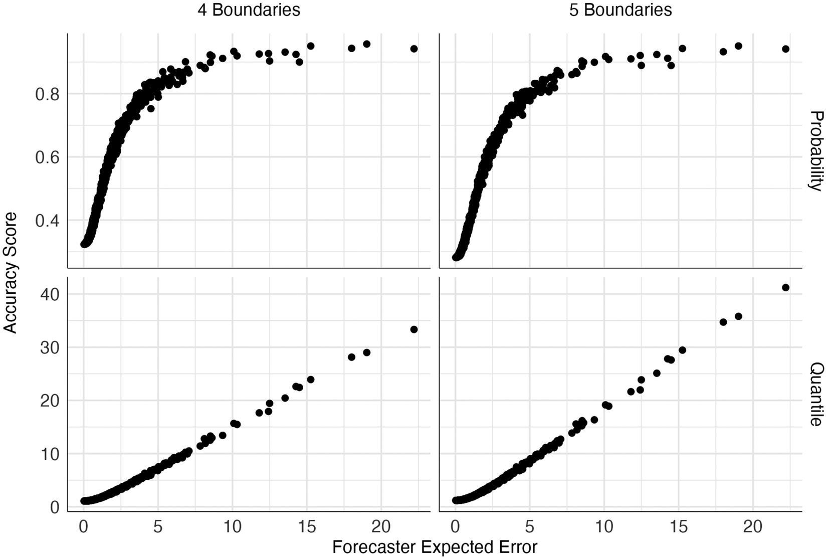
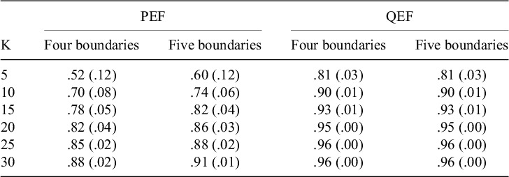
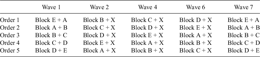
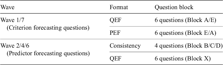
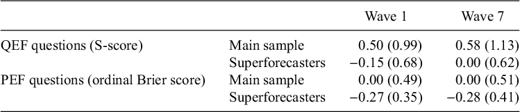
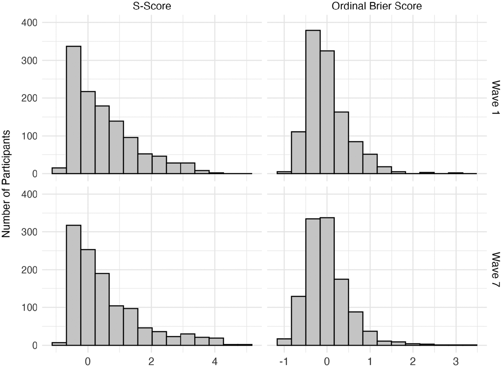

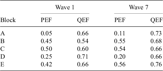
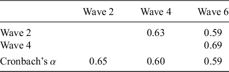
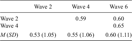
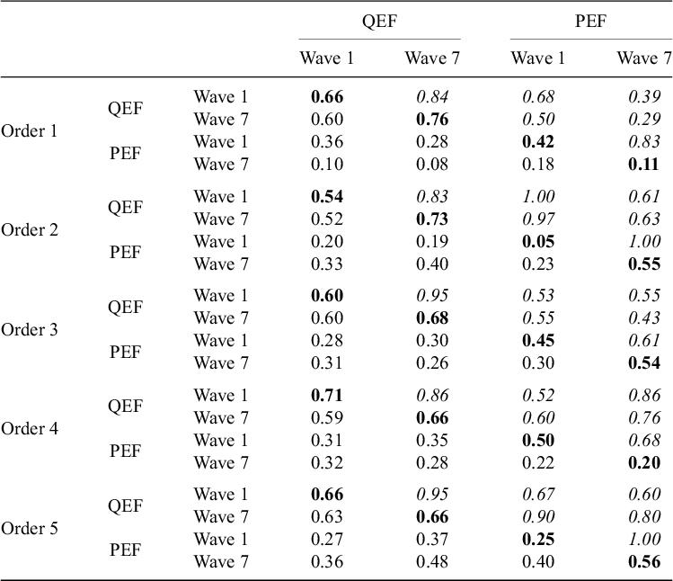
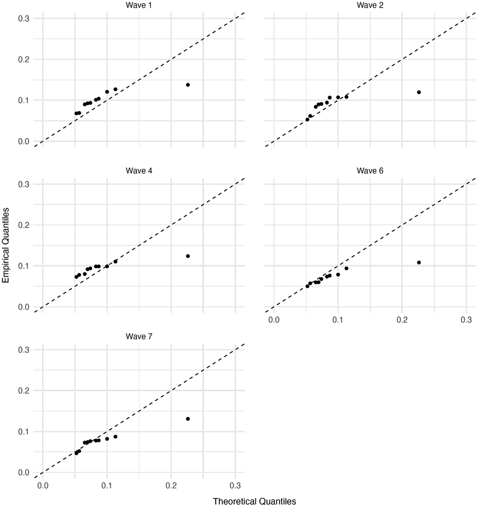
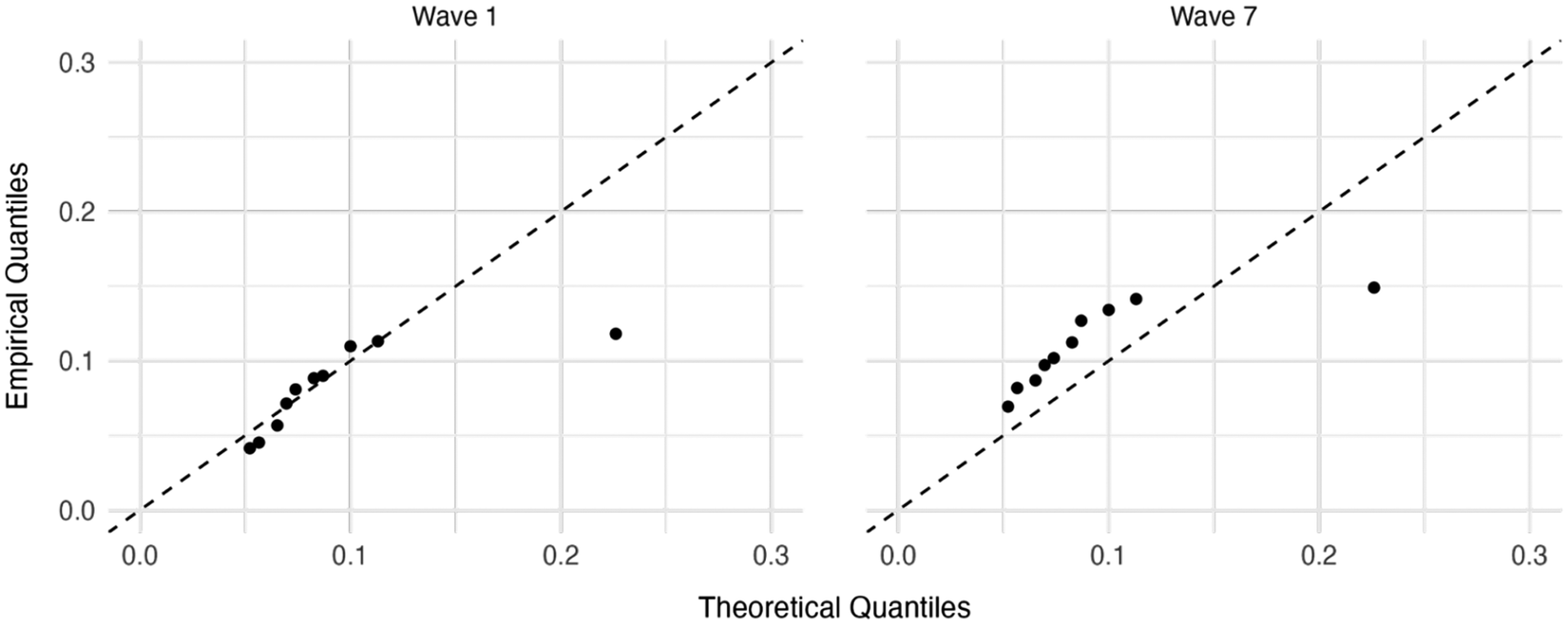
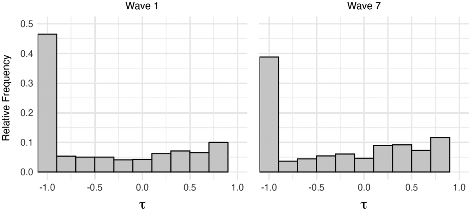
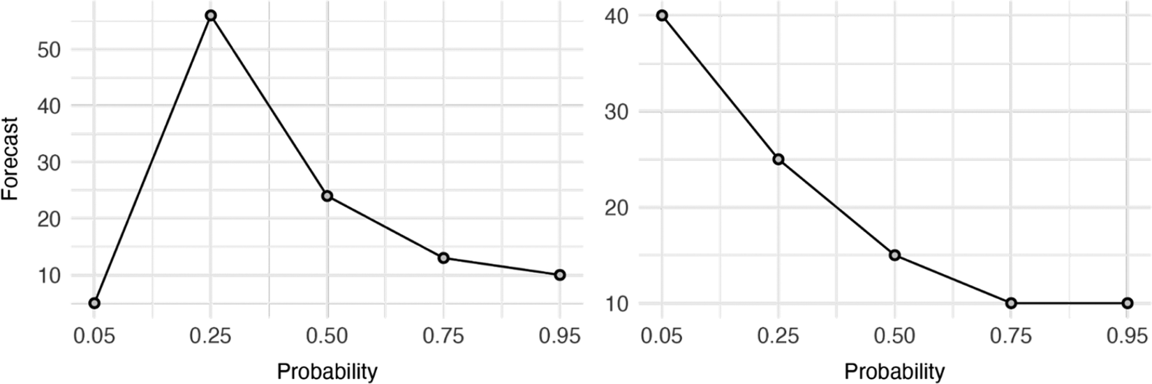


 Open access

