





Nomenclature
- ASTM
-
American Society for Testing and Materials
- ATJ
-
alcohol-to-jet
- CCW
-
sounterclockwise
- CW
-
slockwise
- DCN
-
Derived Cetane Number
- DLR
-
German Aerospace Center
- EDC
-
eddy dissipation concept
- EICO
-
CO emission index
-
 $\mathrm{EINO_x}$
-
$\mathrm{NO_x}$
emission index
- ESF
-
Eulerian stochastic fields
- FM
-
fractal model
- FRC
-
finite rate chemistry
- GC
-
gas chromatography
- H/C
-
hydrogen-to-carbon ratio
- IRZ
-
inner recirculation zone
- LBO
-
lean blow-out
- LDI
-
lean direct injection
- LDKM
-
localised dynamic
$k$
-equation model - LES
-
large eddy simulation
- NJFCP
-
National Jet Fuel Combustion Program
- NSRD
-
National Standard Reference Data Series
- NTC
-
negative temperature coefficient
- ODE
-
ordinary differential equation
- PaSR
-
partially stirred reactor
-
probability density function
- PISO
-
pressure-implicit with splitting of operators
- PIV
-
particle imaging velocimetry
- PLIF
-
planar laser-induced fluorescence
- RANS
-
Reynolds-averaged Navier–Stokes
- SAF
-
sustainable aviation fuels
- SMD
-
Sauter mean diameter
- TARS
-
triple annular research swirler


Roman symbol
-
$a_{mean}$
-
mean strain rate
-
$d$
-
droplet diameter
-
$D$
-
nozzle diameter
-
$D_{outlet}$
-
outlet diameter
-
$\Delta h_c$
-
specific enthalpy of combustion
-
$k$
-
subgrid turbulent kinetic energy
-
$L$
-
combustion chamber length
-
$\dot {m}$
-
mass flow rate
-
$n$
-
Rosin-Rammler distribution spread factor
-
$p$
-
pressure
-
$p_v$
-
vapour pressure
-
$\Delta p/p$
-
pressure drop
-
$\dot {Q}$
-
volumetric heat release rate
-
$r$
-
radial coordinate
-
$R^2$
-
coefficient of determination
-
$Re$
-
Reynolds number
-
$s_u$
-
unstretched laminar flame speed
-
$T$
-
temperature
-
$u$
-
velocity component
-
$U_{bulk}$
-
bulk velocity at nozzle exit
-
$W$
-
combustion chamber width
-
$x$
-
axial coordinate
-
$Y$
-
mass fraction
-
$Z$
-
mixture fraction


Greek symbol
-
$\alpha$
-
thermal diffusivity
-
$\gamma ^*$
-
turbulence-chemistry interaction scaling factor
-
$\varepsilon$
-
dissipation
-
$\theta$
-
circumferential coordinate
-
$\nu$
-
knematic viscosity
-
$\rho$
-
density
-
$\sigma$
-
surface tension
-
$\tau$
-
burner residence time
-
$\tau _c$
-
chemical timescale
-
$\tau _{ev}$
-
evaporation timescale
-
$\tau _{ig}$
-
ignition delay time
-
$\tau _K$
-
Kolmogorov timescale
-
$\tau _m$
-
mixing timescale
-
$\tau _p$
-
subgrid turbulent kinetic energy dissipation timescale
-
$\phi$
-
equivalence ratio


Mathematical symbol
-
$\langle \ \rangle$
-
time average
-
$\overline {\ \ \ }$
-
azimuthal or planar average


Subscripts
-
$air$
-
air
-
$b$
-
burnt
-
$boil$
-
boiling
-
$fuel$
-
fuel
-
$g$
-
global
-
$gas$
-
gas
-
$l$
-
liquid
-
$10,\ 90$
-
percentage recovered during distillation
-
$u$
-
unburnt
-
$\tau$
-
burner-relevant timescale


1.0 Introduction
The aviation industry is expanding at a rapid pace: in 2024, the International Air Transport Association reported surpassing the previous 2019 record in passenger traffic, with a projected increase in demand [1]. At the same time, several legislative initiatives, such as the RefuelEU Aviation Regulation, are promoting the increased use of sustainable aviation fuels (SAF) for reducing the carbon footprint of air travel. The chemical and physical properties of certified SAF comply with the narrow ranges defined by ASTM International standards [2]; however, their unique characteristics can impact the infrastructure network and may also affect engine performance, e.g. emissions, lean blow-out (LBO) limits and combustion stability [Reference Ruan, Yu and Lu3].
In assessing the combustion behaviour of candidate fuels, engineers and researchers rely on experimental and numerical investigations of increasing complexity, intended as pre-screening tools before entering the formal ASTM D4054 evaluation process [Reference Heyne, Rauch, Le Clercq and Colket4]. At first, the composition of fuel samples is measured using spectroscopic techniques and gas chromatography (GC). The outcome of those measurements is used to predict physical properties using statistical models [Reference Vozka and Kilaz5]. Subsequently, global combustion parameters, such as laminar burning velocity and ignition delay time, are measured in laboratory burners and shock tubes [Reference Richter, Kukkadapu, Westbrook, Braun-Unkhoff, Naumann, Köhler and Riedel6–Reference Luecke, Naser, Yang, Heyne and McCormick8], and their values are used as a reference for chemical kinetics modelling. Combustion testing typically continues to experimental rigs capable of mimicking the main physical features of real combustors, offering insight into the turbulent combustion process.
An example of such a test platform was the referee rig, a single-cup swirl-stabilised combustor introduced in the context of the National Jet Fuel Combustion Program (NJFCP). The campaigns were key milestones in demonstrating the importance of both physical and chemical properties on LBO [Reference Colborn, Heyne, Stouffer, Hendershott and Corporan9] and other operating conditions. The combustor responded non-monotonically to fuel properties and pressure drop,
 $\Delta p/p$
. While physical properties dominated at low pressure drop, ignition properties became relevant at high
 $\Delta p/p$
. Follow-up studies [Reference Boehm, Colborn and Heyne10] extended the analysis to a large set of combustors, including a GE9X full annular rig. It was found that trends became consistent if the relative ratios of timescales – atomisation, evaporation, mixing and ignition – were taken into account. This confirmed the value of representative geometries in gaining information on the combustion behaviour of fuel candidates at various operating conditions. Non-dimensional parameters and fuel properties, such as the Ohnesorge number, vapour pressure and the derived cetane number (DCN), were used to estimate the timescale similarity.
Alongside experimental testing, numerical studies [Reference Esclapez, Ma, Mayhew, Xu, Stouffer, Lee, Wang and Ihme11–Reference Shastry, Riber, Gicquel, Cuenot and Bodoc14] provided valuable insight into flow, flame structure, stabilisation and blow-out mechanisms. Simulations supported the concurrent effects of physical and chemical processes and showed partial agreement in the identification of design-relevant fuel trends. Generally, authors recognised the many modelling challenges and uncertainties, highlighting the importance of appropriate sensitivity studies with respect to the sub-models.
In this context, the present numerical study targets the in-house, single-cup, swirl-stabilised atmospheric rig with the goal of investigating its fuel sensitivity under two distinct families of chemical reaction mechanisms. The impact of chemical kinetics on the simulation results is assessed through cross-analysis of the fuel trends. The paper is organised as follows. Section 2 gives an overview of the experimental and simulation setup, the composition and properties of the fuels and combustion chemistry. Section 3 provides validation of the simulation methodology and discusses the results. Section 4 summarises the main conclusions.
(a) Detail of the triple annular research swirler. (b) Combustion chamber in the atmospheric combustion test facility. (c) Mesh used in the numerical simulations.

Figure 1. Long description
Panel A: A detailed view of the triple annular research swirler, showing the inner, intermediate, and outer swirlers. Panel B: A diagram of the combustion chamber in the atmospheric combustion test facility, highlighting components such as the steel structure, quartz windows, dome, TARS, plenum, and the inlet for pre-heated air. Panel C: A depiction of the mesh used in numerical simulations, indicating it consists of 18 million elements.
2.0 Triple annular research swirler
The experimental facility is equipped with the triple annular research swirler (TARS), whose digital mock-up is shown in Figure 1a. It features three concentric swirlers with two fuel injection paths in the outer and intermediate swirler channels. The injector was designed by Delevan Gas Turbine Products to explore the concept of variable nozzle geometry. Early studies [Reference Li and Gutmark15–Reference Li and Gutmark17] focused on characterising different flow patterns, combustion characteristics and the effect of the area ratio at the combustion chamber exit section. Later, the burner was further studied experimentally and numerically in a non-reactive scenario [Reference Umeh, Rusak, Gutmark, Villalva and Cha18]. The results showed good agreement between particle imaging velocimetry (PIV) measurements and Reynolds-averaged Navier-Stokes (RANS) simulations. Subsequently, reacting cases were studied with different swirler designs [Reference Iudiciani, Hosseini, Szasz, Duwig, Fuchs, Collin, Lantz, Aldén and Gutmark19], with gaseous propane and a premixing section [Reference Umeh, Rusak and Gutmark20], and in lean direct injection (LDI) configuration [Reference Villalva, Umeh, Murugappan and Gutmark21]. Additionally, the stability of the swirling flame was studied using proper orthogonal decomposition [Reference Iudiciani, Duwig, Hosseini, Szasz, Fuchs and Gutmark22], and active control strategies were investigated at close-to-LBO conditions [Reference Li, Zhou, Jeffries and Hanson23]. The burner was also the object of numerical studies. The non-reacting and reacting TARS flows were modelled using large eddy simulation (LES) and a flame-wrinkling model, achieving satisfactory agreement with experimental data [Reference Fureby, Grinstein, Li and Gutmark24] and validating the use of LES for similar studies. Later, the flow details inside the swirler were investigated in a separate study [Reference Iudiciani, Duwig, Hosseini, Szasz, Fuchs and Gutmark25] using LES. Recently, the burner was simulated, focusing on SAF effects [Reference Vauquelin, Cakir, Sanned, Prakash, Hannappel, Subash, Richter, Bai and Fureby26]. The recent study constitutes the basis of the present work.
Several vane angle choices are available for the outer, intermediate and inner swirlers. The configuration used in the present study employs co-rotating outer and intermediate swirlers, each with eight 45
 $^\circ$
vanes in a counterclockwise (CCW) orientation, while the inner swirler features four 55
 $^\circ$
vanes rotating clockwise (CW). The TARS, whose nozzle diameter is
 $D = 50.8\, \mathrm{mm}$
, is flush-mounted on a
 $400\, \mathrm{mm}$
-long, square
 $140\times 140\,\mathrm{mm}^2$
cross-section combustion chamber, transitioning into a circular outlet (
 $D_{outlet}=80\, \mathrm{mm}$
) through a convergent section, as in Figure 1b. The rig can be equipped with various optical diagnostics setups, as well as exhaust gas emissions measurements, with the aim of addressing fuel-dependent trends among different fossil and alternative aviation fuels.
2.1 Simulation setup
Parallel to the experiments and with analogous scopes, the LES of the rig follow the OpenFOAM-based methodology outlined and validated in previous work. The methodology was used to study an industrial gas turbine combustor [Reference Bulat, Fedina, Fureby, Meier and Stopper27, Reference Fedina, Fureby, Bulat and Meier28] and lab-scale burners, both bluff-body stabilised [Reference Åkerblom, Zettervall and Fureby29, Reference Åkerblom and Fureby30] and swirl-stabilised [Reference Ercole and Fureby31]. Additionally, the approach has been recently employed and validated in non-premixed, spray cases of aeronautical interest [Reference Vauquelin, Cakir, Sanned, Prakash, Hannappel, Subash, Richter, Bai and Fureby26, Reference Åkerblom and Fureby32].
The modelling framework is based on the OpenFOAM built-in multiphase reacting flow solver, based on spatially filtered, unsteady, compressible transport equations for mass, momentum, energy and chemical species mass fractions. The thermodynamic state of the mixture is closed using the state equation for an ideal gas. Diffusive fluxes of mass and heat are closed using Fick and Fourier diffusion models with constant Prandtl and Schmidt numbers and assuming a unity Lewis number. Sub-grid turbulence is taken into account using the localised dynamic
 $k$
-equation model (LDKM) of Kim and Menon [Reference Kim and Menon33], and near-wall turbulence is modelled using a wall model based on Spalding’s law of the wall [Reference Spalding34]. Turbulence-chemistry interaction is closed with the partially stirred reactor (PaSR) model [Reference Sabelnikov and Fureby35], previously assessed in LES of premixed and non-premixed burners [Reference Fedina, Fureby, Bulat and Meier28, Reference Åkerblom and Fureby32]. In the last study, other models – namely the fractal model (FM), eddy dissipation concept (EDC) and Eulerian stochastic fields (ESF) – were compared with PaSR; the study determined better agreement for PaSR and ESF. Given the higher computational cost of the second, the first is selected for the current study. The model compares chemical and mixing timescales to provide a scaling factor for the reaction rates,
 $\gamma ^*=\tau _c/(\tau _c+\tau _m)$
. The chemical timescale is selected globally and a priori using thermal diffusivity of the reactants and laminar burning velocity of the mixture at the global equivalence ratio,
 $\tau _c=\alpha /s_u^2$
. Defining molecular viscosity,
 $\nu$
, subgrid turbulent kinetic energy,
 $k$
, and dissipation,
 $\varepsilon$
, the mixing timescale is obtained from
 $\tau _m=\sqrt {\tau _K\tau _p}$
, where
 $\tau _K=\sqrt {\nu /\varepsilon }$
is the Kolmogorov timescale and
 $\tau _p=k/\varepsilon$
is the timescale of subgrid turbulent kinetic energy dissipation. The scaling factor
 $\gamma ^*$
is then applied to the reaction rates obtained by locally solving the stiff ordinary differential equation (ODE) system using an extrapolation algorithm based on the linearly implicit Euler method known as SEULEX [Reference Hairer, Nørsett and Wanner36]. This direct integration approach with an operator-splitting procedure is often referred to as finite rate chemistry (FRC) [Reference Fedina, Fureby, Bulat and Meier28].
Due to the prohibitive cost of resolving primary break-up, the fuel is presumed fully atomised at injection following the approach proposed by Dukowicz and Reitz [Reference Dukowicz37, Reference Reitz38]. Each Lagrangian parcel represents a collection of fuel droplets with identical properties. These are tracked along their trajectory as they break up, evaporate and mix with the turbulent flow. The diameter at injection follows a Rosin-Rammler distribution with characteristic diameter
 $d=9\,\mu \mathrm{m}$
, minimum and maximum diameters
 $d_{min}=1\,\mu \mathrm{m}$
and
 $d_{max}=20\,\mu \mathrm{m}$
and spread parameter
 $n=2.5$
. The probability distribution is identical to that used in LES of the single-cup DLR combustor at idle conditions [Reference Åkerblom and Fureby32], reported in Figure 5. The injection model was then matched to experimental droplet sizing downstream in the combustion chamber, based on a previous study [Reference Jones, Marquis and Vogiatzaki39]. It follows that the set of parameters does not physically represent droplet size at the injection location, but rather a boundary condition yielding good agreement with experimental data in analogous simulations, justifying its use as a starting guess in the current modelling effort.
After injection, the model of Reitz and Diwakar [Reference Reitz and Diwakar40] is used for secondary break-up, while the model of Ranz and Marshall [Reference Ranz and Marshall41] is used to model heat transfer. The evaporation model accounts for both standard liquid evaporation and the more rapid boiling process. Additionally, the 19-step mechanism from Yoshikawa and Reitz [Reference Yoshikawa and Reitz42] is employed to predict
 $\mathrm{NO}_x$
emissions from both the thermal and prompt pathways. Section 2.3 is dedicated to providing details on the kinetic schemes used throughout the study.
Air at
 $T_u=450\,\mathrm{K}$
enters the domain in the plenum with a mass flow rate of
 $\dot {m}_{air}=26\,\mathrm{g/s}$
, corresponding to a Reynolds number
 $Re\approx 26\,000$
. Fuel is injected from the 12 ports (8 in the outer swirler channel, 4 in the intermediate swirler). Overall, the injection sites feed
 $\dot {m}_{fuel}\approx 1.1\,\mathrm{g/s}$
at a temperature
 $T_l=293\,\mathrm{K}$
, with small mass flow rate variations between fuels to keep the thermal load constant. This results in a lean global equivalence ratio of
 $\phi _g\approx 0.6$
. Table 1 summarises the key settings for the three fuels.
Operating conditions for the three fuel cases

Table 1. Long description
A table comparing operating conditions for three fuel cases: Jet A, C1, and C5. The table has 4 rows and 4 columns. Column headers are: Jet A, C1, and C5. Row labels are: m_dot_air (g/s), m_dot_fuel (g/s), total, T_t (K), and T_t (K). Row 1: m_dot_air (g/s), 26.00, 26.00, 26.00. Row 2: m_dot_fuel (g/s), total, 1.0656, 1.0710, 1.0831. Row 3: T_t (K), 450, 450, 450. Row 4: T_t (K), 293, 293, 293.
Figure 1c shows the computational domain, discretised with an eighteen-million volumes tetrahedral mesh including part of the plenum, the swirler and the full combustion chamber. Significantly lower resolution levels were sufficient to satisfactorily model the main flow structures in previous studies [Reference Fureby, Grinstein, Li and Gutmark24]. Nonetheless, the newly generated mesh was locally refined to better resolve the partially premixed flame front. Each iteration was based on the statistical position of the flame in the LES results. At the current resolution level, the cell size in the flame region is approximately the thermal thickness of the corresponding premixed flame at the global
 $\phi =0.6$
. This represents a commonly accepted compromise in the LES-PaSR approach. Finally, it is important to mention that the smallest cell size is found inside the swirler, in a region of high flow velocity. This limits the timestep to
 $\Delta t\approx 2\times 10^{-7}\,\mathrm{s}$
, and challenges the use of higher resolutions, especially in the FRC context.
Non-adiabatic boundary conditions are used at the combustion chamber sidewalls, using estimated material-specific values in the evaluation of the conductive thermal fluxes through the walls. At the dome, a fixed temperature value of
 $800\,\mathrm{K}$
is used instead. Pressure is fixed at the inlet together with the mass flow rate, while the outlet boundary condition allows acoustic waves to propagate, preventing the build-up of standing pressure waves that would affect flame dynamics. The equations are solved using a finite volume method and pressure-velocity coupling (pressure-implicit with splitting of operators (PISO) algorithm). Gradients are obtained using a least-squares scheme, while convective fluxes are reconstructed using monotonicity-preserving limiters; central differencing with non-orthogonal correction is used for the diffusive fluxes. Time advancement is performed using the first-order implicit Euler method, keeping the maximum Courant number in the domain below 0.8. Finally, a dynamic load balancing algorithm [Reference Tegkül, Peltonen, Kahila, Kaario and Vuorinen43, Reference Morev, Tekgül, Gadalla, Shahanaghi, Kannan, Karimkashi, Kaario and Vuorinen44] was used to reduce the computational cost of FRC using the more complex HyChem reaction mechanisms. This allowed the computational cost of those simulations to stay at
 $\approx 25\,000 \pm 5\,000\,$
core-h/ms, compared to the cost of Z79 simulations, i.e.
 $\approx 12\,000\,$
core-h/ms. The simulations were performed on 768 or 1024 processors, using several machines. All simulations were time-averaged over
 $15\,\mathrm{ms}$
.
2.2 Composition and properties of the fuels
The fuels of interest – namely Jet A, C1, and C5 – are included in two different categories following the classification outlined in the NJFCP. In particular, Jet A is part of the so-called Category A, while C1 and C5 are part of Category C. The former includes conventional fossil jet fuels, such as Jet A (civil aviation) and JP-5 or JP-8 (military grades). These fuels comply with the standard range of chemical composition, thermophysical, spray and combustion properties for jet fuels. On the other hand, Category C consists of experimental test fuels designed to push the envelope of jet fuel properties for research purposes.
The composition of the three fuels is reported in Table 2, distinguishing among different hydrocarbon groups. Noticeably, C1 and C5 show differences with Jet A in terms of aromatics content and various groups of paraffins. The alternative fuel C1 is a neat alcohol-to-jet (ATJ) synthetic fuel, and is notable for its low aromatics content. Besides, the predominance of highly branched iso-paraffins results in a fuel of low reactivity, quantified by the low DCN of Table 3. Finally the laboratory fuel C5, only consisting of
 $\mathrm{C}_{10}$
/
 $\mathrm{C}_{11}$
n- and iso-paraffins and 1,3,5-trimethylbenzene, is characterised by a flat boiling curve, as highlighted by the low
 $T_{90} - T_{10} = 2.9\,\mathrm{K}$
. In addition to reactivity and evaporation properties, other bulk properties, such as density and viscosity, are affected by the differences in composition. As will be discussed in the following, this has effects on the behaviour of the spray cloud, and on the combustion behaviour of the three fuels [Reference Esclapez, Ma, Mayhew, Xu, Stouffer, Lee, Wang and Ihme11, Reference Stouffer, Hendershott, Monfort, Diemer, Corporan and Wrzenski45].
Composition of conventional Jet A, C1 and C5. Data adapted from [Reference Esclapez, Ma, Mayhew, Xu, Stouffer, Lee, Wang and Ihme11]

Table 2. Long description
A table with three rows and six columns comparing the molecular weight and composition of three fuels: Jet A, C1, and C5. The columns are labeled Mol. weight (kg/kmol), Arom. (percent), iso-par. (percent), n-par. (percent), cyclo-par. (percent), and Olefins (percent). Row 1: Jet A, Mol. weight 158.6, Arom. 23.42, iso-par. 26.09, n-par. 19.33, cyclo-par. 31.16, Olefins -. Row 2: C1, Mol. weight 178, Arom. 99.63, iso-par. 0.05, n-par. 0.32, cyclo-par. -, Olefins -. Row 3: C5, Mol. weight 135.4, Arom. 34.38, iso-par. 48.90, n-par. 16.72, cyclo-par. -, Olefins -.
Properties of Jet A, C1 and C5. Data adapted from [Reference Edwards50] and [Reference Esclapez, Ma, Mayhew, Xu, Stouffer, Lee, Wang and Ihme11]

Table 3. Long description
A table comparing properties of Jet A, C1, and C5 fuels. The table has 3 rows and 6 columns. Column headers are H/C, Δh_c (MJ/kg), DCN, T_10 (K), T_90 - T_10 (K), and ρ (kg/m^3). Row 1: Jet A, 1.90, 43.1, 48.3, 450, 67.8, 803. Row 2: C1, 2.16, 43.8, 17.1, 452.1, 42.5, 760. Row 3: C5, 1.93, 43.0, 39.6, 434.7, 2.9, 769.
2.3 Combustion chemistry
A well-known difficulty of SAF combustion modelling resides in its complex reaction mechanisms, which must be reduced for use in LES. This process results in families of kinetic schemes from different research groups that typically differ in their prediction of fundamental combustion properties. Here, we focus on the comparison between the pathway-centric Z79 mechanisms by Zettervall [Reference Åkerblom, Zettervall and Fureby29], and the HyChem mechanisms [Reference Xu, Wang, Banerjee, Shao, Parise, Zhu, Wang, Movaghar, Lee, Zhao, Han, Gao, Lu, Brezinsky, Egolfopoulos, Davidson, Hanson, Bowman and Wang46]. The six mechanisms target the three fuels of Section 2.2. The average formula for Jet A is
 $\mathrm{C}_{11}\mathrm{H}_{22}$
, while the two Cat. C fuels, C1 and C5, are globally described as
 $\mathrm{C}_{13}\mathrm{H}_{28}$
and
 $\mathrm{C}_{10}\mathrm{H}_{19}$
, respectively.
Figure 2 shows a schematic of the two modelling frameworks. In general, both approaches reduce the number of reactions in fuel thermal decomposition and rely on more detailed schemes for oxidation kinetics of decomposition products. For this task, the USC Mech IIa is used in the three HyChem mechanisms. Major differences are found in the modelling of fuel decomposition. In the C1 and C5 mechanisms, the fuel molecule undergoes a seven-step high-temperature decomposition as outlined in Figure 2. This produces a variety of species that are then consumed in the foundational block. On the other hand, the selected Jet A mechanism accounts for both high-temperature decomposition and low-temperature fuel oxidation, following the canonical reaction pathways [Reference Curran, Gaffuri, Pitz and Westbrook47]. This gives a more faithful representation of low-temperature ignition behaviour, as discussed in the following. Similarly, Z79 includes an eight-step low-temperature oxidation pathway, but with differences in the fuel, alkyl radical, ketone and olefin decomposition and oxidation products. Indeed, Z79 connects the fuel breakdown block to a highly reduced C
 $_2$
block (22 irreversible reactions), providing radicals to a compact but comprehensive H/C/O block (43 irreversible reactions). After including the NO
 $_x$
submodel mentioned in Section 2.1, the three Z79 mechanisms contain 37 species and 98 irreversible reactions. On the other hand, the HyChem mechanisms all contain more than 48 species and 219 reactions, as from Figure 2. It is important to mention that the resulting mechanisms share the same thermophysical gas properties for the fuel species, H
 $_2$
O, CO
 $_2$
and for more than 20 other species involved in C
 $_2$
, H/C/O and NO
 $_x$
chemistry.
Description of the HyChem and Z79 modelling frameworks.

Global combustion parameters for the Z79 (dashed) and HyChem (solid) families of reaction mechanisms. (a) Flame temperature, and (b) laminar flame speed, at
 $T_u=400\,\mathrm{K}$
. (c-d) Ignition delay time at stoichiometric conditions, for atmospheric pressure and
 $p=10\,\mathrm{bar}$
. Data from Xu et al. [Reference Xu, Wang, Banerjee, Shao, Parise, Zhu, Wang, Movaghar, Lee, Zhao, Han, Gao, Lu, Brezinsky, Egolfopoulos, Davidson, Hanson, Bowman and Wang46], and Wang et al. [Reference Wang, Xu, Parise, Shao, Movaghar, Lee, Park, Gao, Lu, Egolfopoulos, Davidson, Hanson, Bowman and Wang48, 49]. (e) Surface tension and (f) vapour pressure of the three fuels across temperature. Fit to measurements from Edwards [Reference Edwards50].

Figure 3. Long description
Panel A: A line graph shows flame temperature (T_b) in Kelvin (K) against equivalence ratio (phi). The graph includes multiple data series for different fuels and mechanisms: HyC - Jet A, Z79 - Jet A, HyC - C1, Z79 - C1, HyC - C5, and Z79 - C5. Panel B: A line graph displays laminar flame speed (s_u) in meters per second (m/s) against equivalence ratio (phi). Data series are labeled similarly to Panel A, with additional data points from Xu 2018 - Jet A, Wang 2018 - C1, and Wang - C5. Panel C: A line graph illustrates ignition delay time (tau_ign) in seconds (s) against the inverse of temperature (1000/T) in Kelvin (K). The graph includes data series for different fuels and mechanisms at stoichiometric conditions and atmospheric pressure. Panel D: Another line graph shows ignition delay time (tau_ign) in seconds (s) against the inverse of temperature (1000/T) in Kelvin (K) for different pressures: Xu 2018 - Jet A, 12 bar; Wang 2018 - C1, 11 bar; Wang - C5, 11.9 bar. Panel E: A line graph presents surface tension (sigma) in Newtons per meter (N/m) against liquid temperature (T_l) in Kelvin (K) for three fuels. Panel F: A line graph depicts vapor pressure (p_v) in Pascals (Pa) against liquid temperature (T_l) in Kelvin (K) for three fuels, with data from Edwards 2017 - A2, C1, and C5.
Figure 3 highlights the differences in the predictions of fundamental combustion properties. At unburnt temperature
 $T_u=400\,\mathrm{K}$
and varying equivalence ratio,
 $\phi$
, the 1D, premixed flame temperature,
 $T_b$
, is predicted with good precision (see Figure 3a). In terms of laminar flame speed,
 $s_u$
, C1 shows the lowest values, while Jet A and C5 show comparable results. Overall, Figure 2b suggests good agreement with experimental data [Reference Xu, Wang, Banerjee, Shao, Parise, Zhu, Wang, Movaghar, Lee, Zhao, Han, Gao, Lu, Brezinsky, Egolfopoulos, Davidson, Hanson, Bowman and Wang46, Reference Wang, Xu, Parise, Shao, Movaghar, Lee, Park, Gao, Lu, Egolfopoulos, Davidson, Hanson, Bowman and Wang48, 49]. It can be noticed how values for
 $s_u$
tend to be more consistent between the two families of reaction mechanisms at lean equivalence ratios, while larger discrepancies are found at rich conditions. This feature can be explained by the rate-limiting processes involved in the propagation of lean and rich flames. Lean flames are governed by radical formation and base chemistry (H/C/O) and are therefore described more accurately. On the other hand, rich conditions are constrained by fuel decomposition pathways, which are more case-dependent, as previously discussed.
Results for ignition delay time,
 $\tau _{ig}$
, show the largest discrepancies. In Figure 3c-d,
 $\tau _{ig}$
is defined as the time delay after which the temperature of the 0D reactor has risen
 $300\,\mathrm{K}$
above the initial temperature. The kinetic simulations are performed at
 $p=1\,\mathrm{atm}$
and
 $p=10\,\mathrm{atm}$
, and
 $\phi =1.0$
. Experimental datapoints at similar conditions are reported in Figure 3d for reference. At low temperature, the three Z79 and the HyChem Jet A mechanisms show evidence of negative temperature coefficient (NTC) behaviour, while HyChem C1 and C5 do not exhibit it. This phenomenon, caused by the shifting balance between chain propagation and chain branching paths in favour of the first [Reference Curran, Gaffuri, Pitz and Westbrook47], is particularly important in non-premixed combustion since it influences the prediction of relevant characteristics such as lift-off length and flame dynamics. Following the discussion of Figure 2, the inclusion of low-temperature oxidation pathways in HyChem Jet A and Z79 allows for a better description of low-temperature ignition behaviour. At higher temperatures, i.e. around
 $1250\,\mathrm{K}$
, the mechanisms show consistent trends in fuel reactivity, and the separation between the least and most reactive fuels, i.e. C1 and Jet A, spans almost one order of magnitude as visible in the inset of Figure 3c. This follows the compositional portrait of Table 2: because of the high content of branched iso-paraffin, C1 decomposes more slowly; on the other hand, Jet A and C5 have higher n-paraffin content, and this makes them ignite faster and more alike in terms of reactivity.
The structures of premixed and non-premixed flames, calculated in Cantera, are presented in Figure 4. The temperature distribution is shown alongside the mass fractions of OH, CO and NO. The data include two premixed flames at
 $T_u=450\,\mathrm{K}$
, with
 $\phi =0.6$
and
 $\phi =1.0$
, and a counter-flow diffusion flame of fuel/N
 $_2$
in O
 $_2$
with
 $\dot {m}_{fuel}/\dot {m}_{\mathrm{N}_2}=0.09$
, and
 $T=450\,\mathrm{K}$
for both streams. In the stoichiometric premixed case, the mechanisms are compared with the detailed kinetics from the CRECK group [Reference Ranzi, Cavallotti, Cuoci, Frassoldati, Pelucchi and Faravelli51] for Jet A and ATJ surrogates. The largest differences are found in the oxidation layer and in the post-flame zone. Mechanisms of the HyChem family predict a faster temperature increase, more in line with the detailed kinetics. On the other hand, Z79 better matches the detailed hydroxyl radical recombination and CO oxidation. Furthermore, Figure 4 suggests that NO
 $_{\mathrm{x}}$
sub-mechanism gives a good estimate of the NO production rates. The diffusion flame structure shows similar results: in the Z79 cases, CO is found at higher mass fractions on the fuel side of the flame, and NO reaches higher peak values. These discrepancies can be explained by differences in the fuel decomposition and base chemistry of the two groups of mechanisms and are likely to explain some of the variations in the LES results presented later.
Comparison of flame structures for the reaction mechanisms of interest. The first and second rows show
 $T$
,
 $Y_{OH}$
,
 $Y_{CO}$
and
 $Y_{NO}$
for a lean (
 $\phi =0.6$
) and stoichiometric freely propagating flame. The third row shows results for a counter-flow diffusion flame at
 $\dot {m}_{fuel}/\dot {m}_{\mathrm{N}_2}=0.9$
, with both streams at
 $T=450\,\mathrm{K}$
and mean strain rate of
 $a_{mean}=1.2\,\mathrm{s}^{-1}$
.

In the present study, we perform full-scale simulations with both families of reaction mechanisms for the three fuels, resulting in a total of six cases. The goal is to cross-validate fuel trends by isolating the choice of chemical kinetics. Similarly, fuel-specific liquid properties [Reference Åkerblom, Passad, Ercole, Zettervall, Nilsson and Fureby52] are used to incorporate the different atomisation properties and volatility of the fuels. For example, Figure 3e and f show surface tension and vapour pressure in their variation with the liquid temperature,
 $T_l$
, across the different fuels. Those and other liquid properties are kept consistent across different chemical kinetics, i.e. simulations of the same fuels using different reaction mechanisms share the fit to the data of Edwards [Reference Edwards50].
Before discussing the results, Figure 5 is presented to assess the potential impact of the liquid properties, droplet diameter and air temperature on the LES results. The figure shows the evaporation time,
 $\tau _{ev}$
, of isolated droplets with different initial diameters, in quiescent air at
 $T_{gas}=350,\ 450,\ 550\,\mathrm{K}$
. The timescale is calculated by tracking the liquid mass fraction in the gaseous phase, and selecting the time at which the mass fraction reaches 99% of its final value. The simulations are performed in the same framework, using identical liquid properties and mass-heat transfer models to the 3D LES. The injection probability distribution at the 12 TARS injection ports is reported for reference. Evaporation, i.e.
 $\tau _{ev}$
, follows the well-known
 $d^2$
-law, suggesting a strong, non-linear sensitivity to the injection distribution, which surpasses fuel variations for small uncertainties in the probability density function (PDF). In general, smaller droplets and faster evaporation would shift combustion towards a premixed regime, a fact that must be carefully considered if tabulated combustion modelling is performed based on non-premixed configurations. However, in the multi-regime approach used in this work, assumptions on droplet sizing do not compromise the applicability of the combustion models. Finally, for the selected distribution and
 $T_{gas}=450\,\mathrm{K}$
, isolated droplets up to approximately the Sauter mean diameter (SMD) evaporate within a burner-relevant residence time,
 $\tau =D/U_{bulk}\approx 3\,\mathrm{ms}$
. This suggests that the distribution, introduced in Section 2.1, represents a reasonable compromise for the objectives of the study, i.e. to assess the impact of different chemical reaction mechanisms and fuel properties.
Evaporation timescale of isolated droplets at three different temperature values. The same models as in the 3D LES have been used to perform the simulations. In grey, the injection probability distribution and its SMD.

Figure 5. Long description
Panel: A line graph with the horizontal axis labeled ‘d (μm)’ ranging from 0 to 20 and the vertical axis labeled ‘τ_ev (ms)’ ranging from 0 to 5. The graph includes multiple lines representing different conditions: Jet A, C1, and C5, with varying temperatures (350 K, 450 K, and 550 K). The lines show the evaporation timescale of isolated droplets at these temperatures. The grey line represents the injection probability distribution and its SMD. The lines for different conditions and temperatures show varying trends, with evaporation times generally increasing with droplet diameter.
3.0 Results and discussion
The discussion of the results focuses on two key aspects: the dependence of the results on the choice of the fuel, and their strong sensitivity to the reaction mechanism family, i.e. generally different results between Z79 and HyChem cases. In Section 3.1, the simulation results for the baseline Jet A - Z79 case are compared with the respective experiment. After, instantaneous LES flame structures are compared across fuels in Section 3.2, while Sections 3.3 and 3.4 describe the time-averaged numerical results in terms of axial-radial and axial distributions. Section 3.5 connects some engine-relevant trends with kinetic and physical properties, while a brief explanation of the impact of those on pollutant emissions is given in Section 3.6, where comparison with experimental data is also presented.
3.1 Validation measurements
To validate the numerical setup, experimental chemiluminescence images are compared to numerical volume renderings. Experiments at the operating conditions given in Table 1 were performed for the Jet A case with a locally sourced Jet A1, while the test fuels C1 and C5 could not be tested due to supply challenges. High-speed images were taken with a Photron SA-X2 high-speed camera, equipped with a Nikon AF MICRO-NIKKOR
 $105\,\mathrm{mm}$
objective. A shortpass filter with a cut-off wavelength of
 $650\,\mathrm{nm}$
was used to filter background radiation from the combustion chamber. A total of 2,001 images were taken at a frame rate of
 $10\,000$
frames per second and a shutter speed of
 $98.38\,\mathrm{\mu s}$
. The images were processed by first applying a threshold to exclude areas with strong radiation from soot. Afterwards, the 25-image minimum of each pixel was subtracted to remove the background. Through the application of the shortpass filter, the recorded images contain the chemiluminescence of the
 $\mathrm{CH^*}$
radical as well as the
 $\mathrm{C_2}$
species. Under the assumption that chemiluminescence is proportional to the mass fraction of
 $\mathrm{CH^*}$
, and that this one is proportional to
 $Y_{\mathrm{CH}}$
and
 $\dot {Q}$
, the scaled heat release rate can be considered a qualitative marker for the filtered flame radiation.
The upper row of Figure 6 shows three instantaneous snapshots from the Jet A experiments, and the resulting time average. Similarly, volume renderings of the volumetric heat release, weighted by CH mass fraction,
 $\dot {Q}\times Y_{\mathrm{CH}}$
, are shown for the Z79 - Jet A simulation. Figure 6b shows the spatial distribution of
 $\dot {Q}$
and
 $Y_{\mathrm{CH}}$
, together with the magnified spray cloud above the flush plane. The radical mass fraction forms more distributed structures than the heat release. However, the correlation between the two is strong, supporting the argument for estimating
 $\mathrm{CH^*}$
photon emission. Similarly, the Lagrangian parcels visualisation confirms that, according to the injection model and diameter distribution reported in Section 2.1, droplets are to be expected in the heat release region where the flame is experimentally imaged. The presence of droplets is connected to the case-specific test point. At the global equivalence ratio,
 $\phi _g=0.6$
, the mass flow rate was selected to limit the thermal load and ensure the chamber’s survival. Subsequent studies at lower
 $\phi$
and higher mass flow rates indicated that liquid droplets can be drastically reduced by increasing aerodynamic forces acting on the fuel jets at the injection ports. Analogous simulations to the ones presented here displayed good agreement with fuel and formaldehyde planar laser-induced fluorescence (PLIF). However, under the conditions of Table 1, the liquid fuel spray makes optical diagnostics more challenging, as noticeable in the experimental images of Figure 6.
Instantaneous and time-averaged flame structures from experiments and LES, for the Jet A case. Simulation data for the Z79 reaction mechanism. Burner axis placed vertically. On the right, visualisation of the superimposed heat release,
 $\dot {Q}$
, and CH mass fraction fields, shown together with the magnified spray cloud.

Figure 6. Long description
Panel A: Two rows of images side by side. The top row shows experimental flame structures, while the bottom row shows simulated flame structures using LES. Each row contains four images capturing different instances of the flame structures. The images depict the intensity of the CH* chemiluminescence signal. Panel B: A 3D visualization on the right side showing superimposed heat release rate and CH mass fraction fields. The heat release rate is represented by a color scale ranging from blue to yellow, and the CH mass fraction is shown in grayscale. The visualization includes a magnified view of the spray cloud at the bottom.
The instantaneous experimental images reveal localised, small-scale, high-intensity sources of signal linked to the atomisation process and to the presence of droplets. After the primary break-up, smaller droplets evaporate and mix fast. Conversely, larger ones penetrate deeper into the combustion chamber. There, they interact with the recirculated exhaust gas, quickly evaporate and combust at locally rich conditions, forming soot. This leads to chemiluminescence, as well as to high levels of broadband soot incandescence. If the local temperature is high enough, a fraction of the black-body radiation can still be captured by the detector, despite the shortpass filter at
 $650\,\mathrm{nm}$
(see Figure 6). The majority of soot is formed inside the flame on the left side of the field of view. At the same time, the chemiluminescence signal at lower intensity is still detectable at a larger scale in line with the LES results, which do not include any soot or radiation modelling.
The large-scale chemical structures are more clearly visible in time-averaged results, where information on fast, small-scale features, e.g. droplets and soot, is filtered away. In the last column of Figure 6, the LES captures relevant macroscopic features of the flame. The angle with the centreline and the visual structure match the experimental image. The three-lobed morphology has been observed in previous studies [Reference Li and Gutmark16, Reference Li and Gutmark17], and it is a direct consequence of the square cross-section combustion chamber coupled with the eight-plus-four injection system, Figure 1; this particular detail is also captured by the LES.
The strong left lobe visible in the experiments, and the general asymmetry of both the experimental and numerical results, is in line with observations from previous experimental campaigns with gaseous fuels [Reference Li and Gutmark16, Reference Li and Gutmark17]. Among the several factors, the imbalance could be attributed to non-uniformity in the fuel or air supply, to the burner-combustion chamber coupling and to the features of the high-swirl flow field. It is interesting to notice that a degree of asymmetry persists in numerical simulations, despite perfectly uniform inlet flow and even parcel injection, thus discounting large non-uniformities in the flow. The multiple experimental evidence suggests asymmetry is most likely a general characteristic of the flame at this mass flow rate, or a consequence of the orientation of the injection hole pattern with respect to chamber symmetry planes. A final remark is that, because of the three-lobed asymmetric structure, the choice of the camera-normal plane is not unambiguous. Both experimental and numerical images use one of the combustion chamber symmetry planes for the projection, but this can result in slightly different visualisations according to the position of the three lobes and their relative strength.
Despite the qualitative nature of the validation, the simulation methodology appears to reproduce the most relevant phenomenological aspects with acceptable agreement. Acknowledging the challenges and limitations of the modelling approach for swirling non-premixed spray flames, the rest of Section 3 will focus on the numerical results, discussing aspects such as fuel effects and chemical kinetics sensitivity.
3.2 Instantaneous LES flame structures
Figure 7 gives a qualitative overview of the six simulation scenarios. The combined figure shows flame structures corresponding to the three different fuels (rows) and kinetic schemes (columns). In the Z79 cases, the differences between different fuels are accentuated. In particular, the Jet A flame is compact, with little wall interaction; contrarily, the C1 and C5 flames are more diffused, and the low-temperature plume interacts more with the sidewalls. In terms of exhaust temperature, the C5 case visually shows lower values. This impacts emissions, as will be discussed in Section 3.6.
Instantaneous flame structures. The spray, coloured and scaled proportionally to the parcel diameter,
 $d$
, produces a cloud of gaseous fuel that mixes with the hot combustion products, igniting and releasing heat (volume rendering,
 $\dot {Q}$
).

In the HyChem cases, the three flame shapes are similar between fuels, with little difference in the morphology of the heat release region. However, the C1 and C5 simulations predict higher temperatures in the proximity of the flame front compared to the corresponding Jet A case, a phenomenon that requires further investigation.
Focusing on the impact of chemical kinetics, the HyChem reaction mechanisms predict warmer and more compact flames compared to the Z79 cases. Similar observations were made when comparing the same reaction mechanisms for Jet A in LES of the DLR single-cup combustor [Reference Åkerblom and Fureby32]. The strong dependence of the results on the chosen chemical mechanism was then attributed to differences in the fuel consumption rate, resulting in different heat release rates and local temperature values. Furthermore, after including the four C1 and C5 mechanisms in the analysis, the differences in flame volume and the temperature offset could be traced back to differences in the initial fuel decomposition, low-temperature oxidation and base H/C/O chemistry. Indeed, the discrepancy between Z79 and HyChem cases is in line with the trends observed in Figure 4, where HyChem flames were consistently found to be more compact and characterised by a shorter post-flame region. Finally, differences could be partially attributed to the thermal properties of fuel decomposition products, some of which are not common between the mechanisms.
3.3 Time- and circumferentially averaged results
To assess the impact of fuel and chemical sub-models on the axial velocity and temperature fields, time- and circumferentially averaged distributions for the six cases are displayed in Figure 8. The figures are obtained from the three-dimensional time-averaged fields,
 $\langle u_x \rangle$
and
 $\langle T\rangle$
. Cylindrical coordinates are computed for each cell centre, and a histogram is obtained on a regular grid in the
 $x-r$
plane, weighting by the cell volume and thus obtaining
 $\theta$
-averaged
 $\overline {\langle u_x \rangle }$
and
 $\overline {\langle T \rangle }$
distributions described in the following. The first and second rows correspond to the Z79 and HyChem reaction mechanisms, respectively, while columns indicate the three target fuels.
Time- and circumferentially averaged axial velocity (left) and temperature (right) distributions. The first row reports results for the Z79 mechanisms, while the second column refers to HyChem reaction mechanisms. Each column represents a different fuel.

Figure 8. Long description
The image contains six contour plots arranged in a 2x3 grid. Each column represents a different fuel, labeled as Jet A, C1, and C5. The first row shows the time- and circumferentially averaged axial velocity distributions, while the second row shows the temperature distributions. Each plot has axes labeled with x (mm) on the vertical axis and r (mm) on the horizontal axis. The color scale on the right indicates the magnitude of the axial velocity in meters per second (m/s) for the top row and temperature in Kelvin (K) for the bottom row. The plots compare the Z79 mechanisms in the first row and the HyChem reaction mechanisms in the second row. Each plot shows the distribution of velocity or temperature across the spatial dimensions, with color gradients indicating different magnitudes. The fuel support is marked with an arrow in the bottom left plot.
The macroscopic flow is not significantly impacted by the choice of fuel: the high swirl promotes strong recirculation, i.e. negative axial velocity in the region of interest. For all cases, the partially premixed flame stabilises in the shear layer between the inner recirculation zone (IRZ) and the incoming flow, in the proximity of the zero axial velocity region, shown in white. Despite the similarities, there are some key discrepancies: regardless of the chosen reaction mechanism, C1 and C5 tend to exhibit wider recirculation region angles, as well as distinct temperature distributions in the near-injector region. Specifically, some combustion can intermittently occur in the wake of the fuel support, Figure 8d, in a region characterised by shear between the air streams from the outer and intermediate swirlers. In some of the cases, e.g. Figure 8b-d–e, the flame interacts with the spray cloud and stabilises close to the injection port, resulting in a higher mean temperature in that region. This phenomenon, conditioned by the evaporation properties of the fuels as well as by their reactivity, has practical relevance since it can directly impact fuel coking tendencies in realistic designs at engine conditions.
For a more quantitative visualisation, the data of Figure 8 is line-plotted along the radial direction at two axial locations,
 $x=10\,\mathrm{mm}$
and
 $x=40\,\mathrm{mm}$
, as shown in Figure 9. Dashed and solid lines refer to Z79 and HyChem reaction mechanisms, respectively, and different fuels are identified by colour. The fully opaque lines refer to the left vertical axis and indicate
 $\overline {\langle u_x \rangle }$
; the semi-transparent lines indicate
 $\overline {\langle T \rangle }$
on the right vertical axis.
Time- and circumferentially averaged axial velocity (left axis) and temperature (right axis) distributions plotted at two locations above the burner.

At
 $x=10\,\mathrm{mm}$
, the velocity and temperature distributions fall into a narrow envelope. In all cases, the axial velocity at the centreline (
 $r=0\,\mathrm{mm}$
) is negative; however, different fuels and families of reaction mechanisms can significantly affect its value, as well as the intensity and radial location of the velocity peaks at
 $r\approx 30\,\mathrm{mm}$
, suggesting different shapes of the recirculation region. The corresponding temperature distributions show minima at approximately the same radial location as the velocity maxima; furthermore, the radial temperature gradient is particularly large in the zero-crossing interval, i.e.
 $r=10\mathrm{-}20\,\mathrm{mm}$
, emphasising the role of high-shear in the stabilisation of the non-premixed flame. It is interesting to note how for the Z79 simulations, the Jet A case is characterised by a relatively low peak value in the
 $\overline {\langle u_x \rangle }$
radial distribution at both
 $x=10\,\mathrm{mm}$
and
 $x=40\,\mathrm{mm}$
. Besides, the centreline velocity is outlying, and the temperature distribution is characterised by lower values in the central region and higher values in the outer region. This can be connected to the axial location of heat release and the impact it has through thermal expansion on the velocity distribution. Because of the higher reactivity, most of the heat release happens relatively soon, and this alters the vortex breakdown structure. The recirculation angle narrows, reducing its blocking effect. This creates a wider passage for the air coming from the outer swirler, reducing its axial velocity at the outer shear layer. This fact can also be appreciated in Figure 8.
3.4 Axial distributions
Cross-section averaged, axial distributions support the arguments made so far. The structures of heat release observed in Figure 7 reasonably translate into the curves of Figure 10c. Focusing on the Z79 cases first (dashed lines), the alternative fuels appear different from Jet A, which is characterised by faster ignition and an early heat release peak. The weak impact on the axial velocity discussed in Section 3.3 is also evident in Figure 10a, while the temperature distributions of Figure 10b indicate lower temperature for C5 and higher temperature for C1 in the post-flame region. This, as it will be discussed later, impacts the emissions of pollutants such as CO and
 $\mathrm{NO_x}$
.
The HyChem simulations confirm lower sensitivity to the choice of the fuel compared with Z79 cases. The ATJ fuel C1 shows a slightly delayed heat release peak and the highest post-flame temperature, consistent with the other dataset. Similarly, axial velocity and temperature are almost unaffected, as noticeable in Figure 8.
Axial velocity, temperature and volumetric heat release distributions.

Figure 10. Long description
Panel A: A line graph shows axial velocity distributions. The x-axis represents distance in millimeters, and the y-axis represents velocity in meters per second. Multiple lines represent different conditions or configurations, with a legend indicating Z79 and HyC with Jet A, C1, and C5. Panel B: A line graph displays temperature distributions. The x-axis represents distance in millimeters, and the y-axis represents temperature in Kelvin. Multiple lines represent different conditions or configurations, with a legend indicating Z79 and HyC with Jet A, C1, and C5. Panel C: A line graph illustrates volumetric heat release distributions. The x-axis represents distance in millimeters, and the y-axis represents heat release in watts per cubic meter. Multiple lines represent different conditions or configurations, with a legend indicating Z79 and HyC with Jet A, C1, and C5.
An interesting point of discussion is the remarkable differences between the Z79 and HyChem datasets when analysing the same fuels. As a matter of fact, the differences emerging from the choice of the chemical kinetics largely surpass the fuel sensitivity within each family of mechanisms. This is clearly a challenge in accurately predicting the combustion behaviour of SAF. Thanks to the certification process, alternative jet fuels fall in a relatively narrow range for physical and combustion properties; however, to comply with the strict safety requirements, every slight difference must be outlined. This conflicts with the many challenges and uncertainties emerging in both experiments and simulations. In Section 3.5, the discussion will focus on cross-validating fuel trends among the two families of reaction mechanisms. The rationale is that, by comparing emerging trends from the two datasets, additional information could be extracted with more confidence about how physical and kinetic properties connect with the modelled combustion behaviour in the TARS rig.
3.5 Identification of fuel trends
The simulation dataset is described using two relevant physical properties and two chemical kinetics parameters: surface tension
 $\sigma$
and boiling temperature
 $T_{boil}$
at injection conditions; laminar flame speed of the mixture,
 $s_u$
, and temperature required to achieve ignition in a burner-relevant timescale,
 $T_{\tau }$
. Those quantities were selected based on the physical processes involved, from break-up, evaporation and flame propagation/ignition. For the first group of properties, the values were extracted for
 $T_l=293\,\mathrm{K}$
from the National Standard Reference Data Series (NSRDS) functions used in this work, presented in earlier studies [Reference Åkerblom, Passad, Ercole, Zettervall, Nilsson and Fureby52] and based on the experimental data from the NJFCP [Reference Edwards50], also presented in Figure 3e–f. Regarding the chemical information, values of laminar flame speed and ignition delay time are obtained with Cantera, as in Figure 3. The value of
 $s_u$
is selected based on the global equivalence ratio,
 $\phi =0.60$
. Focusing on
 $T_{\tau }$
, the ratio of burner diameter and bulk velocity,
 $\tau =D/U_{bulk}\approx 3\,\mathrm{ms}$
, was selected as a representative timescale. The characterisation of ignition in terms of iso-contours in
 $T-p-\tau _{ig}$
diagrams, i.e. fixed ignition timescale at varying temperature and pressure, was found to better characterise spark-ignition engines operated with different fuels [Reference Yates, Swarts and Viljoen53]. This is due to constraints on the ignition delay time, given by the physical engine cycle. Analogously, the spray gas turbine combustor is characterised by a residence time and fluid-dynamical timescales that put constraints on ignition. In this view,
 $T_{\tau }$
can be interpreted as a burner-sensitive measure of reactivity accounting for both fuel properties and chemical reaction mechanisms. Before proceeding with the analysis, it is important to emphasise that while chemical composition can be related to combustion properties and physical properties of a fuel, extrapolation from those properties to features of turbulent spray flames LES requires more caution. This is because of the many other modelling assumptions, e.g. turbulence-chemistry interaction and spray sub-models, which could bias the absolute values of the results. Consequently, the objective of the analysis is not to identify an absolutely preferred mechanism, but rather to compare two chemistry descriptions and focus on fuel trends that remain consistent across both.
Figure 11 shows trends for the axial location of the heat release peak, extracted from Figure 10. The absolute values show large discrepancies across the two reaction mechanism families; however, the trends consistently follow the parameters predicted by chemical kinetics simulations. The laminar burning velocity at the global equivalence ratio partially describes the expected location of the heat release peak: the lower the laminar burning velocity, the further downstream the peak of heat release. Focusing on Figure 11b, the two chemical approaches concur with each other on the reactivity ranking of the fuels: Z79 gives similar measures of reactivity for C1 and C5, matching the location of maximum heat release quite well.
In terms of physical properties,
 $T_{boil}$
seems to only weakly affect the heat release peak. Besides, the trend with
 $\sigma$
is somehow counterintuitive. Intuitively, lower surface tension, as for C1 and C5, would lead to faster break-up and evaporation, shifting the peak of heat release closer to the burner. However, this does not correspond to Figure 11d. A possible explanation is that physical properties are, like chemical properties, related to the composition of the fuel, hence the two aspects are not uncorrelated. In the case of C1, the high iso-paraffin content is connected to both low surface tension and low reactivity, i.e. high
 $T_{\tau }$
. Similarly, the compositional details of C5 and its lower molecular weight position it between Jet A and C1 in terms of surface tension and reactivity. The trend of Figure 11d can then be explained by considering the heat release distribution as dominated by chemical properties, under the assumptions on the injection distribution described in Section 2.1. Nonetheless, it is worth pointing out how this could change at elevated pressures, where differences in the evaporation properties of the fuels grow apart.
Axial location of the heat release peak against four descriptive properties of the fuels and of the perfectly premixed air-fuel mixtures.

Figure 12 gives details about the mean wall temperature at the fuel support, i.e. the inner edge of the outer swirler (see Figures 1a and 8d), where the flame occasionally attaches, as discussed in Section 3.3. This quantity, related to thermal load at the burner, seems to be nearly unaffected by the flame speed of the premixed mixture, a result that is not surprising given the low degree of mixing in that region. However, the probability of auto-ignition in the wake of the injection port is well characterised by
 $T_{\tau }$
. As Jet A is the most easily ignited of the three fuels, it shows a tendency towards higher wall temperatures at the fuel support. Concerning the liquid properties of the fuels, there doesn’t seem to be a clear impact of surface tension, i.e. break-up properties, (see Figure 12d). However, when considering the boiling temperature as a measure of fuel volatility, there is a consistent offset in wall temperature for the more volatile fuels, regardless of the kinetic scheme (see Figure 12c). This suggests that differences in mass and heat transfer mechanisms, coupled with ignition, can impact surface temperature in sensitive components and, consequently, long-term operation.
Mean average surface temperature at the fuel support.

Figure 12. Long description
Panel a: A scatter plot showing the relationship between the unburned laminar flame speed at an equivalence ratio of 0.6 (m/s) on the x-axis and the mean average surface temperature at the fuel support (K) on the y-axis. The plot includes data points represented by different symbols and colors, with trend lines and R-squared values indicating the fit of the data. Panel b: A scatter plot showing the relationship between the ignition delay time (K) on the x-axis and the mean average surface temperature at the fuel support (K) on the y-axis. The plot includes data points represented by different symbols and colors, with trend lines and R-squared values indicating the fit of the data. Panel c: A scatter plot showing the relationship between the boiling temperature at 1 atm (K) on the x-axis and the mean average surface temperature at the fuel support (K) on the y-axis. The plot includes data points represented by different symbols and colors, with trend lines and R-squared values indicating the fit of the data. Panel d: A scatter plot showing the relationship between the surface tension at 300 K (N/m) on the x-axis and the mean average surface temperature at the fuel support (K) on the y-axis. The plot includes data points represented by different symbols and colors, with trend lines and R-squared values indicating the fit of the data. A legend is provided to identify the different data sets.
3.6 Pollutants
So far, the discussion has focused on the impact of fuel properties and chemical reaction mechanisms on macroscopic features of the flow, the heat release region and the burner temperature distribution. In the following, the focus will be on emission predictions from the six LES cases, as well as from the Jet A experiments presented earlier in Section 3.1.
Experimental emission measurements were performed at the same conditions of Table 1, leading to the experimental results of Figure 6, but on a separate day. The exhaust gas was sampled by a water-cooled emission probe directly downstream of the exit of the combustion chamber. The sampled gas was then guided through a heated line to a measurement rack with analysers for measurement of O
 $_2$
, CO
 $_2$
, CO, NO
 $_x$
and unburned hydrocarbons. The values are recorded with a sample rate of
 $1\,\mathrm{Hz}$
and then averaged over 100 s. All analysers were calibrated before the measurement run, and both experiments were performed without contraction downstream of the combustion chamber.
Emissions from the LES were calculated at
 $x=2W=0.28\,\mathrm{m}$
in the combustion chamber rather than at the outlet of the domain. This is justified by the compromise between total simulation runtime and the flow-through timescale of the full TARS chamber. Turbulent scales and chemical reactions are relatively fast in the flame region and immediately downstream, i.e.
 $\lesssim 1\,\mathrm{ms}$
. However, the flow-through of the
 $L=0.4\,\mathrm{m}$
long combustion chamber, with axial velocity of 6–7
 $\,\mathrm{m/s}$
(see Figure 10a) is estimated at
 $\approx 60\,\mathrm{ms}$
. This would have led to unaffordable runtime for the whole campaign, especially including the large HyChem reaction mechanisms, given their computational cost as stated in Section 2.1. Nevertheless, consistently probing emissions at the same location in the combustion chamber was considered in line with the scope of the study, i.e. providing indications by cross-analysing relative results and trends. The values from the Jet A experiment and the LES are reported in Table 4.
Emission measurements and simulation results. Experimental emissions are probed at the chamber exhaust, while LES data is relative to
 $x=2W=0.28\,\mathrm{m}$

Table 4. Long description
A table comparing emission measurements and simulation results for different fuels and conditions. The table has 4 rows and 7 columns. Column headers are: Jet A Exp., Jet A Z79, Jet A HyC., C1 Z79, C1 HyC., C5 Z79, C5 HyC. Row labels are: O2 vol.%, dry, CO2 vol.%, dry, EINOx (g/kg), EICO (g/kg). Row 1: O2 vol.%, dry, 8.77, 7.93, 8.10, 7.73, 7.85, 7.90, 7.94. Row 2: CO2 vol.%, dry, 8.79, 9.24, 9.25, 9.18, 9.24, 9.36, 9.48. Row 3: EINOx (g/kg), 0.552, 0.231, 0.202, 0.210, 0.207, 0.158, 0.167. Row 4: EICO (g/kg), 0.088, 40.3, 6.40, 43.4, 6.98, 47.5, 8.04.
For the Jet A case, experimental and numerical results for dry volume fractions
 $\mathrm{CO_2}$
show a 5% overprediction from the LES side. The sum of
 $\mathrm{O_2}$
and
 $\mathrm{CO_2}$
dry volume fractions for the experimental, Z79 and HyChem Jet A cases fall in a narrow range (standard deviation 0.2%) as expected from the global stoichiometry, and from the definition of dry volume fractions. However, several factors could explain the discrepancy in the O
 $_2$
/CO
 $_2$
ratio. First, the surrogate molecules used in the single-component mechanisms likely have a different H/C ratio compared to the Jet A used in experiments, and this might slightly alter global stoichiometry. Furthermore, potential entrainment of fresh air at the experimental probe location could explain the higher O
 $_2$
volume fraction. Finally, the different values could also be explained by a lower combustion efficiency in experiments compared to simulations.
Emission indices for
 $\mathrm{NO_x}$
and
 $\mathrm{CO}$
are calculated as
 $\mathrm{g/s}$
of pollutant emitted per
 $\mathrm{kg/s}$
of burnt fuel. For the LES data, the one-dimensional mass flow rates,
 $\dot {m}_{\mathrm{NO_x}}$
and
 $\dot {m}_{\mathrm{CO}}$
, are computed using time averaged values; the combination of
 $\mathrm{NO_2}$
and
 $\mathrm{NO}$
is used to characterise
 $\mathrm{NO_x}$
. Those are then divided by the mass flow rate of the fuel following the conventional definition of emission index (EI). From Table 4, simulations give
 $\mathrm{EINO_x}$
values of similar magnitude, differing by a factor of
 $\approx 0.5$
compared to experiments. This is consistent with the additional residence time in the last case. Given the monotonic trend of Figure 4, experimental results show higher
 $\mathrm{NO}_{\mathrm{x}}$
compared to the analogous simulations. On the other hand,
 $\mathrm{EICO}$
measurements display wide variations between experiments and LES. As in the previous case, those could partially be related to the prolonged time for oxidation given by the different sampling locations. However, a detailed assessment of all contributing factors would require further investigation.
Focusing on numerical results for C1 and C5, some fuel-related differences emerge. For example, C5 shows lower
 $\mathrm{EINO_x}$
and higher
 $\mathrm{EICO}$
compared to Jet A and C1, while Jet A and C1 show relatively similar values of
 $\mathrm{EINO_x}$
. Different features of the flame can impact the values in Table 4. To help draw a connection between them and the physical TARS features, distributions of CO and NO in a cut across the computational domain are shown in Figure 13. Two contours, i.e. the stoichiometric mixture fraction and
 $\phi = \phi _g=0.6$
, are also visualised for reference. Comparing the three Z79 cases visually supports the trend for NO and CO emissions. As previously discussed, the C1 fuel shows higher exhaust gas temperature because of its higher heat of combustion (see Figure 10b), and the temperature distribution is also affected due to the different reactivity (see Figure 9). The net effect is an increase in the NO level downstream of the flame, produced through the thermal pathway in the recirculation region. Conversely, the C5 flame is characterised by lower temperature values and strong interactions with the non-adiabatic wall (see Figure 7). Those factors contribute to the lower NO and higher CO levels obtained in this case.
Cut across the instantaneous flame, visualising
 $Y_{CO}$
and
 $Y_{NO}$
. Near the injector, the black and the grey contours indicate stoichiometric carbon-based mixture fraction,
 $Z=Z_{st}$
, and local
 $\phi =0.6$
, respectively.

A similar behaviour, despite different absolute values, is observed in the HyChem simulation data. In particular, the NO emissions are strongly affected by the hot spots typical of the C1 and C5 kinetic schemes. Those are found at near-stoichiometric conditions, as can be seen in Figure 13 for the HyCHem C1 case. The local mixture fraction is influenced by the vaporisation process and qualitatively mirrors the volatility trend in both datasets; however, the initial temperature overshoot is only a feature of the alternative fuels mechanisms in the HyChem family. Finally, C5 shows the highest levels of CO, consistent with the Z79 dataset. Interestingly, the CO distributions in Figure 13 qualitatively reflect the one-dimensional flame structures of Figure 4, where Z79 mechanisms were found to better agree with detailed kinetics.
Instantaneous scatter plots for the conditions of Figure 13. The vertical, dashed line represents the stoichiometric mixture fraction. The weakly strained (solid) and strained (dashed) one-dimensional counter-flow flame structures are shown for reference. The first and second rows indicate results for the Z79 and the HyChem simulations, respectively.

Figure 14. Long description
Panel A: Scatter plot showing temperature (T) in Kelvin on the vertical axis and mixture fraction (Z) on the horizontal axis. A vertical dashed line indicates the stoichiometric mixture fraction. Solid and dashed lines represent weakly strained and strained one-dimensional counter-flow flame structures, respectively. The color scale indicates heat release rate (Q-dot) in W/m^3. Panel B: Similar scatter plot for condition C1. Panel C: Similar scatter plot for condition C5. Panel D: Scatter plot for Jet A with Z79 simulations. Panel E: Scatter plot for condition C1 with Z79 simulations. Panel F: Scatter plot for condition C5 with Z79 simulations. Panels d, e, and f show results for the HyChem simulations.
NOx emission index.

Different boiling points and volatility of the fuels could locally slow down key low-temperature reactions in the injector region, with a potential impact on emissions. To investigate this effect, the same conditions are visualised in the mixture fraction and temperature space. A definition of mixture fraction based on carbon only is used here. Figure 14 displays scatter plots for points where the local heat release rate,
 $\dot {Q}$
, is higher than 1% of the maximum value. The dashed vertical line indicates the stoichiometric mixture fraction, while the vertical and horizontal bars represent volume-weighted histograms, normalised to arbitrary units. The scatter plots show little differences for simulations performed inside each family of reaction mechanisms, but are remarkably alike when comparing pairs of simulations targeting the same fuels. Indeed, the HyChem mechanisms reach higher levels of heat release and disperse the points of high exothermicity in a broader temperature range. Furthermore, the temperature distribution is quasi-bimodal, as opposed to the Z79 one. Focusing on HyChem C1, the high-temperature tail of the distribution is more pronounced, confirming that more
 $\mathrm{NO_x}$
could be formed through the thermal production pathway. Analysing the mixture fraction distributions, C5 consistently shows larger scatter towards higher values of
 $Z$
, i.e. lower peak values, consistent with the higher volatility.
As a final analysis step, emission figures are compared between fuels and reaction mechanisms using a similar methodology as in Section 3.5. Figure 15 shows
 $\mathrm{NO_x}$
emission indices for the numerical simulations of the TARS rig. While no conclusive trend can be extracted in terms of global kinetics parameters and surface tension, there seems to be a link with the volatility of the fuel, in terms of
 $T_{boil}$
at
 $p=1\,\mathrm{atm}$
. This can be explained by the following mechanism for the Z79 dataset. Because of the lower boiling temperature, the mixtures of air and pre-vaporised volatile fuels are found at a lower temperature before the flame. Despite the higher equivalence ratio, alternative fuels burn more diffusely, avoiding the presence of temperature hot-spots, as opposed to Jet A (strong reactivity and higher unburnt gas temperature). This coupling between evaporation and emissions could explain the anomaly in the comparison between Z79 C1 and Z79 Jet A, especially with reference to the temperature distributions of Figure 10b.
In the HyChem cases, the emissions index follows a similar ranking that does not follow the post-flame temperature trend of Figure 10b. Indeed, C1 results in the highest temperature in the combustion chamber, followed by C5 and Jet A; the last two, however, are swapped in terms of emission index. This could be due to the presence of high-temperature hot spots in the HyChem C1 and C5 cases, as mentioned in the discussion of Section 3.2. Likely, the presence of these high-temperature structures affects
 $\mathrm{NO_x}$
production and the equilibrium composition.
Because of the large variation in
 $\mathrm{EICO}$
between different chemical kinetics, the absolute values are normalised by the reference Jet A value in the same family of reaction mechanisms, thus focusing on the
 $\mathrm{CO}$
emissions relative to Jet A in the specific approaches. Figure 16 shows that, in general, alternative fuels tend to cause an increase in CO with respect to Jet A. As in the previous discussion, the only quantity that seems to describe CO emissions to a good extent is the volatility of the fuel. Volatile fuels such as C1 and C5 consistently show larger emissions, despite the higher heat of combustion of the first.
CO emission index normalised by the Jet A case of the two respective datasets.

Figure 16. Long description
Panel A: A scatter plot shows the relationship between EICO/EICO Jet A and su at phi equals 0.6 (m/s). The x-axis ranges from 0.26 to 0.34 m/s, and the y-axis ranges from 0.8 to 1.4. Two trend lines are present, one with an R-squared value of 0.389 and another with an R-squared value of 0.015. Panel B: A scatter plot depicts the relationship between EICO/EICO Jet A and T-tau: tau ign equals D/U bulk (K). The x-axis ranges from 1000 to 1300 K, and the y-axis ranges from 0.8 to 1.4. Two trend lines are shown, one with an R-squared value of 0.264 and another with an R-squared value of 0.612. Panel C: A scatter plot illustrates the relationship between EICO/EICO Jet A and T-boil at p equals 1 atm (K). The x-axis ranges from 430 to 500 K, and the y-axis ranges from 0.8 to 1.4. Two trend lines are displayed, one with an R-squared value of 1.000 and another with an R-squared value of 0.996. Panel D: A scatter plot shows the relationship between EICO/EICO Jet A and sigma at T equals 300 K (N/m). The x-axis ranges from 0.020 to 0.030 N/m, and the y-axis ranges from 0.8 to 1.4. Two trend lines are present, one with an R-squared value of 0.285 and another with an R-squared value of 0.364. Different symbols and colors represent various datasets: black circles for HyC - Jet A, black squares for Z79 - Jet A, green circles for HyC - C1, green squares for Z79 - C1, red circles for HyC - C5, and red squares for Z79 - C5.
4.0 Conclusion
The paper presents the results of LES of SAF combustion in an atmospheric, swirl-stabilised rig. The simulations are performed to investigate fuel effects on the combustion process. Three fuels are investigated, namely conventional Jet A and two alternative fuels formerly labelled C1 and C5. Furthermore, given the large sensitivity of the results to chemical kinetics submodels, the simulations are performed using two distinct reaction mechanism families, i.e. Z79 and HyChem. The main findings can be summarised as follows:
-
• Comparison with experimental data suggested that the simulation methodology can capture the main macroscopic features of the flame, such as flame angle and global morphology.
-
• According to the LES results, alternative fuels (C1 and C5) differ from Jet A in flame structure, heat release distribution, wall interaction and emissions. However, the magnitude of these differences depends more on the chosen reaction mechanism family than on the fuel itself. Differences between Z79 and HyChem mechanisms consistently exceed fuel-to-fuel variations within a given chemistry framework.
-
• The axial location of peak heat release correlates with laminar flame speed and with a burner-relevant ignition temperature,
$T_{\tau }$
, whereas regressions with surface tension and boiling temperature are weak or inconsistent. -
• Mean wall temperatures at the fuel support correlate with
$T_{\tau }$
and boiling temperature, but not with laminar flame speed. Fuels that ignite more readily promote combustion in the injector wake, increasing local thermal loads. -
• From the LES results for different fuels,
$\mathrm{CO}$
and
$\mathrm{NO_x}$
emissions do not follow monotonic trends with post-flame temperature. Volatile fuels consistently show higher CO emissions, while NOx formation depends on the interplay between evaporation-driven mixing, local temperature hot spots, and, presumably, low-temperature chemical pathways.


The simulations demonstrate that LES can identify consistent fuel sensitivities and relate them to underlying physical and chemical drivers. At the same time, the strong dependence of the results on the choice of reaction mechanism highlights the need for targeted experimental validation and sensitivity studies when LES is used for fuel screening or combustor optimisation. In this context, it is difficult to identify a preferred reaction mechanism family, as the available models differ systematically and none can presently be regarded as universally superior. If the objective is to efficiently explore a broad parameter space, computationally affordable mechanisms such as Z79 provide a practical solution. Conversely, when the goal is to extract physically meaningful and design-relevant indications, the comparison of trends across multiple reaction mechanism families becomes essential. This observation emphasises the need for further research aimed at reducing uncertainties in chemistry sub-models and improving predictive capability.
Acknowledgements
The authors would like to thank Megha Prakash and David Sanned for their help in collecting the experimental data. Computer time was provided by the National Academic Infrastructure for Supercomputing in Sweden (NAISS), partially funded by the Swedish Research Council through grant agreement no. 2022-06725.
Author contributions
AE: Conceptualisation, Investigation, Data Curation, Formal Analysis, Visualisation, Writing - Original Draft. JPH: Conceptualisation, Investigation, Data Curation, Formal Analysis, Visualisation, Writing – Original Draft. CF: Conceptualisation, Resources, Funding acquisition, Supervision. PV: Conceptualisation, Investigation, Data Curation, Formal Analysis, Visualisation, Writing – Original Draft. XSB: Conceptualisation, Resources, Funding acquisition, Supervision.
Financial support
This work has received funding from CESTAP, supported by the Swedish Energy Agency (project no. 52683-1). Funding was also provided by Mythos and Circular Fuels, funded by the European Union’s Horizon 2020 research and innovation programme, under grant agreement No. 101096286 and No. 101118239, respectively.
Competing interests
The authors declare that they have no known competing financial interests or personal relationships that could have appeared to influence the work reported in this paper.






 Tu=400K
 p=10bar

 T
 YOH
 YCO
 YNO
 ϕ=0.6
 m˙fuel/m˙N2=0.9
 T=450K
 amean=1.2s−1


 Q˙

 d
 Q˙


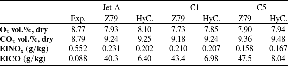
 x=2W=0.28m

 YCO
 YNO
 Z=Zst
 ϕ=0.6


 Open access

