1. Introduction
This paper studies whether voting by city residents of varying incomes has an impact on the level of environmental taxation when residential proximity to a pollution source is taken into consideration. A location model with heterogeneous agents (Brueckner and Selod, Reference Brueckner and Selod2006) is extended to include an environmentally hazardous site, and the degree of damage from pollution is assumed to depend on the distance from this emissions site. The location choice of a resident influences their attitude towards the stringency of environmental policy because the net benefit of public abatement depends on the distance between their residence and the emissions site.
Determining whether the rich or the poor prefer a cleaner environment has long been argued from both a theoretical and empirical point of view. Standard economics tells us that high-income individuals have a stronger preference for a clean environment than those with lower incomes if the environment is a normal good. However, this argument may not explain why, within an electorate, people with high incomes do not necessarily vote for a more stringent environmental policy than those with lower incomes. Kahn and Matsusaka (Reference Kahn and Matsusaka1997), in their empirical studies of voting behavior in California, show that the rich may vote for weaker policies. McAusland (Reference McAusland2003) constructed a model using theoretical viewpoints by assuming that the environment is a necessary good, and found that the rich vote for less stringent policies than the poor. Kahn and Matsusaka (Reference Kahn and Matsusaka1997) indicated that the rich might mitigate environmental problems in private without relying on collective actions. McConnell (Reference McConnell1997) also indicated that the collective demand for environmental improvements is less responsive to income because the propensity for private mitigation, including residential choice, increases with income. Hotte and Winer (Reference Hotte and Winer2012) built a theoretical model by introducing private mitigation. According to their model, the rich may spend more money on their own protection from pollution and do not necessarily require governmental regulation; hence, the demand for a more stringent environmental policy decreases as income levels rise. Their argument is convincing and seems appropriate for environmental issues such as health problems resulting from drinking water contaminated by pesticides or metals, which can be mitigated through the use of water filters if the level of contamination is relatively low. However, averting activities may not be possible or very effective in the case of radioactive waste, chemical water pollution or contaminated land. Private mitigation of outdoor air pollution such as sulfur dioxides or nitrogen oxides may also be impractical, as it is unrealistic for citizens in general to buy professional respirators. In such cases, another option is to reside further away from such point-specific hazardous sites. Gayer et al. (Reference Gayer, Hamilton and Viscusi2000) demonstrated in their empirical analysis that people are willing to pay to reside away from the disamenities associated with Superfund sites.
This type of averting behavior may be dependent on socio-economic status, such as the income level of various residents. From an epidemiological perspective, Brooks and Sethi (Reference Brooks and Sethi1997) constructed an index of exposure to hazardous emissions as a function of the distance to the pollution source. They found that low-income individuals are likely to experience more negative health effects because they tend to reside near the emission sources. In Neidell (Reference Neidell2004), an empirical analysis conducted in California demonstrated that the average level of pollutants is higher for low-income groups. Thus, the negative impact on health is greater for those of lower socio-economic status if they are unable to live in cleaner areas. Studies on potential pollution sources (e.g., hazardous waste landfills) generally demonstrate increased property values per mile away from such facilities (Farber, Reference Farber1998; Boyle and Kiel, Reference Boyle and Kiel2001). As a measure of environmental quality, Brasington and Hite (Reference Brasington and Hite2005) developed a distance-to-hazard index by interpreting the distance between a house and the nearest environmentally hazardous site. They indicated that a greater distance between a house and the nearest environmental hazard is associated with increases in housing prices and residential incomes. This implies that people with high incomes can afford to reside away from pollution sources; however, those with low incomes cannot.
The theory of land use suggests a location choice in geographical space (Fujita, Reference Fujita1989). Brueckner et al. (Reference Brueckner, Thisse and Zenou1999) demonstrated that, if there are amenities that decline with distance from a city center, the rich may live closer to amenities such as libraries and museums. They did not mention negative externality issues such as pollution; however, their analysis implies that the rich may live away from pollution sources and the poor may reside closer to them if the disamenities decrease with distance from polluted areas. From the perspective of public economics, Tiebout (Reference Tiebout1956) indicated that, if both pollution and public abatement are local, the better environment attracts the high-income residents in which the public abatement tax bundles become optimal. This model is different from Tiebout (Reference Tiebout1956) because we analyze the case where private (or local) mitigation is not very effective. While citizens can partially choose their pollution levels through their residential choices, such averting activities may not be sufficient to achieve the optimal level of pollution. In such a case, government regulation is required to control the aggregate pollution in the city.
This study examines whether low-income individuals vote for a more stringent environmental policy than high-income individuals. The analysis suggests that the income level of the median voter is negatively correlated with the equilibrium tax rate, because residents with low incomes live closer to the emissions site and benefit more from pollution abatement. The remainder of this paper is organized as follows. Section 2 provides the basic model for the analysis. Section 3 determines the socially optimal environmental tax rate as well as the tax rate in political equilibrium. Section 4 concludes.
2. Model
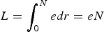
In this study, an amenity-based theory of location (Brueckner and Selod, Reference Brueckner and Selod2006), which examined a transport-system choice under a voting process, is modified to include the negative externality of emissions. The analysis assumes a linear city of unit width and the area of the city is fixed. In this city, N residents consume one unit of land for housing; hence, the length of the city is N. The land is owned by absentee landlords, and the rent earned by land outside the city is assumed to be zero. Residents consume a composite good c produced using a constant-returns technology that employs labor as a single input. L is the aggregate labor input in effective units; thus, the city's output is yL, where y(>0) is the wage per effective labor unit. Each consumer is assumed to offer an effective labor input of e units. The city's aggregate labor input is
 $L = \int_{0}^{N}edr = eN$
; therefore, the aggregate output level is yL=Y=eyN. The model assumes that production does not require any land and there is neither transport cost nor commuting cost for simplicity of analysis. The composite good is assumed to be produced at one edge of the city: the site of production is a single environmentally hazardous site and is a source of emissions such as chemical air pollutants or industrial waste. The distance to this point-specific site is denoted by r. The aggregate level of pollution P is assumed to depend positively on the aggregate emissions Z, which is proportional to the aggregate output such that Z=Y and which depends negatively on public pollution abatement M financed by revenues from emissions taxation.
The government is assumed to levy an emissions tax τ in proportion to the level of emissions,
 $\tau Z = \tau Y = \tau eyN$
. Labor is the only input for production and the labor market is competitive; thus, a consumer with e labor input receives wage from after-tax output, e(1−τ)y.
Because the aggregate pollution is given for voters, the emissions tax rate τ is determined through majority voting. The preferences of the consumers include negative effects from aggregate pollution v(P), where v(P) is an increasing and convex function of pollution (i.e., v
P
>0 and
 $v_{PP} \gt 0$
). However, the degree of exposure to pollution depends on the distance to the emissions site; hence, individuals choose where to reside in the city by taking environmental concerns into consideration. In this model, the degree of exposure to pollution is assumed as a linearly decreasing function of the distance from the emissions site. The strength of the preference for pollution reduction increases with skill level e, i.e.,
 $(\delta - re)v(P)$
, where δ is the parameter for maximum damage at the edge of the city (i.e., at r=0) and the negative externality of pollution requires that δ>re. The assumption is explained further in a model with income heterogeneity that appears in subsection 2.2.
An individual resident maximizes the following utility function:
 $$u(r) = c - (\delta - re) v(P),$$
subject to
 $$c = e(1 - \tau)y - R(r),$$
and
 $$P = Z - M = Y - M,$$
where R(r) is the land rent at location r,
 $M = \phi \tau Y = \phi \tau eyN$
and
 $P = (1 - \phi \tau)eyN$
. ϕ∈[0, 1] is the efficiency index of public abatement. The level of utility is given by substituting (2) into (1):
 $$u(r, \tau) = e(1 - \tau)y - (\delta - re)v(P) - R(r).$$
Before examining the land-market equilibrium, we consider the socially optimal rate of environmental taxation where private ownership of land is not allowed and a social planner decides the level of environmental taxation. The damage costs in this case are given as
 $$v(P)\int_{0}^{N}(\delta - re)dr = v(P)\left[\delta r - {er^{2} \over 2} \right] _{0}^{N} = v(P) N\left(\delta - {eN \over 2} \right).$$
The social optimum is determined by including aggregate land rent Ψ, which is equivalent to the model under public land ownership. The social surplus S(τ) of the entire city is described by the following equation:
 $$S(\tau) = Nu(\tau) + \Psi = N\left\{e(1 - \tau)y - \left(\delta - {eN \over 2} \right) v \lsqb (1 - \phi \tau)eyN \rsqb \right\},$$
where the social surplus is per capita utility times the number of residents with the aggregate land rent. For now, the aggregate land rent Ψ is equal to zero without the land market. The above equation gives the first-order condition for the social optimum as
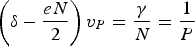
 $$\left(\delta - {eN \over 2}\right) v_{P} = {1 \over \phi} {1 \over N}.$$
This condition indicates that the average marginal damage cost on the left-hand side is equal to the average marginal abatement cost on the right-hand side.
2.1. Land-market equilibrium with absentee land ownership: the homogeneous case
This subsection focuses on the land-market equilibrium in which residents are supposed to have a homogeneous skill. Even in this basic model, the assumption of absentee land ownership makes the equilibrium different from the social optimum because the objective function does not include the aggregate rent of landlords.
At the locational equilibrium, a resident's utility is locationally invariant, whereas c varies with location. If a resident lives closer to the emissions site, the negative effects from pollution increase. However, this impact is exactly offset by an increase in consumption due to rent reduction. Therefore, residents are indifferent to their residential locations. The level of utility given by (3) is equal to the utility at the edge of the city (r=0), that is,
 $$u(\tau) = e(1 - \tau)y - \delta v(P) - R(0).$$
As the level of pollution is given, the land rent at the emissions site is assumed to be equal to zero; consequently, the bid rent at the equilibrium is derived as a function of the distance to the hazard, that is,
 $$R(r) = rev(P)(\geq 0).$$
The slope of the bid-rent function is upward with respect to r for a given aggregate pollution level (i.e.,
 $R^{\prime}(r) \gt 0$
). This is suggested by standard hedonic studies of environmental quality such as Brookshire et al. (Reference Brookshire, Thayer, Schulze and d'Arge1982), provided that environmental quality increases with distance to the emission source (Brasington and Hite, Reference Brasington and Hite2005).
Substituting (4) back into (3) provides the equilibrium utility in the city:
 $$u(\tau) = e(1 - \tau)y - \delta v(P).$$
The equilibrium emissions taxation in the homogeneous case is derived by maximizing the utility function
 $$u(\tau) = e(1 - \tau)y - \delta v \lsqb (1 - \phi \tau) eyN \rsqb ,$$
which generates the first-order condition at the land-market equilibrium P* and its corresponding tax rate τ* in the homogeneous case as
 $$\delta v_{P} = {1 \over \phi} {1 \over N}.$$
Next, the social optimum in the case of homogeneous skill is determined by including aggregate land rent. Aggregate land rent Ψ is derived from (4) as
 $$\Psi = \int_{0}^{N} rev (P)dr = ev (P) \int_{0}^{N} rdr = ev (P) \left. {r^{2}\over 2} \right\vert_{0}^{N} = ev(P) {N^{2} \over 2}.$$
Using (5) and (7), the social surplus can be described as the sum of individual utilities with the aggregate land rent as follows:
 $$S(\tau) = Nu + \Psi = N \left\{e (1 - \tau) y - \left(\delta - {eN \over 2} \right) v \lsqb (1 - \phi \tau) eyN \rsqb \right\}.$$
Maximizing this surplus provides the first-order condition for the social optimal pollution P o and its corresponding tax rate τ o ,
 $$\left(\delta - {eN \over 2} \right)v_{P} = {1 \over \phi} {1 \over N}.$$
Proposition 1
Under the assumption of absentee landownership, the equilibrium tax rate is greater than the optimal rate; hence, the equilibrium pollution reduction exceeds the social optimum.
Proof: The average marginal damage cost in (8) is lower than that in (6); therefore,
 $\tau^{o} \gt \tau^{\ast}$
and P
o
<P* are obtained. □
Proposition 1 is based on the assumption of absentee landownership. The equilibrium level of pollution reduction is determined only by the city residents. However, land owners earn the rent and can consume more; therefore, a land owner may not have to take care of the environment to keep his/her utility constant. If the social surplus, excluding the aggregate land rent, were maximized, the derived pollution reduction at the optimal level would be equal to that at the equilibrium.
2.2. A model with income heterogeneity
This subsection analyzes the case in which consumers have heterogeneous skill values and they choose where to reside in this linear city. Fujita (Reference Fujita1989) suggests that the relative steepness of the bid-rent function of a resident determines where he/she lives in the city. As previously mentioned, several analyses including Brasington and Hite (Reference Brasington and Hite2005) demonstrated that a greater distance to a hazard is associated with an increase in the resident's income. This finding indicates that the absolute value of the marginal rate of substitution between exposure to pollution and composite good consumption (
 $\vert MRS\vert $
) is an increasing function of income since the environment is a normal good. Brueckner et al. (Reference Brueckner, Thisse and Zenou1999) demonstrated that, if the utility function takes the CES form, the elasticity of substitution (ε) should be less than 1 for
 $\vert MRS\vert $
to increase in income, due to the substitution effect between composite good and land consumption. However, if unitary land consumption is assumed, this is not necessarily the case. Consider a maximization problem:
 $\max u[c,d(r)],$
subject to c=ey−R(r), where d(r) is exposure to pollution from a hazardous site, u
d
<0, u
c
>0 and pollution damage decreases as the distance to the emissions site increases, i.e.,
 $d^{\prime}(r) \lt 0$
, following Bellettini and Hubert (Reference Bellettini and Hubert2013). For the locational equilibrium,
 ${\partial u \over \partial r} = 0$
should be satisfied. The first-order condition is
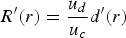 $R^{\prime} (r) = {u_{d} \over u_{c}}d^{\prime}(r)$
. Suppose that individual 2 is richer than individual 1, that is, e
1<e
2. If the poor individual chooses a residence near the pollution source in equilibrium, the difference between the bid-rent slopes at the residential boundary
 $\bar{r}$
for the two income groups must be positive:
 $\Delta \equiv R_{2}^{\prime}(\bar{r}) - R_{1}^{\prime}(\bar{r}) = [v_{d2}(\bar{r}) - v_{d1}(\bar{r})]d^{\prime}(\bar{r}) \gt 0$
, where R
1(r) and R
2(r) are the bid-rent functions for residents with skill levels e
1 and e
2, respectively. In the case of a CES utility function,
 $\vert MRS\vert $
is an increasing function of income as long as ε>0.Footnote
1
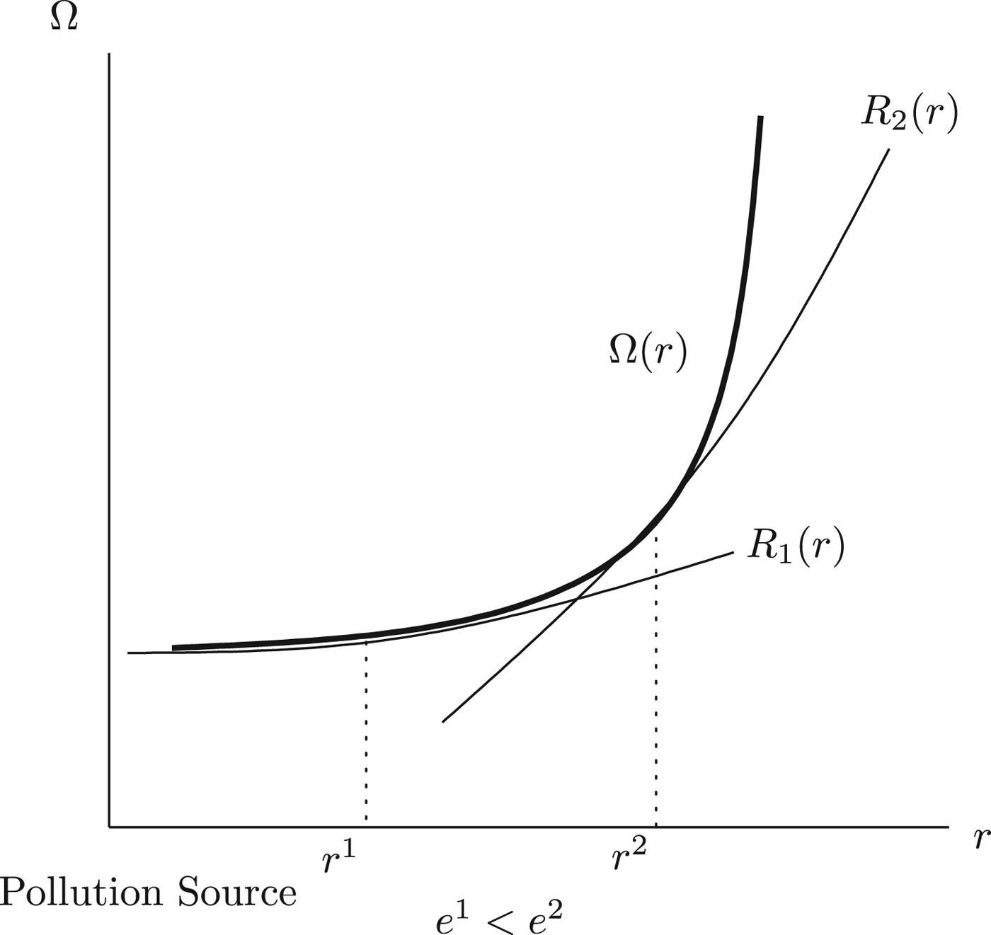
Let Ω(r) be the market-rent function that is exogenously determined. Following Brueckner and Selod (Reference Brueckner and Selod2006), the slope of the bid-rent function is supposed to be linear in income and the degree of exposure to pollution is a linearly decreasing function of the distance from the emissions site, that is,
 $d(r) = \delta - re$
. Under this setting, the residential pattern as determined in equilibrium is shown in figure 1.
Bid-rent functions and residential locations

This figure illustrates the case in which skill heterogeneity is introduced.Footnote
2
If e
1<e
2, r
1<r
2 is obtained because
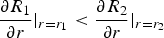 ${\partial R_1 \over \partial r} \vert_{r =r_1} \lt {\partial R_2 \over \partial r} \vert_{r = r_2}$
. This inequality indicates that if aggregate pollution is given, residents with high incomes prefer a location further from the emission source. This residential pattern is suggested by several empirical studies such as Brooks and Sethi (Reference Brooks and Sethi1997) and Neidell (Reference Neidell2004).
In this case, the utility levels vary with e, that is, u(e), so that the resident with a particular e offers the highest bid for the land at r(e). The skill distribution is given by the interval
 $\lsqb \underline{e}, \overline{e} \rsqb $
, and g(e) and G(e) are defined as the density and the cumulative distribution functions, respectively. If the distribution of residents is such that the distance increases with the skill level, the residential distance of a consumer with skill e, that is, r(e), is given by
 $$r(e) = N \int_{\underline{e}}^{e} g (w) dw = NG(e).$$
The equation shows that r(e) is equal to the number of people with skills less than e because the distance to the hazardous site is equivalent to the number of people with skills less than e under the assumption of unitary land consumption. Assuming that the aggregate pollution is constant, the bid-rent function is derived from (3) as
 $$R[r(e),e] = e(1 - \tau)y - [\delta - r(e)e] v (P) - u(e).$$
This equation implies that, for a given e, the slope of the rent function with respect to r is positive and steeper for a larger e. If a particular individual with a high e is the highest bidder at a location, that location must have a high r value. That is, the resident with the lowest skill level lives closest to the emissions site, and the individual with the highest skill level resides at the other side of the city's edge.Footnote 3
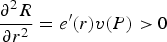
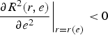
Following Brueckner and Selod (Reference Brueckner and Selod2006), for the residential pattern given by (9) to appear at the equilibrium, an individual with skill level e must bid more for the land at r(e) than anyone else. That is, holding r fixed at r(e) in equation (10), the maximum of
 $R\lsqb r(e),e^{\prime} \rsqb $
must be reached at e′=e, that is,
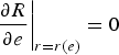
 $$\left. {\partial R(r,e) \over \partial e} \right\vert_{r = r(e)} = (1 - \tau )y + r(e)v(P) - u^{\prime}(e) = 0.$$
Substituting (9) into this equation provides the following differential equation:
 $$u^{\prime}(e) = (1 - \tau)y + v(P) N \int_{\underline{e}}^{e}g(w)dw.$$
Integrating this differential equation yields the utility function
 $$u(e) = e(1 - \tau)y + v(P) N \int_{\underline{e}}^{e}G(w)dw + A,$$
where A is a constant. By substituting (11) into (10), the bid-rent function can be rewritten as
 $$R(r,e) = -(\delta - re) v (P) - v (P) N \int_{\underline{e}}^{e}G(w)dw - A.$$
The land rent at the emissions site where the least skilled individual resides is assumed to be zero, that is,
 $R(0,\underline{e}) = 0$
. This assumption determines the constant term
 $A = - \delta v(P)$
. Assuming that the aggregate pollution is given, if the constant term is substituted back into (12), the bid-rent function with income heterogeneityFootnote
4
is provided as
 $$R(r,e) = \lsqb re - N \Gamma (e) \rsqb v(P),$$
where
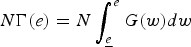 $N\Gamma(e) = N\int_{\underline{e}}^{e}G(w)dw$
. This is the sum of distances of all the residents with skills less than e from the emissions site to their residences. Substituting the constant
 $A=-\delta v(P)$
into (11) generates the following utility function with heterogeneityFootnote
5
:
 $$u(e, \tau) = e(1 - \tau)y - \lsqb \delta - N \Gamma (e) \rsqb v(P).$$
3. Social optimum, political equilibrium and environmental taxation rates
In this section, the socially optimal level of emissions taxation is compared to the tax level in the political equilibrium. First, the socially optimal level of emissions taxation is determined by maximizing the surplus. Next, the preferred level of emissions tax in a democratic society is resolved through majority voting. Finally, the effect of an increase in skill level on the equilibrium taxation is investigated.
3.1. Social optimum
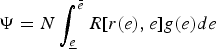
The optimum in the case of income heterogeneity with the land market is examined. The aggregate land rent
 $\Psi = N \int_{\underline{e}}^{\bar{e}} R[r(e),e]g(e)de$
is derived from (13) as
 $$\Psi = Nv(P) \left[ NJ - N \int_{\underline{e}}^{\bar{e}} \Gamma (e) g(e) de \right],$$
where
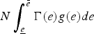 $N\int_{\underline{e}}^{\bar{e}}\Gamma(e)g(e)de$
is the expected sum of distances of all the residents and
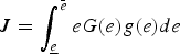 $J = \int_{\underline{e}}^{\bar{e}} eG(e) g(e) de$
. Similarly to the previous section, the surplus in the heterogeneous case is aggregate utilities with the aggregate land rent, that is,
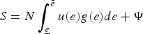 $S = N\int_{\underline{e}}^{\bar{e}} u(e) g(e) de + \Psi$
. The optimum is determined by maximizing the following surplus:
 $$S(\tau) = N\lsqb (1 - \tau)e_{m}y - \lpar \delta - NJ \rpar \rsqb v\lsqb (1-\phi \tau) ye_{m} N \rsqb ,$$
where e m is the skill level of the mean voter. The first-order condition for the optimum is generated as
 $$\lpar \delta - NJ \rpar v_{P} = {1 \over \phi} {1 \over N},$$
which is equivalent to the optimal condition without the land market. Because the aggregate land rent is at least zero by assumption (i.e.,
 $\Psi (e) \geq 0$
), the following inequality is obtained:
 $$J = \int_{\underline{e}}^{\bar{e}} eG(e) g(e) de \geq \int_{\underline{e}}^{\bar{e} } \Gamma (e) g(e) de.$$
This relationship is used in the next subsection.
3.2. Political equilibrium
The equilibrium tax rate is determined through majority voting by maximizing the utility derived from (14) as
 $$u(e,\tau) = e(1 - \tau) y - \lsqb \delta - N \Gamma (e) \rsqb v \lsqb (1 - \phi \tau) e_{m} yN \rsqb ,$$
with respect to the rate of emissions taxation τ. The following first-order condition for the voting equilibrium is obtainedFootnote 6 :
 $$\lsqb \delta - N \Gamma (\hat{e}) \rsqb v_{P} = {1 \over \phi} {\hat{e} \over e_{m}N},$$
which provides the equilibrium pollution P̂ and its corresponding tax rate τ̂ determined by the median voter, where
 $\widehat{e}$
is the skill level of the median voter.
Now, the voting equilibrium determined by the median voter is compared with the equilibrium pollution and the tax rate chosen by the mean voter, P
m
and τ
m
, respectively and the social optimum (15). Define the (average) marginal abatement cost (MAC) on the right-hand side of equation (17) at the equilibrium. This is equal to the socially optimal level
 ${1 \over \phi} {1 \over N}$
on the right-hand side of the equation (15) if ê=e
m
. However, as Becker and Tomes (Reference Becker and Tomes1979) mentioned, actual income distributions tend to be skewed to the right. If we assume that the distribution of skills is skewed in the direction of high skills, the skill level of the median voter is less than that of the mean voter, that is,
 $\widehat{e} \lt e_{m}$
. Consequently, MAC in the voting equilibrium described on the right-hand side of equation (17) is lower than MAC at the optimum. This is because the abatement cost share is proportional to the level of income such that pollution reduction is relatively less expensive for residents with low incomes.
Next, let the (average) marginal damage cost function be
 $MDC(e) = \lsqb \delta - N \Gamma (e) \rsqb v_{P}(\gt 0)$
. Γ(e) is a convex function with respect to e as
 $\Gamma^{\prime}(e) = G (e) \gt 0$
and
 $\Gamma^{\prime \prime}(e) = G^{\prime}(e) = g(e) \gt 0$
; thus, the marginal damage cost function is a concave function with respect to the skill level e, as shown by
 $$\eqalign{{\partial {MDC}(e) \over \partial e} & =-N\Gamma^{\prime}(e)v_{P} = - {NG}(e)v_{P} \lt 0,\cr {\partial^{2} {MDC}(e) \over \partial e^{2}} & = - {NG}^{\prime}(e)v_{P} = - {Ng}(e)v_{P} \lt 0.}$$
Following Jensen's inequality for a concave function, we have
 $$\left[\delta - N \int_{\underline{e}}^{\bar{e}} \Gamma (e) g(e) de \right] v_{p} \lt \lsqb \delta - N \Gamma (e_{m}) \rsqb v_{P}.$$
The inequality (18) demonstrates that the city's average marginal damage cost is less than the damage cost of the mean voter. This inequality, accompanied by (16), also indicates that
 $$J \ge \int_{\underline{e}}^{\bar{e}} \Gamma (e) g(e) de \gt \Gamma (e_{m}) \gt \Gamma (\hat{e}),$$
where ê<e m .
Proposition 2
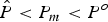
In case of income heterogeneity, the equilibrium tax rate determined by the median voter is larger than that of the mean voter, both of which are larger than the optimum. Therefore, pollution at the equilibrium determined by the median voter is smaller than the pollution level chosen by the mean voter, both of which are smaller than the optimum.
Proof: With regard to MAC, MAC in the voting equilibrium is lower than MAC at the optimum. Next, with respect to MDC, the inequalities in (19) demonstrate that
 $NJ \geq N \int_{\underline{e}}^{\bar{e}} \Gamma (e) g(e) de \gt N \Gamma (e_{m}) \gt N \Gamma (\hat{e})$
, i.e., the median voter's distance from the hazardous site is shorter than that of the mean, and the mean voter's distance from this site is shorter than the optimal distance. The comparison between (17) and (15) associated with these inequalities shows that MDC of the median voter is larger than MDC of the mean resident, which is larger than MDC at the optimum. Combining these two effects with the convexity of the function v(P) with regard to P, we obtain
 $\hat{\tau} \gt \tau_{m} \gt \tau^{o}$
and
 $\hat {P} \lt P_{m} \lt P^{o}$
. □
Please note that, in proposition 2, while the disparity between
 $N\Gamma (e_{m})$
and
 $N\Gamma (\hat{e})$
stems from the skewness of the skill distribution, the divergence between
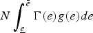 $N \int_{\underline{e}}^{\bar{e}} \Gamma (e) g(e) de$
and
 $N \Gamma (e_{m})$
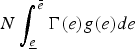
results from the concavity of the MDC function with regard to e. In addition, the difference between NJ and
 $N\int_{\underline{e}}^{\bar{e}} \Gamma (e) g (e) de$
is derived from the existence of the aggregate rent Ψ.
The above argument indicates that the equilibrium rate of emissions tax exceeds the optimal taxation rate. Now, we will find what would happen to the equilibrium emissions tax level if the skill level of the median voter were to increase.Footnote
7
From the equilibrium condition (17), the marginal net benefit from emissions taxation,
 $F(\hat{e},\tau)$
, can be defined as
 $$F (\hat{e}, \tau) \equiv {\partial u \over \partial \tau} = \lsqb \delta - N \Gamma (\hat{e}) \rsqb v_{P} [(1 - \phi \tau) e_{m} yN] - {1 \over \phi} {\hat{e} \over e_{m}N}.$$
Partially differentiate
 $F(\hat{e},\tau)$
with respect to ê to obtain
 $${\partial F(\hat{e},\tau) \over \partial \hat{e}} \equiv F_{\hat{e}} = - \left[ NG (\hat{e}) v_{P} + {1 \over \phi e_{m}N} \right] (\lt 0).$$
This partial differential equation demonstrates that the marginal net benefit of taxation decreases as income rises. This is because the damage to highly skilled individuals is less than the damage to less skilled ones (the first term on the right-hand side), and because tax payments increase with income (the second term on the right-hand side). Partially differentiate
 $F(\hat {e},\tau)$
with regard to τ to obtain
 $${\partial F(\hat{e},\tau) \over \partial\tau} \equiv F_{\tau} = - \phi e_{m} yN \lsqb \delta - N \Gamma (\hat{e}) \rsqb v_{PP} (\lt 0).$$
Totally differentiate
 $F(\hat{e},\tau)$
to yield
 $${d\tau \over d \hat{e}} = - {F_{\hat{e}} \over F_{\tau}} \lt 0.$$
This inequality displays that in the political equilibrium, if the skill level of the median voter increases, the equilibrium level of emissions taxation declines. In this setting, the abatement cost share is proportional to the level of income; furthermore, the benefits from pollution reduction are disproportional to skill levels. Therefore, imposing an emissions tax places a disproportionate welfare burden on skilled residents.
4. Conclusion
This study has investigated the political economy of an environmental policy with residential locations. A location model with heterogeneous agents has been modified to include the negative externality of emissions. In the analysis, a single environmentally hazardous site is assumed to exist at the edge of a linear city. An emissions tax is levied and the tax rate is determined through majority voting. The degree of damage caused by pollution depends on the distance from the emissions site; therefore, the distance to the environmentally hazardous site is positively associated with housing prices. Voters with low incomes are likely to live near the hazardous site, and are damaged more than the rich by the aggregate pollution. Consequently, residents with low incomes vote for a higher rate of pollution tax because their benefits in reducing aggregate pollution are higher than those of average residents.
This analysis shows that a reduction in the median voter's income leads to a higher equilibrium tax rate. While Hotte and Winer (Reference Hotte and Winer2012) introduced private mitigation, this study explores spatial aspects to address the issue. The analysis focuses on a case in which averting behavior does not effectively improve the problem and, hence, a possible solution is to reside away from the point-specific hazardous site.
The quality of the environment is one of the important factors that influence the value of housing. Areas with good environmental quality can charge higher rents, and therefore only the rich can afford to live in these areas. The widening income gap between the rich and the poor accelerates the geographical separation of their residential areas. This trend is now widespread in most developed countries. The analysis implies that such a circumstance may lead to the equilibrium pollution reduction being determined through a majority voting that would be different from the optimum.
This argument has several limitations. For example, policy packages comprising income transfers to narrow the income gap between the rich and the poor might be effective in reducing the difference between the optimum and the equilibrium. In addition, the location of a hazardous site is not endogenously determined. These factors require further examination.