1. INTRODUCTION
Whistler waves are important not only in space plasma due to wave particle interactions, but also in laboratory plasmas as helicons for efficient plasma production as well as acceleration (Karpman & Washimi, Reference Karpman and Washimi1977; Shukla, Reference Shukla1978; Spatschek et al., Reference Spatschek, Shukla, Yu and Karpman1979; Shukla & Stenflo, Reference Shukla and Stenflo1984; Rao, Reference Rao1988; Karpman et al., Reference Karpman, Hansen, Huld, Lynov, Pecseli and Rasmussen1990; Zhao et al., Reference Zhao, Lu and Wu2010). Large amplitude whistlers propagating in a magnetized plasma can initiate a great variety of non-linear effects, modulation instability (Zhao et al., Reference Zhao, Lu and Wu2010), and the subsequent soliton formation (Karpman & Washimi, Reference Karpman and Washimi1977; Shukla, Reference Shukla1978; Shukla & Stenflo, Reference Shukla and Stenflo1984). Whistlers also contribute to fast magnetic reconnection and plasma dynamics in two beam laser–solid density plasma interaction experiments. Whistler can make electrons go faster to high energies. Chen et al. (Reference Chen, Tajima and Takahashi2002) showed clearly that particles may go faster by plasma magneto waves, plentiful in astrophysical settings. Particle-in cell simulations have shown good results for celestial acceleration (Chen et al., Reference Chen, Chang, Lin, Noble and Sydora2009). Lower hybrid waves have been used to maintain runaway electrons in a tokamak to give the toroidal current. Recent experiments have observed MeV electrons during lower hybrid heating/current drive in the tokamak.
Lately, significant progress has been made in the field of plasma-based accelerators for attaining high electron energies (Tajima & Dawson, Reference Tajima and Dawson1979; Brodin & Lundberg, Reference Brodin and Lundberg1998; Joshi, Reference Joshi2007; Schlenvoigt et al., Reference Schlenvoigt, Haupt, Debus, Budde, Jackel, Protenhauer, Schwoerer, Rohwer, Gallacher, Brunetti, Shank, Wiggins and Jaroszynski2008; Caldwell et al., Reference Caldwell, Lotov, Pukho and Simon2009; Shukla, Reference Shukla2009). The advent of high-power lasers has led to a scheme that can produce large-phase velocity plasma waves and the latter can accelerate electron to hundreds of MeV energy. Work on acceleration by ponderomotive force of the laser pulse has been pursued vigorously and electron acceleration approaching GeV energy is being achieved (Tsakiris et al., Reference Tsakiris, Gahn and Tripathi2000; Tochitsky et al., Reference Tochitsky, Narang, Filip, Musumeci, Clayton, Yoder, Marsh, Rosenzweig, Pellegrini and Joshi2004; Liu & Tripathi, Reference Liu and Tripathi2005; Sazegari et al., Reference Sazegari, Mirzaie and Shokri2006; Zhidkov et al., Reference Zhidkov, Fujii and Nemoto2008; Kalmykov et al., Reference Kalmykov, Yi and Shvets2009). The electron energies are far in excess of ponderomotive potential energy, and the acceleration is a consequence of direct exchange of energy between electron and laser via betatron resonance. Gahn et al. (Reference Gahn, Tsakiris, Pukhov, Meyer-Ter-Vehn, Pretzler, Thirolf, Habs and Witte1999) reported generation of multi-MeV electrons by direct laser acceleration in high-density plasma channels. Tsakiris et al. (Reference Tsakiris, Gahn and Tripathi2000) developed a theoretical laser model of direct acceleration. Microwave and radio waves provide another frequency regime for particle acceleration.
The low-temperature dense electron plasmas are degenerate and obey Fermi–Dirac statistics. The high-density, low-temperature quantum Fermi plasma is significantly different from the low-density, high-temperature ‘classical plasma’ obeying the Maxwell–Boltzmann distribution. The study of highly dense quantum plasmas becomes important, when the de Broglie thermal wavelength associated with the charged particle, that is,
 ${\rm \lambda} _{\rm B} = \hbar /(2 {\rm \pi} mk_{\rm B}T)$
approaches the electron Fermi wavelength λFe and exceeds the electron Debye radius
 ${\rm \lambda} _{{\rm De}}\,({\rm viz}.,{\rm \lambda} _{\rm B} \sim {\rm \lambda} _{{\rm Fe}} \gt {\rm \lambda} _{{\rm De}})$
. Furthermore, the quantum effects associated with the strong density correlation start playing a significant role when λB becomes of the same order or larger than the average interparticle distance
 $(\sim n_0^{ - {1 / 3}})$
, that is,
 $n_0{\rm \lambda} _{\rm B}^3 \ge 1$
hold in the degenerate plasma. However, the other condition for degeneracy is that the Fermi temperature (T
F), which is related to the equilibrium density (n
0) of the charged particles must be greater than the thermal temperature (T) of the system (Gardner & Ringhofer, Reference Gardner and Ringhofer1996; Haas et al., Reference Haas, Garcia, Goedert and Manfredi2003; Shukla & Eliassion, Reference Shukla and Eliassion2010; Shukla & Akbari-Maghananghi, Reference Shukla and Akbari-Maghananghi2012).
In the present work, we focus on the recently developed quantum hydrodynamic (QHD) model (Shukla & Eliasson, Reference Shukla and Eliasson2006). The QHD model consists of a set of equations describing the transport of charge density, momentum (including the Bohm potential), and energy in a charge particle system interacting through a self-consistent electrostatic potential (Kumar & Tewari, Reference Kumar and Tewari2012). In particular, the two main limitations of the QHD model (Crouseilles et al., Reference Crouseilles, Hervieux and Manfredi2008) are that: (a) quantum effects are included only to second order in the Planck's constant and (b) wavelengths shorter than the Thomas–Fermi screening length λF are not treated properly. Here (λF = νF/ωpe), where νF is the Fermi speed and ωpe is the plasmon frequency. The latter restriction is analogous to the well-known limitation for classical fluid models, which are valid for wavelengths longer than the Debye length (i.e., the typical screening length in a classical plasma). The advantages of the QHD model over kinetic descriptions are its numerical efficiency, the direct use of the macroscopic variables of interest such as momentum and energy and the easy way the boundary conditions are implemented.
For metallic structures, the electron density is very high
 $(n \sim 10^{28}\;{\rm m}^{ - 3})$
, yielding a Fermi temperature
 $(T_{\rm F}\sim 5 \ \times 10^4\;{\rm K})$
. Thus, for most practical purposes, metallic structures can be thought of as operating effectively at zero electron temperature (Crouseilles et al., Reference Crouseilles, Hervieux and Manfredi2008). Electromagnetic pulses with intensity of the order of 1018 W cm−2 are able to break the internal Coulomb field of the atoms in a solid. Thin films irradiated with such intense sources of microwave radiation can expel electrons with extremely high energies (10–100 MeV). In the X-ray domain, lasers with intensity of 1014 W cm−2 and energy about 1 keV are currently applied to different areas (Morandi et al., Reference Morandi, Zamanian, Manfredi and Hervieux2014).
In this paper, we analytically examine electron acceleration by the ponderomotive force associated with a right circularly polarized Gaussian whistler pulse in a magnetized quantum plasma. Initially, the electrons have speeds lower than the group velocity of the whistler pulse, and the ponderomotive force pushes electrons ahead of the pulse. The group velocity of the whistler pulse is significantly less than the speed of light, and hence electrons can resonantly interact with the pulse. One expects the saturation to occur when the electron velocity exceeds the pulse group velocity and the electron outruns the whistler pulse. The theoretical formalism has been explained in Section 2. Section 3 is devoted to conclusions.
2. ACCELERATION
We consider the propagation of a right circularly polarized whistler pulse in high-density quantum plasma in the direction of static magnetic field
 $B_{\rm s}\hat z$
. The electric and magnetic fields of the whistler are (Singh & Sharma, Reference Singh and Sharma2010).
 $$\vec E = (\hat x + i\hat y)A_{\rm 0}(z - v_{\rm g}t)\exp \left[ { - i({\rm \omega} t - kz)} \right],$$
 $$\vec B = - \left[ {\displaystyle{1 \over {\rm \omega}} \left( {1 - \displaystyle{{v_{\rm g}k} \over {\rm \omega}}} \right)\displaystyle{{\partial A_{\rm o}} \over {\partial z}} + \displaystyle{{ik} \over {\rm \omega}} A_{\rm 0}} \right](\hat x + i\hat y),$$
where A 0 for a Gaussian pulse is given by
 $$A_0^2 = A_{00}^2 \exp \left[- {(t - z/v_{\rm g}})^2 / {\rm \tau}^{2} \right],$$
where,
 $k = ( {\rm \omega} /c)[(1 - {\rm \omega} _{\rm p}^2 )/{\rm \omega} ({\rm \omega} - {\rm \omega} _{\rm c})]^{1/2}$
, νg = ∂ω/∂k is the pulse group velocity, τ is the pulse duration,
 $ {\rm \omega} _{\rm p}^2 = (4 {\rm \pi} n_{\rm 0}e^2/m)$
is the electron plasma frequency, ωc = eB
s/mc is the electron cyclotron frequency, m is the rest mass of electron, c is the velocity of light in vaccum.
The QHD equations governing the motion of electron in the presence of laser field and the static magnetic field is given (Kumar & Tewari, Reference Kumar and Tewari2012)
 $$\displaystyle{{d\vec p} \over {dt}} = - e\vec E - \displaystyle{e \over c}(\vec v \times \vec B) - \displaystyle{{{\rm \nu} _{\rm F}^2} \over {3n_{\rm 0}^2}} \displaystyle{{\vec \nabla n^3} \over n} + \displaystyle{{\hbar ^2} \over {2m}}\vec \nabla \left( {\displaystyle{1 \over {\sqrt n}} {\vec \nabla} ^2\sqrt n} \right),$$
 $$\displaystyle{{\partial n} \over {\partial t}} + \vec \nabla . (n\vec v) = 0,$$
where n( = n
0 + n
(1)) is the electron density and
 $\hbar $
is the Planck's constant divided by 2π,
 ${\rm \nu} _{\rm F}( = (\hbar /m)(3 {\rm \pi} ^2n)^{{1 / 3}})$
is the Fermi velocity. The third term on the right-hand side of Eq. (4) denotes the Fermi electron pressure
 $( = m{\rm \nu} _{\rm F}^2 n^3/3n_0^3 )$
. The fourth term is the quantum Bohm force and is due to the quantum corrections in the density fluctuation. The classical equation may be recovered in the limit of
 $\hbar = 0.$
The ponderomotive force of the high-frequency laser pulse drives longitudinal waves with a frequency much smaller than ω, but fast enough for the dynamics to take place in the electron time scale. The ions form a neutralizing background in dense plasma. A correct relativistic treatment of quantum effects should rely on the moments of a relativistic wigner function. Simultaneous solution of Eqs. (4) and (5) gives the electron velocity and electron density as
 $$\vec v = \displaystyle{{e {\rm \omega} \vec E} \over {mi[({\rm \nu} _{\rm F}^2 + ({\hbar}^2/4m^2)k^2)k^2 - {\rm \omega} ( {\rm \omega} - {\rm \omega} _{\rm c})]}},$$
 $$n = i\displaystyle{{en_0k\vec E} \over {[({\rm \nu} _{\rm F}^2 + ({\hbar ^2}/4m^2)k^2)n_0k^2 - m {\rm \omega} ( {\rm \omega} - {\rm \omega} _{\rm c})]}}.$$
Equation (6) represents the oscillatory motion imparted by the whistler pulse to the plasma electron.
To evaluate the ponderomotive force in the next order, one must remember that
 $\vec v$
and
 $\vec B$
in our representations are complex; however, actual
 $\vec v$
and
 $\vec B$
, and their real parts are implied in ponderomotive force
 $(\vec F_{\rm P})$
. We may use the complex number identity
 ${\mathop{\rm Re}\nolimits} \vec A \times {\mathop{\rm Re}\nolimits} \vec B = (1/2){\mathop{\rm Re}\nolimits} (\vec A \times \vec B + \vec A \times \vec B^*)$
to simplify it, where * refers to the complex conjugate. The ponderomotive force on the electron due to the whistler pulse is thus
 $$\vec F_{\rm P} = - \left( \displaystyle{{m}\over{2}} \right) (\vec v . \vec \nabla )\vec {v}^{\,\,*} - \left( \displaystyle{{e} \over{2}} \right)(\vec v \times \vec B^*).$$
Assuming the magnetic field to vary as
 $\vec B = be^{ - i( {\rm \omega} t - kz)}$
, we get
 $$\displaystyle{{\partial \vec B} \over {\partial t}} = \left( {\displaystyle{{\partial \vec b} \over {\partial t}} - i {\rm \omega} \vec b} \right)e^{ - i( {\rm \omega} t - kz)}$$
and
 $$\vec b = - \displaystyle{1 \over {\rm \omega}} \left( {\displaystyle{{\partial A_0} \over {\partial z}} + ikA_0} \right)(\hat x + i\hat y) - \displaystyle{k \over { {\rm \omega} ^2}}\displaystyle{{\partial A_0} \over {\partial t}}(\hat x + i\hat y).$$
For ∂/∂t = −(∂/∂z)νg, the above equation reduces to
 $$\vec b = - \left[ {\displaystyle{1 \over {\rm \omega}} \left( {1 - \displaystyle{{{\rm \nu} _{\rm g}k} \over {\rm \omega}}} \right)\displaystyle{{\partial A_0} \over {\partial z}} - \displaystyle{{ik} \over {\rm \omega}} A_0} \right](\hat x + i\hat y),$$
where
 $$\left( {1 - \displaystyle{{{\rm \nu} _{\rm g}k} \over {\rm \omega}}} \right) = \displaystyle{{ {\rm \omega} _{\rm P}^2 (2 {\rm \omega} - {\rm \omega} _{\rm c})} \over {2 {\rm \omega} {( {\rm \omega} - {\rm \omega} _{\rm c})}^2(1 + (( {\rm \omega} _{\rm P}^{\rm 2} {\rm \omega} _{\rm c}/ {\rm \omega} )/{\rm 2}{( {\rm \omega} - {\rm \omega} _{\rm c})}^{\rm 2}))}}$$
and
 $${{{\rm \nu} _{\rm g}} \over c} = 1 - \displaystyle{{ {\rm \omega} _{\rm P}^2 / {\rm \omega} ^{2\,}/(2 - {\rm \omega} _{\rm c}/ {\rm \omega} )} \over {2{(1 - {\rm \omega} _{\rm c}/ {\rm \omega} )}^2(1 + ({\rm (} {\rm \omega} _{\rm P}^2 / {\rm \omega} ^2)/( {\rm \omega} _{\rm c}/ {\rm \omega} ))/(2{(1 - {\rm \omega} _{\rm c}/ {\rm \omega} )}^2)}}.$$
The above equation shows that there occurs a cyclotron resonance at ω = ωc, and the group velocity of the whistler pulse vanishes at the cyclotron resonance. Substituting Eq. (11) into (9), we get
 $$\vec B = - \left[ {\displaystyle{1 \over {\rm \omega}} \left( {1 - \displaystyle{{{\rm \nu} _{\rm g}k} \over {\rm \omega}}} \right)\displaystyle{{\partial A_0} \over {\partial z}} - \displaystyle{{ik} \over {\rm \omega}} A_0} \right](\hat x + i\hat y)e^{ - i\left( { {\rm \omega} t - kz} \right)}.$$
Substitution of relevant quantities in Eq. (8) gives the parallel component of the ponderomotive force (with respect to static magnetic field)
 $$F_{{\rm p}z} = - \displaystyle{{e^2} \over {2m\left[ {({\rm \nu} _{\rm F}^2 + ({\hbar ^2}/4m^2)k^2)k^2 - {\rm \omega} ( {\rm \omega} - {\rm \omega} _{\rm c})} \right]}}\left( {1 - \displaystyle{{{\rm \nu} _{\rm g}k} \over {\rm \omega}}} \right)\displaystyle{{\partial A_0^2} \over {\partial z}},$$
which may be further solved to yield
 $$\eqalign{ F_{{\rm p}z} = & - \displaystyle{{e^2} \over {2m\left[ {({\rm \nu} _{\rm F}^2 + ({\hbar ^2}/4m^2)k^2)k^2 - {\rm \omega} ({\rm \omega} - {\rm \omega} _{\rm c})} \right]}} \cr & \times \displaystyle{{{\rm \omega} _{\rm p}^2 (2 {\rm \omega} - {\rm \omega} _{\rm c})} \over {2 {\rm \omega} {( {\rm \omega} - {\rm \omega} _{\rm c})}^2(1 + ({{ {\rm \omega} _{\rm p}^{\rm 2} {\rm \omega} _{\rm c}} / {\rm \omega}} )/(2{( {\rm \omega} - {\rm \omega} _{\rm c})}^2))}}\displaystyle{{\partial A_0^2} \over {\partial z}}.}$$
From the above equation, it is evident that the ponderomotive force F pz reverses its direction at ω = ωc/2. For ω>ωc/2, the front of the whistler pulse exerts a longitudinal force on the electron and there is a net energy gain by the electrons. The equation of motion for an electron in the presence of the ponderomotive force is
 $$\eqalign{\displaystyle{{d^2z} \over {dt^2}} = & - \displaystyle{{e^2} \over {2m^2[(\nu _{\rm F}^{\rm 2} + (\hbar ^2}/4m^2)k^2)k^2 - {\rm \omega }({\rm \omega } - {\rm \omega }_{\rm c})]} \cr& \times \displaystyle{{{\rm \omega }_2^2 (2{\rm \omega } - {\rm \omega }_{\rm c})} \over {2{\rm \omega }{({\rm \omega } - {\rm \omega }_{\rm c})}^2(1 + (({\rm \omega }_{\rm p}^{\rm 2} {\rm \omega }_{\rm c}/{\rm \omega })/2{({\rm \omega } - {\rm \omega }_{\rm c})}^2))}} \cr &\times \displaystyle{{2A_0^2 } \over {\nu _{\rm g}{\rm \tau }^2}}\left( {t - \displaystyle{z \over {\nu _{\rm g}}}} \right)\exp [ - (t - z/\nu _{\rm g})^2/\tau ^2].}$$
Defining ((z − νg t)/νg t) = ξ; dz/dt = νgτ(dξ/dt) + νg, Eq. (17) can be expressed as
 $$\displaystyle{{d^2{\rm \xi}} \over {dt^2}} = \Omega {\rm \xi} e^{ - {\rm \xi} ^2},$$
where
 $$\eqalign{\Omega =\, & \displaystyle{{a_0^2} \over {\left[ {({\rm \nu} _{\rm F}^2 + ({\hbar ^2}/4m^2)k^2)k^2 - {\rm \omega} ({\rm \omega} - {\rm \omega} _{\rm c})} \right]}} \cr &\times \displaystyle{{ {\rm \omega} _{\rm p}^2 (2 {\rm \omega} - {\rm \omega} _{\rm c})} \over {2( {\rm \omega} - {\rm \omega} _{\rm c})\left( {1 + (( {\rm \omega} _{\rm p}^2 {\rm \omega} _{\rm c}/ {\rm \omega} )/(2{( {\rm \omega} - {\rm \omega} _{\rm c})}^2))} \right)}}.} $$
Multiplying both sides of Eq. (18) by 2(dξ/dt) and integrating we get,
 $$\left( {\displaystyle{{d{\rm \xi}} \over {dt}}} \right)^2 = - \Omega e^{ - {\rm \xi} ^2} + c_1,$$
where c 1 is the constant of integration. Using (18), we get
 $$(\nu _z - \nu _{\rm g})^2 = - \Omega e^{ - {((t - z)/\nu _{\rm g})}^2/{\rm \tau }^{\rm 2}} + c_1.$$
At t = −∞, z = 0, and ν z = ν0,
so we get c 1 = (ν z − ν0)2.
At t = ∞, implying
 $$({\rm \nu} _z - {\rm \nu} _{\rm g})^2 = ({\rm \nu} _{\rm g} - {\rm \nu} _{\rm 0})^2,$$
 ${\rm \nu} _z = {\rm \nu} _{\rm g} \pm \sqrt {{({\rm \nu} _{\rm g} - {\rm \nu} _0)}^2} = 2{\rm \nu} _{\rm g} - {\rm \nu }_0$
, when the wave amplitude is large = ν0 when the wave amplitude is small.
It is obvious that the electron with small ν0 (small positive initial velocity) gains less velocity (energy). A counter moving electron will gain larger velocity.
Now, we calculate the normalized threshold whistler amplitude for which ν z = ν0 at ξ = 0, that is, the electron velocity is equal to the group velocity of the whistler pulse. Under these conditions, Eq. (19) reduces to
 $$({\rm \nu} _z - {\rm \nu} _0)^2 - \Omega = 0$$
giving
 $$\eqalign{a_0^2 =\,\,& ({\rm \nu} _{\rm g} - {\rm \nu} _0)^2\left( {\left( {{\rm \nu} _{\rm F}^2 + \displaystyle{{\hbar ^2} \over {4m^2}}k^2} \right)k^2 - {\rm \omega} ( {\rm \omega} - {\rm \omega} _{\rm c})} \right) \cr & \times\, \displaystyle{{2( {\rm \omega} - {\rm \omega} _{\rm c})\left( {1 + (( {\rm \omega} _{\rm p}^{\rm 2} {\rm \omega} _{\rm c}/ {\rm \omega} )/2{( {\rm \omega} - {\rm \omega} _{\rm c})}^2)} \right)} \over { {\rm \omega} _{\rm p}^2 (2 {\rm \omega} - {\rm \omega} _{\rm c})}}.}$$
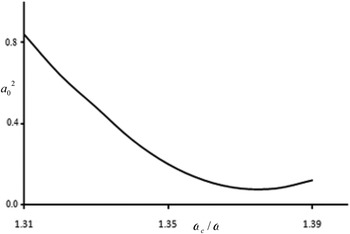
Figure 1 shows the variation of normalized whistler amplitude
 $a_0^2 $
with ωc/ω for
 $ {\rm \omega} _{\rm p}^2 / {\rm \omega} ^{\rm 2} = 0.3$
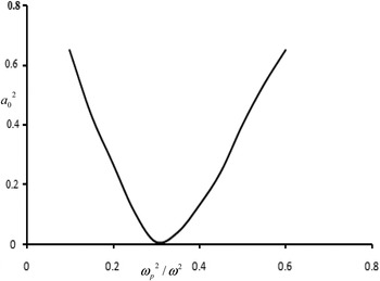
and ν0 = νg/10. It is observed that the normalized whistler amplitude decreases with ωc/ω. In Fig. 2, the variation of the normalized whistler amplitude
 $a_0^2 $
with
 $ {\rm \omega} _{\rm p}^{\rm 2} / {\rm \omega} ^{\rm 2}$
has been shown for ωc/ω = 1.31 and ν0 = νg/10. The variation possesses a nearly parabolic pattern.
Variation of normalized whistler amplitude
 $a_0^2 $
with ωc/ω for
 $ {\rm \omega} _{\rm p}^{\rm 2} / {\rm \omega} = 0.2$
and ν0 = νg/10.

Variation of normalized whistler amplitude
 $a_0^2 $
with
 $ {\rm \omega} _{\rm p}^{\rm 2} / {\rm \omega} ^{\rm 2}$
for ωc/ω = 1.3 and ν0 = νg/10.

3. DISCUSSION
The ponderomotive force associated with a one-dimensional (1D) whistler pulse is axial. For ω>ωc/2, the ponderomotive force is directed away from the intensity maximum, while for ω<ωc/2, the ponderomotive force reverses the direction and tends to pull electron toward the intensity peak. For acceleration of electrons, one requires a whistler pulse of ω>ωc/2. Maximum ponderomotive force is obtained near resonance ω = ωc/2. A pulse of ω close to ωc exerts much stronger axial ponderomotive force. In 1D, the electron gains energy during the rising front of the pulse, the rear acts as a backward ponderomotive force and slows down the electron to its original energy. Hence, to achieve energy gain the value of peak pulse amplitude should be above the threshold value. The threshold value of the whistler amplitude depends on the quantum plasma density as well as on ωc. The threshold corresponds to ν
z
= νg at the pulse peak, that is, the electron velocity is equal to the group velocity of the whistler pulse as the electron reaches the pulse peak. The threshold value of amplitude
 $(a_0^2 )$
for ωc/ω=1.31 and
 $ {\rm \omega} _{\rm p}^{\rm 2} / {\rm \omega} ^{\rm 2} = 0.3$
is 0.82. This threshold value is much greater than that obtained for classical plasma, and hence a higher intensity laser pulse is required for quantum plasma for effective acceleration. This is due to the diffraction effects induced by the quantum diffraction terms. The threshold amplitude decreases with the ratio of plasma frequency to electron cyclotron frequency, ωp/ωc. However, above the threshold amplitude, the acceleration energy decreases with ωp/ωc. The electrons gain velocities about twice the group velocity of the whistler. The threshold amplitude approches zero as ωc/ω → 1. However, the group velocity of the whistler pulse vanishes at the cyclotron resonsnce and there is no net energy gain.
ACKNOWLEDGEMENTS
This work was performed under the financial assistance from the University Grants Commission (U.G.C) India, under project no. 39-458/2010 (SR).