1 Introduction and statement of the problem

Transient flows generated by isolated/distributed sources are a topic frequently encountered in many branches of physics, such as electromagnetism (Jackson Reference Jackson2007), heat transfer (Carslaw & Jaeger Reference Carslaw and Jaeger2000) and diffusion (Crank Reference Crank2004). In the context of the fluid mechanics in porous formations (aquifers and petroleum reservoirs), transient source flows lend themselves as a very powerful diagnostic tool to determine the hydraulic properties of the formations (a classical overview can be found in Kruseman & de Ridder Reference Kruseman and de Ridder1979). Briefly, from a well (or a battery of wells) water is pumped/injected over a certain interval. The effect of such a stimulation upon the pressure distribution in the flow domain is recorded, and the hydraulic properties are identified by matching the measured pressure values against the theoretical ones.

Numerous analytical studies have contributed to solving unsteady flows in geological formations (a comprehensive collection of the classical solutions can be found in Bruggeman Reference Bruggeman1999). Common to all these analytical studies is modelling the formation as homogeneous (or at most as a sequence of homogeneous layers). However, geological formations are de facto heterogeneous with the hydraulic conductivity $K$ , in particular, varying in space quite largely (see, e.g. the data survey in Rubin Reference Rubin2003). These irregular changes have a tremendous impact upon flow (and transport) taking place in porous formations (Dagan Reference Dagan1984, Reference Dagan1987). The common (and widely accepted) approach to tackle these erratic spatial variations is a stochastic framework that regards the conductivity $K$ as a random space function (rsf) (Dagan Reference Dagan1989; Gelhar Reference Gelhar1993; Rubin Reference Rubin2003), therefore rendering stochastic the flow equation.

In the present study, we consider an unsteady flow taking place into an unbounded $d$ -dimensional domain $\unicode[STIX]{x1D6FA}_{d}$ . The flow field is generated by a given (i.e. deterministic) source function $\unicode[STIX]{x1D711}\equiv \unicode[STIX]{x1D711}(\boldsymbol{x},t)$ of finite support, and the aim here is the computation of the hydraulic head $H$ . The governing equations are the constitutive (Darcy) law

(1.1) $$\begin{eqnarray}\boldsymbol{q}(\boldsymbol{x},t)=-K(\boldsymbol{x})\unicode[STIX]{x1D735}H(\boldsymbol{x},t),\end{eqnarray}$$

relating the flux $\boldsymbol{q}$ (volumetric rate per unit cross area) to the gradient of $H$ via the conductivity $K$ , and the mass conservation equation

(1.2) $$\begin{eqnarray}S\frac{\unicode[STIX]{x2202}}{\unicode[STIX]{x2202}t}H(\boldsymbol{x},t)+\unicode[STIX]{x1D735}\boldsymbol{\cdot }\boldsymbol{q}(\boldsymbol{x},t)=\unicode[STIX]{x1D711}(\boldsymbol{x},t),\end{eqnarray}$$

where $S$ is the specific storativity that, due to its less spatial variability as compared with that of $K$ (Rubin Reference Rubin2003; Rabinovich et al. Reference Rabinovich, Barrash, Cardiff, Hochstetler, Bakhos, Dagan and Kitanidis2015; Cheng, Rabinovich & Dagan Reference Cheng, Rabinovich and Dagan2019), is regarded herein as a constant. The combination of (1.1) and (1.2) leads to the governing, parabolic-type, flow equation:

(1.3) $$\begin{eqnarray}S\frac{\unicode[STIX]{x2202}}{\unicode[STIX]{x2202}t}H(\boldsymbol{x},t)-\unicode[STIX]{x1D735}\boldsymbol{\cdot }[K(\boldsymbol{x})\unicode[STIX]{x1D735}H(\boldsymbol{x},t)]=\unicode[STIX]{x1D711}(\boldsymbol{x},t),\quad \boldsymbol{x}\in \unicode[STIX]{x1D6FA}_{d},\quad t\geqslant 0.\end{eqnarray}$$

In a homogeneous medium the problem at stake is characterized by stream lines originating from the source. The ‘distortion effect’ due to the heterogeneity of $K$ causes the stream lines to fluctuate around the ones pertaining to a homogeneous medium (i.e. a medium with $K\equiv \text{const.}$ ), similarly to a vortex-type flow where the fluctuations are determined by the uncertainty of the hydrodynamical coefficients (Landau & Lifshitz Reference Landau and Lifshitz1959). As a consequence, the hydraulic head $H$ becomes a random field, and one is interested in the computation of its ensemble moments.

Most previous studies were limited to the so-called ‘mean uniform flow’: a steady-state flow in the absence of source, which can be formally obtained from (1.3) by setting $S=\unicode[STIX]{x1D711}=0$ and by assigning a constant head gradient $-\unicode[STIX]{x1D735}H$ on the boundary $\unicode[STIX]{x2202}\unicode[STIX]{x1D6FA}_{d}$ of the flow domain (Dagan Reference Dagan1987). Although the problem of calculating the ensemble moments of $H$ satisfying (1.3) is of wide practical/theoretical concern (see, e.g. Streltsova Reference Streltsova1987; Choy Reference Choy2015), it has been studied to a lesser extent as compared with the case of the mean uniform flow (partly because of the mathematical difficulties). In fact, with the exception of Shvidler (Reference Shvidler1966), who considered the flow behaviour near and far from the source, a general approach has been formulated only recently by Neuman et al. (Reference Neuman, Tartakovsky, Wallstrom and Winter1996), Indelman (Reference Indelman1996, Reference Indelman2000) and Tartakovsky & Neuman (Reference Tartakovsky and Neuman1998b ). The main result of these studies is an effective (constitutive) law relating the mean velocity to the mean hydraulic gradient. However, knowledge of the mean values of the flow variables is not enough to characterize flow and transport in randomly heterogeneous porous media. Indeed, in order to quantify the uncertainty in the head measurements as affected by the limited knowledge of the conductivity field $K$ , the covariance $C_{H}$ is also required. Recently, this point has become particularly relevant because of new monitoring devices of pressure (see, e.g. Cardiff, Barrash & Kitanidis Reference Cardiff, Barrash and Kitanidis2013) which de facto enable one to detect the head variance $\unicode[STIX]{x1D70E}_{H}^{2}$ . As a consequence, knowledge of the latter becomes of paramount importance for identifying an aquifer’s hydraulic properties.

In order to compute $C_{H}$ , we introduce the dimensionless position $\boldsymbol{x}/\ell$ and time $t\langle K\rangle /(S\ell ^{2})$ , where $\ell$ is a characteristic length scale (that will be defined later on). In addition, we model the fluctuation $\unicode[STIX]{x1D700}(\boldsymbol{x})=1-K(\boldsymbol{x})/\langle K\rangle$ as a second-order stationary rsf with variance $\unicode[STIX]{x1D70E}^{2}$ and autocorrelation $\unicode[STIX]{x1D70C}\equiv \unicode[STIX]{x1D70C}(\boldsymbol{x})$ . Hence, substitution into (1.3) (for simplicity we retain the same notation) leads to the stochastic equation

(1.4) $$\begin{eqnarray}\frac{\unicode[STIX]{x2202}}{\unicode[STIX]{x2202}t}H(\boldsymbol{x},t)-\unicode[STIX]{x1D6FB}^{2}H(\boldsymbol{x},t)+\unicode[STIX]{x1D735}\boldsymbol{\cdot }[\unicode[STIX]{x1D700}(\boldsymbol{x})\unicode[STIX]{x1D735}H(\boldsymbol{x},t)]=\unicode[STIX]{x1D719}(\boldsymbol{x},t)\end{eqnarray}$$

(with $\unicode[STIX]{x1D711}\ell /\langle K\rangle \equiv \unicode[STIX]{x1D719}$ ). The solution of (1.4) is sought for deterministic initial and boundary conditions, i.e.

(1.5a,b ) $$\begin{eqnarray}H(\boldsymbol{x},0)\equiv H_{0}(\boldsymbol{x}),\quad \lim _{|\boldsymbol{x}|\rightarrow \infty }H(\boldsymbol{x},t)=0.\end{eqnarray}$$

Before going on, it is worth observing that in stochastic subsurface hydrology it is customary to model the log-conductivity $Y=\ln K$ as a rsf. However, the two formulations are equivalent, since one has

(1.6a-c ) $$\begin{eqnarray}\langle K\rangle =\exp \left(\langle Y\rangle +\frac{\unicode[STIX]{x1D70E}_{Y}^{2}}{2}\right),\quad \unicode[STIX]{x1D70E}^{2}=\exp (\unicode[STIX]{x1D70E}_{Y}^{2})-1,\quad \unicode[STIX]{x1D70C}(\boldsymbol{x})=\frac{\exp [\unicode[STIX]{x1D70E}_{Y}^{2}\unicode[STIX]{x1D70C}_{Y}(\boldsymbol{x})]-1}{\exp (\unicode[STIX]{x1D70E}_{Y}^{2})-1},\end{eqnarray}$$

where $\unicode[STIX]{x1D70E}_{Y}^{2}$ and $\unicode[STIX]{x1D70C}_{Y}$ are the variance and the autocorrelation of $Y$ , respectively. In addition, for the majority of real aquifers one has $\unicode[STIX]{x1D70E}_{Y}^{2}\ll 1$ (see, e.g. tables $2.1$ and $2.2$ in Rubin Reference Rubin2003), and concurrently from (1.6) it yields $\unicode[STIX]{x1D70E}^{2}\simeq \unicode[STIX]{x1D70E}_{Y}^{2}$ and $\unicode[STIX]{x1D70C}\simeq \unicode[STIX]{x1D70C}_{Y}$ . Moreover, it has been recently demonstrated (Severino Reference Severino2019) that the above (first-order) approximation can be relaxed to $\unicode[STIX]{x1D70E}_{Y}^{2}\simeq 1$ . Thus, the first-order approximation is a powerful tool for solving numerous problems of practical concern.

We also note that modelling $K$ (or alternatively $\unicode[STIX]{x1D700}$ ) as a rsf is equivalent to the approach adopted for a large variety of turbulent flows, such as flow in pipelines, density-driven flows, flow through pumps/turbines and reactive flows (a wide review can be found in Pope Reference Pope2010). The difference is that in turbulent flows the stochastic nature of the depending scalar field(s) is due to the velocity which is regarded as a given random field, whereas in the present study the random nature of the hydraulic head stems from the spatial variability of the conductivity.

A quite common approach to solve the problem at stake relies upon the method of moment equations (see, e.g. Tartakovsky & Neuman Reference Tartakovsky and Neuman1998a ,Reference Tartakovsky and Neuman b , and references therein). Although such a method is in principle simple to implement (see, e.g. Zhang Reference Zhang2002), it generally requires a very huge computational resource (Ye et al. Reference Ye, Neuman, Guadagnini and Tartakovsky2004). In contrast, analytical methods lead to direct expression of the fluctuation of the flow variables, and concurrently to the various (cross)-covariances (by ensemble averaging). Furthermore, analytical methods (although mathematically more difficult) enable one to obtain closed-form solutions which provide explicit relationships between the input parameters and the model output, therefore giving physical insight to the specific problem. Analytical results represent also a benchmark to validate the method of moment equations. In the present study, we follow this second avenue.

The paper is organized as follows. We start by formulating the mathematical problem in the context of a stochastic framework, and derive a very general (i.e. valid for any $\unicode[STIX]{x1D70C}$ and $\unicode[STIX]{x1D719}$ ) expression of the head covariance $C_{H}$ . The behaviour of $C_{H}$ is investigated in detail after adopting a specific shape for the autocorrelation function  $\unicode[STIX]{x1D70C}$ . In view of applications, we focus on the head covariance pertaining to a flow generated by a source of instantaneous and constant strength, and in particular we discuss how the spatial variability of the hydraulic conductivity influences the uncertainty of the hydraulic head. Then, we show that, in the case of flow generated by a source of constant strength, our approach leads in the large time limit to the correct steady-state version of the problem at stake. We summarize the main results of the present study in the concluding remarks.

2 General representation of the head covariance

The stochastic equation (1.4) is solved by applying Laplace transform (LT) in time and $d$ -dimensional Fourier transform (FT) in space (the latter being denoted by a tilde), i.e.

(2.1) $$\begin{eqnarray}\widehat{f}(\boldsymbol{k},s)=\int _{0}^{\infty }\int _{\unicode[STIX]{x1D6FA}_{d}}\frac{\text{d}t\,\text{d}\boldsymbol{x}}{(2\unicode[STIX]{x03C0})^{d/2}}f(\boldsymbol{x},t)\exp (-st+\jmath \boldsymbol{k}\boldsymbol{\cdot }\boldsymbol{x}).\end{eqnarray}$$

Thus, the FLT of the head satisfies the integral equation resulting from (1.4) as follows:

(2.2) $$\begin{eqnarray}\displaystyle \widehat{H}(\boldsymbol{k},s) & = & \displaystyle \left[\widehat{\unicode[STIX]{x1D719}}(\boldsymbol{k},s)+\widetilde{H}_{0}(\boldsymbol{k})+\int \frac{\text{d}\boldsymbol{p}}{(2\unicode[STIX]{x03C0})^{d/2}}\widetilde{\unicode[STIX]{x1D700}}(\boldsymbol{k}-\boldsymbol{p})\boldsymbol{k}\boldsymbol{\cdot }\boldsymbol{p}\widehat{H}(\boldsymbol{p},s)\right](k^{2}+s)^{-1}\nonumber\\ \displaystyle & = & \displaystyle (2\unicode[STIX]{x03C0})^{d/2}\widehat{G}_{(d)}(k,s)\left[\widehat{\unicode[STIX]{x1D719}}(\boldsymbol{k},s)+\widetilde{H}_{0}(\boldsymbol{k})+\int \frac{\text{d}\boldsymbol{p}}{(2\unicode[STIX]{x03C0})^{d/2}}\widetilde{\unicode[STIX]{x1D700}}(\boldsymbol{k}-\boldsymbol{p})\boldsymbol{k}\boldsymbol{\cdot }\boldsymbol{p}\widehat{H}(\boldsymbol{p},s)\right],\qquad\end{eqnarray}$$

where we have accounted for the FLT of the $d$ -dimensional Green function $G_{(d)}(x,t)$ , i.e.

(2.3) $$\begin{eqnarray}\mathtt{FLT}^{-1}\left[\frac{1}{k^{2}+s}\right]=(2t)^{-d/2}\exp \left(-\frac{x^{2}}{4t}\right)=(2\unicode[STIX]{x03C0})^{d/2}G_{(d)}(x,t).\end{eqnarray}$$

To obtain a simple expression for the covariance of $H$ , we employ (like Indelman Reference Indelman1996; Tartakovsky, Guadagnini & Riva Reference Tartakovsky, Guadagnini and Riva2003; Severino & De Bartolo Reference Severino and De Bartolo2015) a perturbation approach which provides an accurate solution for small $\unicode[STIX]{x1D70E}^{2}$ , i.e. the heterogeneous flow slightly differs from the homogeneous (mean) one, in close analogy to the ‘frozen turbulence’ approximation (e.g. Wilczek, Stevens & Meneveau Reference Wilczek, Stevens and Meneveau2015; Saw et al. Reference Saw, Debue, Kuzzay, Daviaud and Dubrulle2018). Thus, the solution of (2.2) is sought by expanding $\widehat{H}$ in the following asymptotic series:

(2.4) $$\begin{eqnarray}\widehat{H}(\boldsymbol{k},s)=\widehat{H}^{(0)}(\boldsymbol{k},s)+\widehat{H}^{(1)}(\boldsymbol{k},s)+\cdots ,\quad \widehat{H}^{(n)}=O(\widetilde{\unicode[STIX]{x1D700}}^{n}).\end{eqnarray}$$

Then, substitution of (2.4) into (2.2) and collecting terms of the same order lead to the FLT of the head fluctuation (first-order approximation):

(2.5) $$\begin{eqnarray}\widehat{H}^{(1)}(\boldsymbol{k},s)=k_{m}\widehat{G}_{(d)}(k,s)\int \text{d}\boldsymbol{p}\widetilde{\unicode[STIX]{x1D700}}(\boldsymbol{k}-\boldsymbol{p})p_{m}\widehat{H}^{(0)}(\boldsymbol{p},s),\end{eqnarray}$$

where $\widehat{H}^{(0)}(\boldsymbol{k},s)=(2\unicode[STIX]{x03C0})^{d/2}\widehat{G}_{(d)}(k,s)[\widehat{\unicode[STIX]{x1D719}}(\boldsymbol{k},s)+\widetilde{H}_{0}(\boldsymbol{k})]$ .

Prior to the explicit derivation of $C_{H}$ , we wish to discuss a relevant property of the head fluctuation. To this end, we compute this latter by inverting first its LT, i.e.

(2.6) $$\begin{eqnarray}\widetilde{H}^{(1)}(\boldsymbol{k},t)=k_{m}\int _{0}^{t}\text{d}\unicode[STIX]{x1D70F}\widetilde{G}_{(d)}(k,t-\unicode[STIX]{x1D70F})\int \text{d}\boldsymbol{p}\widetilde{\unicode[STIX]{x1D700}}(\boldsymbol{k}-\boldsymbol{p})p_{m}\widetilde{H}^{(0)}(\boldsymbol{p},\unicode[STIX]{x1D70F}),\end{eqnarray}$$

and subsequently the resulting FT (2.6), to come up with

(2.7) $$\begin{eqnarray}H^{(1)}(\boldsymbol{x},t)=-\int _{0}^{t}\text{d}\unicode[STIX]{x1D70F}\int _{\unicode[STIX]{x1D6FA}_{d}}\text{d}\bar{\boldsymbol{x}}\unicode[STIX]{x1D700}(\bar{\boldsymbol{x}})\frac{\unicode[STIX]{x2202}}{\unicode[STIX]{x2202}\bar{x}_{m}}H^{(0)}(\bar{\boldsymbol{x}},\unicode[STIX]{x1D70F})\frac{\unicode[STIX]{x2202}}{\unicode[STIX]{x2202}\unicode[STIX]{x1D709}_{m}}G_{(d)}(\unicode[STIX]{x1D709},t-\unicode[STIX]{x1D70F})\end{eqnarray}$$

$(\unicode[STIX]{x1D743}\equiv \boldsymbol{x}-\bar{\boldsymbol{x}})$ . Accounting for the chain rule of derivation $\unicode[STIX]{x2202}/\unicode[STIX]{x2202}x_{m}\equiv (x_{m}/x)(\unicode[STIX]{x2202}/\unicode[STIX]{x2202}x)$ yields

(2.8) $$\begin{eqnarray}H^{(1)}(\boldsymbol{x},t)=\frac{1}{2}\int _{0}^{t}\frac{\text{d}\unicode[STIX]{x1D70F}}{t-\unicode[STIX]{x1D70F}}\int _{\unicode[STIX]{x1D6FA}_{d}}\frac{\text{d}\bar{\boldsymbol{x}}}{\bar{x}}\unicode[STIX]{x1D700}(\bar{\boldsymbol{x}})\frac{\unicode[STIX]{x2202}}{\unicode[STIX]{x2202}\bar{x}}H^{(0)}(\bar{\boldsymbol{x}},\unicode[STIX]{x1D70F})\bar{\boldsymbol{x}}\boldsymbol{\cdot }(\boldsymbol{x}-\bar{\boldsymbol{x}})G_{(d)}(|\boldsymbol{x}-\bar{\boldsymbol{x}}|,t-\unicode[STIX]{x1D70F}).\end{eqnarray}$$

Similarly, the leading-order term is obtained by inverting $\widehat{H}^{(0)}$ , the final result being

(2.9) $$\begin{eqnarray}H^{(0)}(\boldsymbol{x},t)=\int _{0}^{t}\int _{\unicode[STIX]{x1D6FA}_{d}}\text{d}\unicode[STIX]{x1D70F}\,\text{d}\bar{\boldsymbol{x}}\unicode[STIX]{x1D719}(\bar{\boldsymbol{x}},\unicode[STIX]{x1D70F})G_{(d)}(|\boldsymbol{x}-\bar{\boldsymbol{x}}|,t-\unicode[STIX]{x1D70F})+\int _{\unicode[STIX]{x1D6FA}_{d}}\text{d}\bar{\boldsymbol{x}}H_{0}(\bar{\boldsymbol{x}})G_{(d)}(|\boldsymbol{x}-\bar{\boldsymbol{x}}|,t).\end{eqnarray}$$

The fundamental implication of (2.8) is that

(2.10) $$\begin{eqnarray}\int _{\unicode[STIX]{x1D6FA}_{d}}\text{d}\boldsymbol{x}H^{(1)}(\boldsymbol{x},t)=\frac{1}{2}\int _{0}^{t}\frac{\text{d}\unicode[STIX]{x1D70F}}{\unicode[STIX]{x1D70F}}\int _{\unicode[STIX]{x1D6FA}_{d}}\text{d}\bar{\boldsymbol{x}}\unicode[STIX]{x1D700}(\bar{\boldsymbol{x}})\frac{\unicode[STIX]{x2202}}{\unicode[STIX]{x2202}\bar{x}}H^{(0)}(\bar{\boldsymbol{x}},t-\unicode[STIX]{x1D70F})\frac{\bar{x}_{m}}{\bar{x}}\int _{\unicode[STIX]{x1D6FA}_{d}}\text{d}\boldsymbol{x}x_{m}G_{(d)}(x,\unicode[STIX]{x1D70F})=0,\end{eqnarray}$$

for any $d$ and $t$ (it is recalled that the Green function is an even function of the position $\boldsymbol{x}$ ). The property (2.10) is a consequence of the mass conservation law arising from (2.9), i.e.

(2.11) $$\begin{eqnarray}\int _{\unicode[STIX]{x1D6FA}_{d}}\text{d}\boldsymbol{x}H^{(0)}(\boldsymbol{x},t)=\int _{\unicode[STIX]{x1D6FA}_{d}}\int _{0}^{t}\text{d}\boldsymbol{x}\,\text{d}\unicode[STIX]{x1D70F}\unicode[STIX]{x1D719}(\boldsymbol{x},\unicode[STIX]{x1D70F})+\int _{\unicode[STIX]{x1D6FA}_{d}}\text{d}\boldsymbol{x}H_{0}(\boldsymbol{x})\equiv \text{const.},\end{eqnarray}$$

together with the fact that $\int _{\unicode[STIX]{x1D6FA}_{d}}\text{d}\boldsymbol{x}G_{(d)}(x,t)=1$ , and $H_{0}\in {\mathcal{L}}^{1}(\unicode[STIX]{x1D6FA}_{d})$ . In a different manner one can claim that $\unicode[STIX]{x1D6FA}_{d}$ can be sought as a collection of subdomains in which the fluctuation $H^{(1)}$ adjusts to satisfy (2.10). In addition, from (2.11) it is seen that the property (2.10) stems only from the deterministic nature of the initial/boundary conditions (1.5), and therefore it is valid for a broad class of configurations. The property (2.10) can be used as benchmark to check, for instance, the consistency of numerical schemes accounting for the presence of more complex boundary conditions.

We can now compute the head covariance $C_{H}(\boldsymbol{x},\boldsymbol{y},t)\equiv \langle H^{(1)}(\boldsymbol{x},t)H^{(1)}(\boldsymbol{y},t)\rangle$ . Thus, starting from (2.8) one has

(2.12) $$\begin{eqnarray}\displaystyle & & \displaystyle C_{H}(\boldsymbol{x},\boldsymbol{y},t)=\frac{\unicode[STIX]{x1D70E}^{2}}{4}\int _{0}^{t}\int _{0}^{t}\frac{\text{d}\unicode[STIX]{x1D70F}^{\prime }\text{d}\unicode[STIX]{x1D70F}^{\prime \prime }}{(t-\unicode[STIX]{x1D70F}^{\prime })(t-\unicode[STIX]{x1D70F}^{\prime \prime })}\int _{\unicode[STIX]{x1D6FA}_{d}}\text{d}\bar{\boldsymbol{x}}\unicode[STIX]{x1D70C}(\bar{\boldsymbol{x}})\int _{\unicode[STIX]{x1D6FA}_{d}}\text{d}\bar{\boldsymbol{y}}{\dot{H}}^{(0)}(\bar{\boldsymbol{x}}+\bar{\boldsymbol{y}},\unicode[STIX]{x1D70F}^{\prime }){\dot{H}}^{(0)}(\bar{\boldsymbol{y}},\unicode[STIX]{x1D70F}^{\prime \prime })\nonumber\\ \displaystyle & & \displaystyle \quad \times \,(\bar{\boldsymbol{x}}+\bar{\boldsymbol{y}})\boldsymbol{\cdot }(\bar{\boldsymbol{x}}+\bar{\boldsymbol{y}}-\boldsymbol{x})\bar{\boldsymbol{y}}\boldsymbol{\cdot }(\bar{\boldsymbol{y}}-\boldsymbol{y})G_{(d)}(|\bar{\boldsymbol{x}}+\bar{\boldsymbol{y}}-\boldsymbol{x}|,t-\unicode[STIX]{x1D70F}^{\prime })G_{(d)}(|\bar{\boldsymbol{y}}-\boldsymbol{y}|,t-\unicode[STIX]{x1D70F}^{\prime \prime }),\nonumber\\ \displaystyle & & \displaystyle\end{eqnarray}$$

where we have set ${\dot{f}}(\boldsymbol{x},t)\equiv (1/x)(\unicode[STIX]{x2202}/\unicode[STIX]{x2202}x)f(\boldsymbol{x},t)$ . Overall, the covariance (2.12) is expressed via $2(d+1)$ quadratures, a task which is computer-demanding (see, e.g. Riva et al. Reference Riva, Guadagnini, Neuman and Franzetti2001) and it may be prone to numerical inaccuracies. Nevertheless, if the functional shape of $\unicode[STIX]{x1D70C}$ and $H^{(0)}$ is such that one can analytically compute the spatial integrals on the right-hand side of (2.12), then the evaluation of $C_{H}$ becomes computationally affordable and accurate.

To summarize results achieved so far, a closed (analytical) form, first-order approximation of the head fluctuation $H^{(1)}\equiv H^{(1)}(\boldsymbol{x},t)$ in transient source flows through weakly heterogeneous porous media has been derived for the first time. Unlike the method of moment equations, such an expression leads straightforwardly (i.e. without resorting to any multidimensional partial differential equation) to an analytical expression of the head covariance requiring only simple quadratures to be computed. We have then proved (2.10) stating that $\unicode[STIX]{x1D6FA}_{d}$ can be decomposed into subdomains where $H^{(1)}$ is positive/negative in order to satisfy mass conservation. This property is relevant for checking more involved numerical schemes. Finally, we have derived a very general, i.e. valid for any $H^{(0)}$ and autocorrelation $\unicode[STIX]{x1D70C}$ , expression of the head covariance (2.12).

The remainder of the paper is devoted to the explicit evaluation of $C_{H}$ for some cases which are relevant for applications (typically pumping tests) at both regional (i.e. two-dimensional) scale and formation (i.e. three-dimensional) scale.

3 Flow at regional scale $(d=2)$

We are concerned with modelling of flow at regional scale. In this case the conductivity is sought as upscaled over the aquifer’s thickness and a large horizontal area (see Dagan Reference Dagan1989, for details). As a consequence, flow becomes two-dimensional. The majority of previous works were limited to groundwater-type conditions (see, e.g. Dagan & Rubin Reference Dagan and Rubin1988; Rubin & Dagan Reference Rubin and Dagan1988, Reference Rubin and Dagan1989), whereas it is only later that analysis has been extended to flow (e.g. Dagan & Lessoff Reference Dagan and Lessoff2007; Severino Reference Severino2011b ) and transport (e.g. Severino, Santini & Sommella Reference Severino, Santini and Sommella2011) processes taking place in radial-type configurations.

3.1 Source of instantaneous strength

The importance of flows generated by a source of instantaneous strength stems from the fact that the specific storativity $S[\text{m}^{-1}]\sim O(10^{-6}/10^{-2})$ multiplies the derivative of the head with respect to the time $t$ . As a consequence, the impact of $S$ upon the head distribution is significant only at the very beginning when the variations of the head with time are very high, and concurrently $S\unicode[STIX]{x2202}H/\unicode[STIX]{x2202}t\sim O(1)$ . For this reason, in order to acquire measurements which are successful to identify the specific storativity, it has been suggested by Cardiff, Barrash & Kitanidis (Reference Cardiff, Barrash and Kitanidis2012) and Cardiff et al. (Reference Cardiff, Barrash and Kitanidis2013) to use during a pumping test a discharge which is rapidly changing with time. It is therefore interesting to analyse the uncertainty quantification of a flow generated by a source whose strength behaves (in time) like a Dirac pulse.

In this case the homogeneous head $H^{(0)}$ is obtained by computing the quadratures (2.9) with $\unicode[STIX]{x1D719}(\boldsymbol{x},t)\equiv \unicode[STIX]{x1D6FF}(\boldsymbol{x})\unicode[STIX]{x1D6FF}(t)$ and zero initial/boundary conditions, thus leading to $H^{(0)}\equiv G_{(2)}$ . The resulting covariance (2.12) is conveniently rewritten as

(3.1) $$\begin{eqnarray}C_{H}(\boldsymbol{x},\boldsymbol{y},t)=\left(\frac{\unicode[STIX]{x1D70E}}{4\unicode[STIX]{x03C0}}\right)^{2}\int _{0}^{t}\int _{0}^{t}\text{d}\unicode[STIX]{x1D70F}^{\prime }\text{d}\unicode[STIX]{x1D70F}^{\prime \prime }\frac{G_{(2)}(x,t-\unicode[STIX]{x1D70F}^{\prime })}{(t-\unicode[STIX]{x1D70F}^{\prime })\unicode[STIX]{x1D70F}^{\prime 2}}\frac{G_{(2)}(y,t-\unicode[STIX]{x1D70F}^{\prime \prime })}{(t-\unicode[STIX]{x1D70F}^{\prime \prime })\unicode[STIX]{x1D70F}^{\prime \prime 2}}\unicode[STIX]{x1D6F6}_{\unicode[STIX]{x1D6FF}}(a,\unicode[STIX]{x1D6FC};b\boldsymbol{x},\unicode[STIX]{x1D6FD}\boldsymbol{y}),\end{eqnarray}$$

(3.2) $$\begin{eqnarray}\displaystyle \unicode[STIX]{x1D6F6}_{\unicode[STIX]{x1D6FF}}(a,\unicode[STIX]{x1D6FC};b\boldsymbol{x},\unicode[STIX]{x1D6FD}\boldsymbol{y}) & = & \displaystyle \left(\frac{\unicode[STIX]{x2202}}{\unicode[STIX]{x2202}a}+\frac{\unicode[STIX]{x2202}}{\unicode[STIX]{x2202}b}\right)\left(\frac{\unicode[STIX]{x2202}}{\unicode[STIX]{x2202}\unicode[STIX]{x1D6FC}}+\frac{\unicode[STIX]{x2202}}{\unicode[STIX]{x2202}\unicode[STIX]{x1D6FD}}\right)\int _{\unicode[STIX]{x1D6FA}_{2}}\int _{\unicode[STIX]{x1D6FA}_{2}}\text{d}\bar{\boldsymbol{x}}\,\text{d}\bar{\boldsymbol{y}}\unicode[STIX]{x1D70C}(\bar{\boldsymbol{x}}-\bar{\boldsymbol{y}})\nonumber\\ \displaystyle & & \displaystyle \times \,\exp (-a\bar{x}^{2}+b\boldsymbol{x}\boldsymbol{\cdot }\bar{\boldsymbol{x}}-\unicode[STIX]{x1D6FC}\bar{y}^{2}+\unicode[STIX]{x1D6FD}\boldsymbol{y}\boldsymbol{\cdot }\bar{\boldsymbol{y}}),\end{eqnarray}$$

where $a\equiv t/(4(t-\unicode[STIX]{x1D70F}^{\prime })\unicode[STIX]{x1D70F}^{\prime })$ and $b\equiv 1/(2(t-\unicode[STIX]{x1D70F}^{\prime }))$ , whereas $\unicode[STIX]{x1D6FC}$ and $\unicode[STIX]{x1D6FD}$ are obtained by replacing $\unicode[STIX]{x1D70F}^{\prime }\rightarrow \unicode[STIX]{x1D70F}^{\prime \prime }$ into $a$ and $b$ , respectively. The tremendous advantage (from the computational point of view) related to the representation (3.1)–(3.2) is that the ‘dot products’ have been absorbed into the sequence of derivatives with respect to the fictitious variables $a$ , $b$ , $\unicode[STIX]{x1D6FC}$ and $\unicode[STIX]{x1D6FD}$ . A similar approach was employed by Indelman (Reference Indelman2000) to compute the mean Green function in the same configuration.

Overall, the covariance (3.1) is expressed via six quadratures, a computationally demanding task which is generally prone to numerical inaccuracies. Nevertheless, if the functional shape of $\unicode[STIX]{x1D70C}$ is such that one can compute analytically the $\unicode[STIX]{x1D6F6}_{\unicode[STIX]{x1D6FF}}$ function, then the evaluation of $C_{H}$ is reduced to two quadratures solely, therefore becoming computationally affordable and accurate. Towards this aim, we consider hereafter a Gaussian $\unicode[STIX]{x1D70C}(\boldsymbol{x})=\exp [-(|\boldsymbol{x}|/\ell )^{2}]$ , where $\ell$ is the correlation length (hereafter adopted as characteristic scale), which is related to correlation length $I_{Y}$ of $Y\equiv \ln K$ by the relationship $I_{Y}=\ell \sqrt{\unicode[STIX]{x03C0}}/2$ (Dagan Reference Dagan1989). Such a choice for $\unicode[STIX]{x1D70C}$ is supported by the experimental findings (see, e.g. tables $2.1$ and $2.2$ in Rubin Reference Rubin2003). Thus, for Gaussian $\unicode[STIX]{x1D70C}$ the spatial quadratures appearing in (3.2) are analytically evaluated, i.e.

(3.3) $$\begin{eqnarray}\displaystyle & & \displaystyle \int _{\unicode[STIX]{x1D6FA}_{2}}\int _{\unicode[STIX]{x1D6FA}_{2}}\text{d}\bar{\boldsymbol{x}}\,\text{d}\bar{\boldsymbol{y}}\unicode[STIX]{x1D70C}(\bar{\boldsymbol{x}}-\bar{\boldsymbol{y}})\exp (-a\bar{x}^{2}+b\boldsymbol{x}\boldsymbol{\cdot }\bar{\boldsymbol{x}}-\unicode[STIX]{x1D6FC}\bar{y}^{2}+\unicode[STIX]{x1D6FD}\boldsymbol{y}\boldsymbol{\cdot }\bar{\boldsymbol{y}})=\frac{1}{16(\bar{a}\bar{\unicode[STIX]{x1D6FC}}-1)}\nonumber\\ \displaystyle & & \displaystyle \quad \times \,\exp \left[\frac{\bar{\unicode[STIX]{x1D6FC}}(bx)^{2}+\bar{a}(\unicode[STIX]{x1D6FD}y)^{2}+2b\unicode[STIX]{x1D6FD}\boldsymbol{x}\boldsymbol{\cdot }\boldsymbol{y}}{4(\bar{a}\bar{\unicode[STIX]{x1D6FC}}-1)}\right],\end{eqnarray}$$

where we have set

(3.4a,b ) $$\begin{eqnarray}\bar{a}=\frac{t+4(t-\unicode[STIX]{x1D70F}^{\prime })\unicode[STIX]{x1D70F}^{\prime }}{4(t-\unicode[STIX]{x1D70F}^{\prime })\unicode[STIX]{x1D70F}^{\prime }}=\frac{{\mathcal{T}}^{\prime }}{4(t-\unicode[STIX]{x1D70F}^{\prime })\unicode[STIX]{x1D70F}^{\prime }},\quad \bar{\unicode[STIX]{x1D6FC}}=\frac{t+4(t-\unicode[STIX]{x1D70F}^{\prime \prime })\unicode[STIX]{x1D70F}^{\prime \prime }}{4(t-\unicode[STIX]{x1D70F}^{\prime \prime })\unicode[STIX]{x1D70F}^{\prime \prime }}=\frac{{\mathcal{T}}^{\prime \prime }}{4(t-\unicode[STIX]{x1D70F}^{\prime \prime })\unicode[STIX]{x1D70F}^{\prime \prime }}.\end{eqnarray}$$

Hence, from (3.1)–(3.3) one finally has (after carrying out the required differentiations)

(3.5) $$\begin{eqnarray}\displaystyle & \displaystyle C_{H}(\boldsymbol{x},\boldsymbol{y},t)=\left(\frac{\unicode[STIX]{x1D70E}}{4\unicode[STIX]{x03C0}t}\right)^{2}\int _{0}^{t}\int _{0}^{t}\frac{\text{d}\unicode[STIX]{x1D70F}^{\prime }\text{d}\unicode[STIX]{x1D70F}^{\prime \prime }}{\mathtt{T}^{2}}{\mathcal{C}}_{\unicode[STIX]{x1D6FF}}(\unicode[STIX]{x1D70F}^{\prime },\unicode[STIX]{x1D70F}^{\prime \prime })\exp \left(-\frac{x^{2}t_{x}+y^{2}t_{y}-8\boldsymbol{x}\boldsymbol{\cdot }\boldsymbol{y}\unicode[STIX]{x1D70F}^{\prime }\unicode[STIX]{x1D70F}^{\prime \prime }}{4t\mathtt{T}}\right),\quad & \displaystyle\end{eqnarray}$$

(3.6) $$\begin{eqnarray}\displaystyle & \displaystyle t_{x}=(1+4\unicode[STIX]{x1D70F}^{\prime }){\mathcal{T}}^{\prime \prime }-16\unicode[STIX]{x1D70F}^{\prime }(t-\unicode[STIX]{x1D70F}^{\prime \prime })\unicode[STIX]{x1D70F}^{\prime \prime }=t(1+4\unicode[STIX]{x1D70F}^{\prime })+4(t-\unicode[STIX]{x1D70F}^{\prime \prime })\unicode[STIX]{x1D70F}^{\prime \prime }, & \displaystyle\end{eqnarray}$$

(3.7) $$\begin{eqnarray}\displaystyle & \displaystyle t_{y}=(1+4\unicode[STIX]{x1D70F}^{\prime \prime }){\mathcal{T}}^{\prime }-16\unicode[STIX]{x1D70F}^{\prime }(t-\unicode[STIX]{x1D70F}^{\prime })\unicode[STIX]{x1D70F}^{\prime \prime }=t(1+4\unicode[STIX]{x1D70F}^{\prime \prime })+4(t-\unicode[STIX]{x1D70F}^{\prime })\unicode[STIX]{x1D70F}^{\prime }, & \displaystyle\end{eqnarray}$$

where $\mathtt{T}\equiv t+4(t-\unicode[STIX]{x1D70F}^{\prime })\unicode[STIX]{x1D70F}^{\prime }+4(t-\unicode[STIX]{x1D70F}^{\prime \prime })\unicode[STIX]{x1D70F}^{\prime \prime }$ , whereas the function ${\mathcal{C}}_{\unicode[STIX]{x1D6FF}}\equiv {\mathcal{C}}_{\unicode[STIX]{x1D6FF}}(\unicode[STIX]{x1D70F}^{\prime },\unicode[STIX]{x1D70F}^{\prime \prime })$ is given by

(3.8) $$\begin{eqnarray}\displaystyle & & \displaystyle {\mathcal{C}}_{\unicode[STIX]{x1D6FF}}(\unicode[STIX]{x1D70F}^{\prime },\unicode[STIX]{x1D70F}^{\prime \prime })\nonumber\\ \displaystyle & & \displaystyle =1+{\displaystyle \frac{32}{t\mathtt{T}}}(t-\unicode[STIX]{x1D70F}^{\prime })\unicode[STIX]{x1D70F}^{\prime }(t-\unicode[STIX]{x1D70F}^{\prime \prime })\unicode[STIX]{x1D70F}^{\prime \prime }+{\displaystyle \frac{x^{2}}{4(t\mathtt{T})^{2}}}\{\!16\unicode[STIX]{x1D70F}^{\prime 2}(t-\unicode[STIX]{x1D70F}^{\prime \prime })\unicode[STIX]{x1D70F}^{\prime \prime }[\!3{\mathcal{T}}^{\prime \prime }+16(t-\unicode[STIX]{x1D70F}^{\prime })\unicode[STIX]{x1D70F}^{\prime \prime }\nonumber\\ \displaystyle & & \displaystyle \times \,(t-\unicode[STIX]{x1D70F}^{\prime \prime })\!]-(1+4\unicode[STIX]{x1D70F}^{\prime }){\mathcal{T}}^{\prime }{\mathcal{T}}^{\prime \prime 2}\!\}+{\displaystyle \frac{y^{2}}{4(t\mathtt{T})^{2}}}\{\!16(t-\unicode[STIX]{x1D70F}^{\prime })\unicode[STIX]{x1D70F}^{\prime }\unicode[STIX]{x1D70F}^{\prime \prime 2}[3{\mathcal{T}}^{\prime }+16(t-\unicode[STIX]{x1D70F}^{\prime })\unicode[STIX]{x1D70F}^{\prime }(t-\unicode[STIX]{x1D70F}^{\prime \prime })]\nonumber\\ \displaystyle & & \displaystyle -\,(1+4\unicode[STIX]{x1D70F}^{\prime \prime }){\mathcal{T}}^{\prime 2}{\mathcal{T}}^{\prime \prime }\!\}+\,\boldsymbol{x}\boldsymbol{\cdot }\boldsymbol{y}\left\{{\displaystyle \frac{1}{2}}-{\displaystyle \frac{2}{t\mathtt{T}}}(\unicode[STIX]{x1D70F}^{\prime }{\mathcal{T}}^{\prime \prime }+\unicode[STIX]{x1D70F}^{\prime \prime }{\mathcal{T}}^{\prime })+2\frac{\unicode[STIX]{x1D70F}^{\prime }\unicode[STIX]{x1D70F}^{\prime \prime }}{(t\mathtt{T})^{2}} [\!16(t-\unicode[STIX]{x1D70F}^{\prime })\unicode[STIX]{x1D70F}^{\prime }(t-\unicode[STIX]{x1D70F}^{\prime \prime })\unicode[STIX]{x1D70F}^{\prime \prime }\right.\nonumber\\ \displaystyle & & \displaystyle +\left.3{\mathcal{T}}^{\prime }{\mathcal{T}}^{\prime \prime }\!]\right\}\!+\frac{x^{4}}{(t\mathtt{T})^{3}}\unicode[STIX]{x1D70F}^{\prime 2}(t\!-\unicode[STIX]{x1D70F}^{\prime \prime })\unicode[STIX]{x1D70F}^{\prime \prime }{\mathcal{T}}^{\prime \prime }[16\unicode[STIX]{x1D70F}^{\prime }(t\!-\!\unicode[STIX]{x1D70F}^{\prime \prime })\unicode[STIX]{x1D70F}^{\prime \prime }\!-(1\!+\!4\unicode[STIX]{x1D70F}^{\prime }){\mathcal{T}}^{\prime \prime }]\!+{\displaystyle \frac{y^{4}}{(t\mathtt{T})^{3}}}(t\!-\!\unicode[STIX]{x1D70F}^{\prime })\unicode[STIX]{x1D70F}^{\prime }\unicode[STIX]{x1D70F}^{\prime \prime 2}{\mathcal{T}}^{\prime }\nonumber\\ \displaystyle & & \displaystyle \times \,[16(t-\unicode[STIX]{x1D70F}^{\prime })\unicode[STIX]{x1D70F}^{\prime }\unicode[STIX]{x1D70F}^{\prime \prime }\!-(1\!+4\unicode[STIX]{x1D70F}^{\prime \prime }){\mathcal{T}}^{\prime }]\!+{\displaystyle \frac{(\boldsymbol{x}\boldsymbol{\cdot }\boldsymbol{y})^{2}}{(t\mathtt{T})^{3}}}\unicode[STIX]{x1D70F}^{\prime }\unicode[STIX]{x1D70F}^{\prime \prime }[({\mathcal{T}}^{\prime \prime }\!-2\unicode[STIX]{x1D70F}^{\prime \prime }){\mathcal{T}}^{\prime }\!-16(t\!-\unicode[STIX]{x1D70F}^{\prime })\unicode[STIX]{x1D70F}^{\prime }(t\!-\unicode[STIX]{x1D70F}^{\prime \prime })\unicode[STIX]{x1D70F}^{\prime \prime }]\nonumber\\ \displaystyle & & \displaystyle \displaystyle \times \,[({\mathcal{T}}^{\prime }-2\unicode[STIX]{x1D70F}^{\prime }){\mathcal{T}}^{\prime \prime }-\!16(t\!-\unicode[STIX]{x1D70F}^{\prime })\unicode[STIX]{x1D70F}^{\prime }(t\!-\unicode[STIX]{x1D70F}^{\prime \prime })\unicode[STIX]{x1D70F}^{\prime \prime }]+x^{2}{\displaystyle \frac{\boldsymbol{x}\boldsymbol{\cdot }\boldsymbol{y}}{4(t\mathtt{T})^{2}}}\unicode[STIX]{x1D70F}^{\prime }\left\{\!16\unicode[STIX]{x1D70F}^{\prime }(t\!-\unicode[STIX]{x1D70F}^{\prime \prime })\unicode[STIX]{x1D70F}^{\prime \prime 2}\left(\!{\displaystyle \frac{2\unicode[STIX]{x1D70F}^{\prime }}{t\mathtt{T}}}{\mathcal{T}}^{\prime \prime }-\!1\!\right)\right.\nonumber\\ \displaystyle & & \displaystyle +\left.{\mathcal{T}}^{\prime \prime }[16\unicode[STIX]{x1D70F}^{\prime }(t-\unicode[STIX]{x1D70F}^{\prime \prime })\unicode[STIX]{x1D70F}^{\prime \prime }-(1+4\unicode[STIX]{x1D70F}^{\prime }){\mathcal{T}}^{\prime \prime }]\left(\frac{2\unicode[STIX]{x1D70F}^{\prime \prime }}{t\mathtt{T}}{\mathcal{T}}^{\prime }-1\right)\right\}+y^{2}{\displaystyle \frac{\boldsymbol{x}\boldsymbol{\cdot }\boldsymbol{y}}{4(t\mathtt{T})^{2}}}\unicode[STIX]{x1D70F}^{\prime \prime }\left\{16(t-\unicode[STIX]{x1D70F}^{\prime })\unicode[STIX]{x1D70F}^{\prime 2}\unicode[STIX]{x1D70F}^{\prime \prime }\right.\nonumber\\ \displaystyle & & \displaystyle \times \left.\left({\displaystyle \frac{2\unicode[STIX]{x1D70F}^{\prime \prime }}{t\mathtt{T}}}{\mathcal{T}}^{\prime }-1\right)+{\mathcal{T}}^{\prime }[16(t-\unicode[STIX]{x1D70F}^{\prime })\unicode[STIX]{x1D70F}^{\prime }\unicode[STIX]{x1D70F}^{\prime \prime }-(1+4\unicode[STIX]{x1D70F}^{\prime \prime }){\mathcal{T}}^{\prime }]\left(\frac{2\unicode[STIX]{x1D70F}^{\prime }}{t\mathtt{T}}{\mathcal{T}}^{\prime \prime }-1\right)\right\},\nonumber\\ \displaystyle & & \displaystyle\end{eqnarray}$$

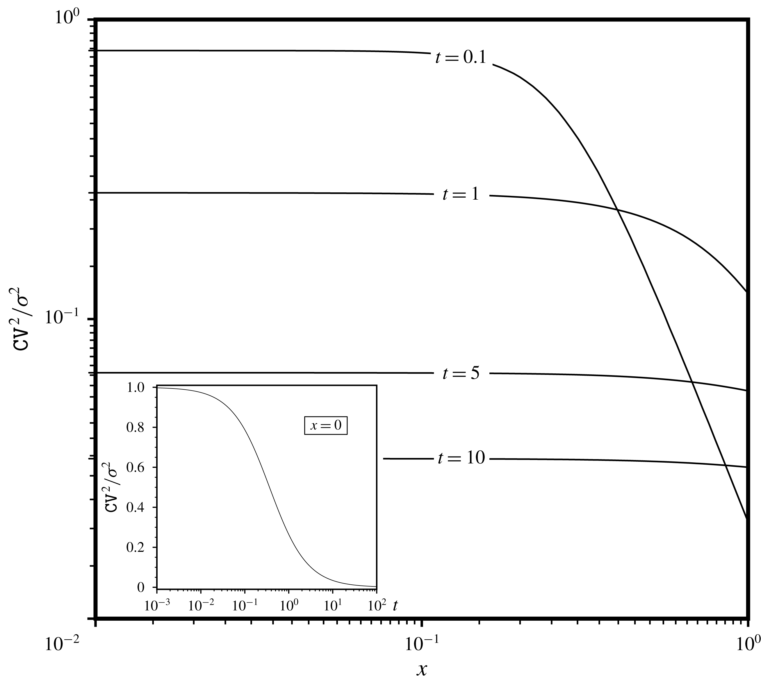
with ${\mathcal{T}}^{\prime }$ and ${\mathcal{T}}^{\prime \prime }$ defined in (3.4). To grasp the impact of the medium’s heterogeneity upon the head spatial distribution, in figure 1 we depict $\mathtt{CV}^{2}\equiv \unicode[STIX]{x1D70E}_{H}^{2}(x,t)/G_{(2)}^{2}(x,t)$ as a function of the distance $x$ from the source, and some values of the time $t$ . The constant value of $\mathtt{CV}^{2}$ for $x\ll 1$ suggests that $\unicode[STIX]{x1D70E}_{H}=O(G_{(2)})$ in the near field. In particular, at the source $x=0$ (inset in figure 1) one has $\unicode[STIX]{x1D70E}_{H}^{2}\equiv \unicode[STIX]{x1D70E}^{2}G_{(2)}^{2}$ at the very early times. Indeed, it easy to show that

(3.9) $$\begin{eqnarray}\displaystyle & \displaystyle \lim _{t\rightarrow 0}\mathtt{CV}^{2}(0,t)\equiv \unicode[STIX]{x1D70E}^{2}\lim _{t\rightarrow 0}\int _{0}^{1}\int _{0}^{1}\frac{\text{d}\unicode[STIX]{x1D70F}^{\prime }\,\text{d}\unicode[STIX]{x1D70F}^{\prime \prime }}{\bar{\mathtt{T}}^{2}}\left[1+\frac{32}{\bar{\mathtt{T}}}t^{2}(1-\unicode[STIX]{x1D70F}^{\prime })\unicode[STIX]{x1D70F}^{\prime }(1-\unicode[STIX]{x1D70F}^{\prime \prime })\unicode[STIX]{x1D70F}^{\prime \prime }\right]=\unicode[STIX]{x1D70E}^{2}, & \displaystyle\end{eqnarray}$$

(3.10) $$\begin{eqnarray}\displaystyle & \displaystyle \bar{\mathtt{T}}=1+4t[(1-\unicode[STIX]{x1D70F}^{\prime })\unicode[STIX]{x1D70F}^{\prime }+(1-\unicode[STIX]{x1D70F}^{\prime \prime })\unicode[STIX]{x1D70F}^{\prime \prime }]. & \displaystyle\end{eqnarray}$$

Instead, $\mathtt{CV}^{2}/\unicode[STIX]{x1D70E}^{2}$ decays (for fixed $x$ ) with time. In order to discuss the behaviour of the head variance close to the source, we compute the specific (per unit length) volumetric rate there, i.e.

(3.11) $$\begin{eqnarray}Q=\int _{0}^{\infty }\int _{\unicode[STIX]{x1D6FA}_{r}}\text{d}t\,\text{d}\boldsymbol{x}\unicode[STIX]{x1D719}(\boldsymbol{x},t)=\text{const.},\end{eqnarray}$$

where $\unicode[STIX]{x1D6FA}_{r}$ is an annulus of very small radius $r$ surrounding the source. As a consequence, the radial flux $q_{r}\equiv Q/(2\unicode[STIX]{x03C0}r)$ is also constant, and by virtue of constitutive law (1.1) one has (after ensemble averaging)

(3.12) $$\begin{eqnarray}\frac{q_{r}}{\langle K\rangle }\left\langle \frac{1}{1-\unicode[STIX]{x1D700}}\right\rangle ^{-1}=-\frac{\unicode[STIX]{x2202}}{\unicode[STIX]{x2202}r}\langle H\rangle .\end{eqnarray}$$

Thus, in the close vicinity of the source the mean head $\langle H\rangle$ can be computed by regarding the flow domain as a unit of (harmonic) conductivity $K_{H}\equiv \langle K\rangle \langle (1-\unicode[STIX]{x1D700})^{-1}\rangle ^{-1}$ . Such a result was derived in the past for a steady source flow of constant strength (Dagan Reference Dagan1989), and subsequently proved to be correct also for unsteady flows generated by a source of constant strength (Indelman Reference Indelman1996, Reference Indelman2003). Here it is extended to flows generated by any source $\unicode[STIX]{x1D719}(\boldsymbol{x},t)\in {\mathcal{L}}^{1}(\unicode[STIX]{x1D6FA}_{2}\times [0,\infty ])$ .

Figure 1.

Dependence of $\mathtt{CV}^{2}/\unicode[STIX]{x1D70E}^{2}$ upon the distance $x$ from the source, and some values of the time $t$ . The inset shows the dependence of $\mathtt{CV}^{2}/\unicode[STIX]{x1D70E}^{2}$ at the source $x=0$ as a function of time.

Due to its monotonic decreasing dependence with $x$ , the variance $\unicode[STIX]{x1D70E}_{H}^{2}$ is larger close to the source. From the standpoint of applications this implies that predictions of the head are largely uncertain in the close vicinity of the source, and therefore one should carefully design the head sampling during pumping tests. In addition, by noting that $G_{(2)}(0,t)\sim t^{-1}$ together with the fact that surrounding the source $\unicode[STIX]{x1D70E}_{H}$ behaves like $G_{(2)}$ , the uncertainty of $H$ in the near field is larger at the earliest times (figure 1). The variance $\unicode[STIX]{x1D70E}_{H}^{2}$ rapidly decays with distance, since most of the head buildup takes place surrounding the source.

Figure 2.

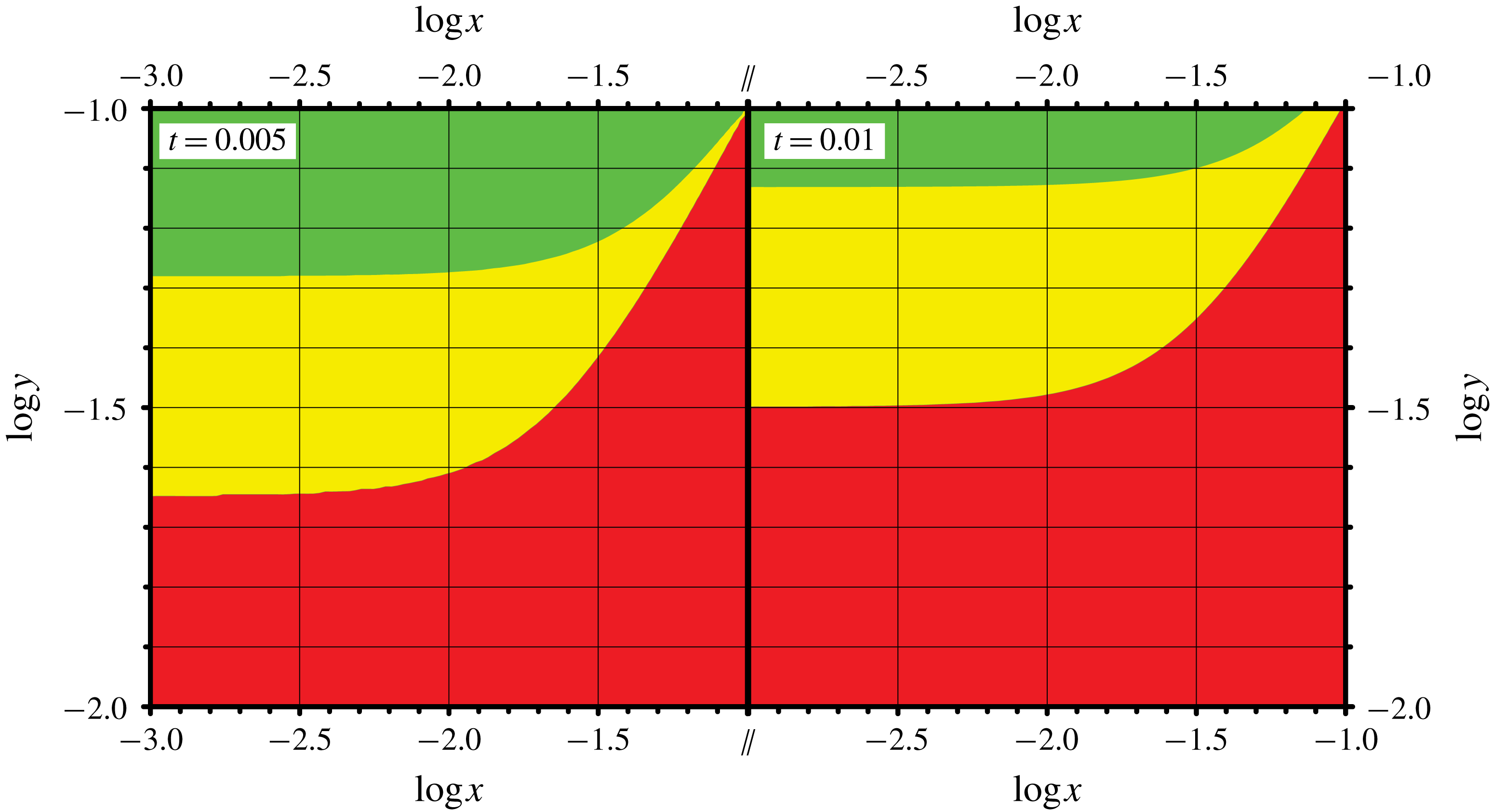
Contour plot of the autocorrelation $\unicode[STIX]{x1D70C}_{H}=C_{H}/\unicode[STIX]{x1D70E}_{H}^{2}$  of the hydraulic head $H$ for $t=0.005$ and $t=0.01$ . Colour legend: $0.95\leqslant \unicode[STIX]{x1D70C}_{H}\leqslant 1$ (red), $0.75\leqslant \unicode[STIX]{x1D70C}_{H}\leqslant 0.95$ (yellow) and $\unicode[STIX]{x1D70C}_{H}\leqslant 0.75$ (green).

In classical applications aiming at the identification of a formation’s properties (Kruseman & de Ridder Reference Kruseman and de Ridder1979) the correlation between head measurements is tacitly ignored. However, such a correlation has a deep impact upon the correct identification of the formation’s parameters. More precisely, in order to identify the hydraulic properties (even when the formation can be regarded as homogeneous) it is instrumental to match the theoretical model against head measurements which are scarcely correlated (see, e.g. discussion in Gómez et al. Reference Gómez, Severino, Randazzo, Toraldo and Otero2009). To this end, we depict in figure 2 the contour plot (with the modulus of the position vectors in $\log$ -scale) of the correlation coefficient $\unicode[STIX]{x1D70C}_{H}=C_{H}/\unicode[STIX]{x1D70E}_{H}^{2}$ of the hydraulic head $H$ pertaining to two parallel positions, for $t=0.005$ and $t=0.01$ . Specifically, figure 2 reads as follows: the head measurements are (i) largely, (ii) moderately or (iii) scarcely correlated when the point $(x,y)$ lies within (i) the red area ( $0.95\leqslant \unicode[STIX]{x1D70C}_{H}\leqslant 1$ ), (ii) the yellow strip ( $0.75\leqslant \unicode[STIX]{x1D70C}_{H}\leqslant 0.95$ ) or (iii) the green area ( $\unicode[STIX]{x1D70C}_{H}\leqslant 0.75$ ). The striking result is that at very early times the regions (green) of scarce correlation are larger as compared with those detected at larger times. Hence, from the identification standpoint it is recommended to carry out most of the sampling at early times. This is true not only for linear flows, but it also applies to nonlinear flows (see, e.g. Severino, Santini & Sommella Reference Severino, Santini and Sommella2003; Severino et al. Reference Severino, Monetti, Santini and Toraldo2006).

3.2 Source of constant strength

We now consider a flow generated by a source of constant strength that, without loss of generality, is assumed unitary. Such a problem is of definite theoretical interest in fluid mechanics since it enables one to investigate the tendency of unsteady flows past a circular obstacle towards steady ones (see, e.g. Milne-Thomson Reference Milne-Thomson1968, ch. 8.61).

Before proceeding further, it is worth discussing briefly how the sampling strategy should be carried out during a pumping test in this case. More precisely, in order to record pressure values that are meaningful for the identification of hydraulic properties, sampling has to be extremely dense before the unsteady regime is exhausted. In fact, under steady-state conditions the medium surrounding the source behaves practically as a homogeneous one (Dagan & Lessoff Reference Dagan and Lessoff2007), therefore rendering meaningless pressure values acquired subsequently. Thus, the knowledge of the decay with time of the head’s fluctuation (see results of § 4.1) combined with the expression of the head variance provided here allows one to design a proper sampling strategy to adopt in classical (i.e.  $Q=\text{const.}$ ) pumping tests at regional scale.

The homogeneous head is

(3.13) $$\begin{eqnarray}H^{(0)}(x,t)=\int _{0}^{t}\frac{\text{d}\unicode[STIX]{x1D70F}}{\unicode[STIX]{x1D70F}}G_{(2)}(x,\unicode[STIX]{x1D70F})=-\frac{1}{4\unicode[STIX]{x03C0}}\text{Ei}\left(-\frac{x^{2}}{4t}\right),\end{eqnarray}$$

and thus the fluctuation (2.8) becomes

(3.14) $$\begin{eqnarray}H^{(1)}(\boldsymbol{x},t)=\frac{1}{4}\int _{0}^{t}\frac{\text{d}\unicode[STIX]{x1D70F}}{t-\unicode[STIX]{x1D70F}}\int _{0}^{\unicode[STIX]{x1D70F}}\frac{\text{d}u}{u}\int _{\unicode[STIX]{x1D6FA}_{2}}\text{d}\bar{\boldsymbol{x}}\unicode[STIX]{x1D700}(\bar{\boldsymbol{x}})G_{(2)}(\bar{x},u)\bar{\boldsymbol{x}}\boldsymbol{\cdot }(\bar{\boldsymbol{x}}-\boldsymbol{x})G_{(2)}(|\bar{\boldsymbol{x}}-\boldsymbol{x}|,t-\unicode[STIX]{x1D70F}).\end{eqnarray}$$

Hence, similarly to the previous section, we write the head covariance as

(3.15) $$\begin{eqnarray}\displaystyle C_{H}(\boldsymbol{x},\boldsymbol{y},t) & = & \displaystyle \frac{\unicode[STIX]{x1D70E}^{2}}{16}\int _{0}^{t}\int _{0}^{t}\text{d}\unicode[STIX]{x1D70F}^{\prime }\text{d}\unicode[STIX]{x1D70F}^{\prime \prime }\frac{G_{(2)}(x,t-\unicode[STIX]{x1D70F}^{\prime })G_{(2)}(y,t-\unicode[STIX]{x1D70F}^{\prime \prime })}{(t-\unicode[STIX]{x1D70F}^{\prime })(t-\unicode[STIX]{x1D70F}^{\prime \prime })}\nonumber\\ \displaystyle & & \displaystyle \times \,\int _{0}^{\unicode[STIX]{x1D70F}^{\prime }}\int _{0}^{\unicode[STIX]{x1D70F}^{\prime \prime }}\frac{\text{d}u\,\text{d}v}{uv}\unicode[STIX]{x1D6F6}_{Q}(a,\unicode[STIX]{x1D6FC};b\boldsymbol{x},\unicode[STIX]{x1D6FD}\boldsymbol{y}),\end{eqnarray}$$

where we have set

(3.16) $$\begin{eqnarray}\displaystyle & & \displaystyle \unicode[STIX]{x1D6F6}_{Q}(a,\unicode[STIX]{x1D6FC};b\boldsymbol{x},\unicode[STIX]{x1D6FD}\boldsymbol{y})=\left(\frac{\unicode[STIX]{x2202}}{\unicode[STIX]{x2202}a}+\frac{\unicode[STIX]{x2202}}{\unicode[STIX]{x2202}b}\right)\left(\frac{\unicode[STIX]{x2202}}{\unicode[STIX]{x2202}\unicode[STIX]{x1D6FC}}+\frac{\unicode[STIX]{x2202}}{\unicode[STIX]{x2202}\unicode[STIX]{x1D6FD}}\right)\int _{\unicode[STIX]{x1D6FA}_{2}}\int _{\unicode[STIX]{x1D6FA}_{2}}\text{d}\bar{\boldsymbol{x}}\,\text{d}\bar{\boldsymbol{y}}\unicode[STIX]{x1D70C}(\bar{\boldsymbol{x}}-\bar{\boldsymbol{y}})\nonumber\\ \displaystyle & & \displaystyle \quad \times \,G_{(2)}(\bar{x},u)G_{(2)}(\bar{y},v)\exp (-a\bar{x}^{2}+b\boldsymbol{x}\boldsymbol{\cdot }\bar{\boldsymbol{x}}-\unicode[STIX]{x1D6FC}\bar{y}^{2}+\unicode[STIX]{x1D6FD}\boldsymbol{y}\boldsymbol{\cdot }\bar{\boldsymbol{y}}).\end{eqnarray}$$

By accounting for (3.3), and carrying out the algebraic derivations, the final result (after changing the order of integration) reads as

(3.17) $$\begin{eqnarray}\displaystyle C_{H}(\boldsymbol{x},\boldsymbol{y},t) & = & \displaystyle \left(\frac{\unicode[STIX]{x1D70E}}{4\unicode[STIX]{x03C0}}\right)^{2}\int _{0}^{t}\int _{0}^{t}\text{d}u\,\text{d}v\int _{0}^{t-u}\int _{0}^{t-v}\frac{\text{d}\unicode[STIX]{x1D70F}^{\prime }\text{d}\unicode[STIX]{x1D70F}^{\prime \prime }}{\mathtt{T}_{Q}^{2}}{\mathcal{C}}_{Q}(u,v,\unicode[STIX]{x1D70F}^{\prime },\unicode[STIX]{x1D70F}^{\prime \prime })\nonumber\\ \displaystyle & & \displaystyle \times \,\exp \left(-\frac{x^{2}t_{Q_{x}}+y^{2}t_{Q_{y}}-8uv\boldsymbol{x}\boldsymbol{\cdot }\boldsymbol{y}}{4\mathtt{T}_{Q}}\right),\end{eqnarray}$$

with

(3.18a,b ) $$\begin{eqnarray}t_{Q_{x}}=v(1+4u)+(1+4u+4v)\unicode[STIX]{x1D70F}^{\prime \prime },\quad t_{Q_{y}}=u(1+4v)+(1+4u+4v)\unicode[STIX]{x1D70F}^{\prime },\end{eqnarray}$$

(3.19) $$\begin{eqnarray}\mathtt{T}_{Q}=uv+v(1+4u)\unicode[STIX]{x1D70F}^{\prime }+(1+4u+4v)\unicode[STIX]{x1D70F}^{\prime }\unicode[STIX]{x1D70F}^{\prime \prime }+u(1+4v)\unicode[STIX]{x1D70F}^{\prime \prime }.\end{eqnarray}$$

The characteristic function ${\mathcal{C}}_{Q}\equiv {\mathcal{C}}_{Q}(u,v,\unicode[STIX]{x1D70F}^{\prime },\unicode[STIX]{x1D70F}^{\prime \prime })$ is

(3.20) $$\begin{eqnarray}\displaystyle & & \displaystyle {\mathcal{C}}_{Q}(u,v,\unicode[STIX]{x1D70F}^{\prime },\unicode[STIX]{x1D70F}^{\prime \prime })\nonumber\\ \displaystyle & & \displaystyle =1+\frac{32}{\mathtt{T}_{Q}}uv\unicode[STIX]{x1D70F}^{\prime }\unicode[STIX]{x1D70F}^{\prime \prime }+\frac{x^{2}}{4\mathtt{T}_{Q}^{2}}[16u^{2}v\unicode[STIX]{x1D70F}^{\prime \prime }(3{\mathcal{T}}_{Q}^{\prime \prime }+16v\unicode[STIX]{x1D70F}^{\prime }\unicode[STIX]{x1D70F}^{\prime \prime })-(1+4u){\mathcal{T}}_{Q}^{\prime }{\mathcal{T}}_{Q}^{\prime \prime 2}]\nonumber\\ \displaystyle & & \displaystyle +\,\frac{y^{2}}{4\mathtt{T}_{Q}^{2}}[16uv^{2}\unicode[STIX]{x1D70F}^{\prime }(3{\mathcal{T}}_{Q}^{\prime }+\!16u\unicode[STIX]{x1D70F}^{\prime }\unicode[STIX]{x1D70F}^{\prime \prime })\!-\!(1\!+\!4v){\mathcal{T}}_{Q}^{\prime 2}{\mathcal{T}}_{Q}^{\prime \prime }]\!+\frac{\boldsymbol{x}\boldsymbol{\cdot }\boldsymbol{y}}{2\mathtt{T}_{Q}^{2}}\{\!{\mathcal{T}}_{Q}^{\prime }{\mathcal{T}}_{Q}^{\prime \prime }[\!{\mathcal{T}}_{Q}^{\prime }{\mathcal{T}}_{Q}^{\prime \prime }-\!4(v{\mathcal{T}}_{Q}^{\prime }+\!u{\mathcal{T}}_{Q}^{\prime \prime })\nonumber\\ \displaystyle & & \displaystyle +\,4uv(3-8\unicode[STIX]{x1D70F}^{\prime }\unicode[STIX]{x1D70F}^{\prime \prime })\!]+\,64uv\unicode[STIX]{x1D70F}^{\prime }\unicode[STIX]{x1D70F}^{\prime \prime }[v{\mathcal{T}}_{Q}^{\prime }+u{\mathcal{T}}_{Q}^{\prime \prime }+uv(1+4\unicode[STIX]{x1D70F}^{\prime }\unicode[STIX]{x1D70F}^{\prime \prime })]\!\}+\frac{x^{4}}{\mathtt{T}_{Q}^{3}}u^{2}v\unicode[STIX]{x1D70F}^{\prime \prime }{\mathcal{T}}_{Q}^{\prime \prime }[\!16uv\unicode[STIX]{x1D70F}^{\prime \prime }\nonumber\\ \displaystyle & & \displaystyle -\,(1+4u){\mathcal{T}}_{Q}^{\prime \prime }\!]+\frac{y^{4}}{\mathtt{T}_{Q}^{3}}uv^{2}\unicode[STIX]{x1D70F}^{\prime }{\mathcal{T}}_{Q}^{\prime }[16uv\unicode[STIX]{x1D70F}^{\prime }-(1+4v){\mathcal{T}}_{Q}^{\prime }]+(\boldsymbol{x}\boldsymbol{\cdot }\boldsymbol{y})^{2}\frac{uv}{\mathtt{T}_{Q}^{3}} [\!{\mathcal{T}}_{Q}^{\prime }({\mathcal{T}}_{Q}^{\prime \prime }-2v)\nonumber\\ \displaystyle & & \displaystyle -\,16uv\unicode[STIX]{x1D70F}^{\prime }\unicode[STIX]{x1D70F}^{\prime \prime }\!][{\mathcal{T}}_{Q}^{\prime \prime }({\mathcal{T}}_{Q}^{\prime }-2u)-16uv\unicode[STIX]{x1D70F}^{\prime }\unicode[STIX]{x1D70F}^{\prime \prime }]+x^{2}\boldsymbol{x}\boldsymbol{\cdot }\boldsymbol{y}\frac{u}{4\mathtt{T}_{Q}^{2}}\left\{16uv^{2}\unicode[STIX]{x1D70F}^{\prime \prime }\left(\frac{2u}{\mathtt{T}_{Q}}{\mathcal{T}}_{Q}^{\prime \prime }-1\right)+{\mathcal{T}}_{Q}^{\prime \prime }\right.\nonumber\\ \displaystyle & & \displaystyle \times \left.[(1+4u){\mathcal{T}}_{Q}^{\prime \prime }-16uv\unicode[STIX]{x1D70F}^{\prime \prime }]-\frac{2v}{\mathtt{T}_{Q}}{\mathcal{T}}_{Q}^{\prime }{\mathcal{T}}_{Q}^{\prime \prime }[{\mathcal{T}}_{Q}^{\prime \prime }+4u(v+\unicode[STIX]{x1D70F}^{\prime \prime })]\right\}+y^{2}\boldsymbol{x}\boldsymbol{\cdot }\boldsymbol{y}\frac{v}{4\mathtt{T}_{Q}^{2}}\left\{16u^{2}v\unicode[STIX]{x1D70F}^{\prime }\right.\nonumber\\ \displaystyle & & \displaystyle \times \left.\left(\frac{2v}{\mathtt{T}_{Q}}{\mathcal{T}}_{Q}^{\prime }-1\right)+{\mathcal{T}}_{Q}^{\prime }[(1+4v){\mathcal{T}}_{Q}^{\prime }-16uv\unicode[STIX]{x1D70F}^{\prime }]-\frac{2u}{\mathtt{T}_{Q}}{\mathcal{T}}_{Q}^{\prime }{\mathcal{T}}_{Q}^{\prime \prime }[{\mathcal{T}}_{Q}^{\prime }+4v(u+\unicode[STIX]{x1D70F}^{\prime })]\right\},\nonumber\\ \displaystyle & & \displaystyle\end{eqnarray}$$

where

(3.21a,b ) $$\begin{eqnarray}{\mathcal{T}}_{Q}^{\prime }=u+(1+4u)\unicode[STIX]{x1D70F}^{\prime },\quad {\mathcal{T}}_{Q}^{\prime \prime }=v+(1+4v)\unicode[STIX]{x1D70F}^{\prime \prime }.\end{eqnarray}$$

It is seen that to compute the head covariance (3.17) it suffices to carry out four quadratures. This represents a reduction of the required computational burden even as compared with the steady version of the same problem (Riva et al. Reference Riva, Guadagnini, Neuman and Franzetti2001). The head covariance (3.17) is a robust tool to design pressure monitoring to be used in the analysis of pumping tests (Fallico et al. Reference Fallico, De Bartolo, Veltri and Severino2016, Reference Fallico, Ianchello, De Bartolo and Severino2018).

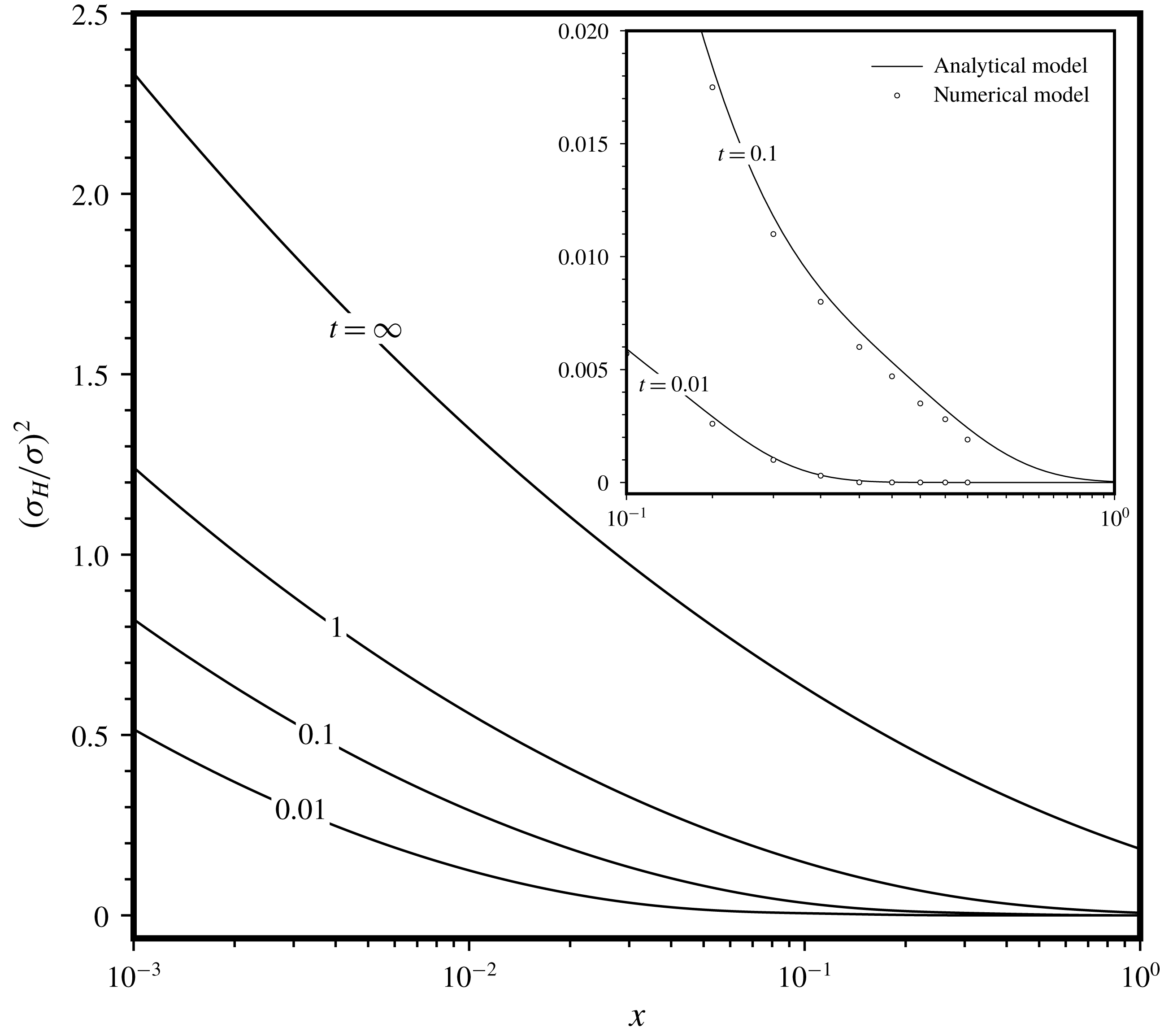
In order to show how the uncertainty affects the hydraulic head, in figure 3 we depict the scaled variance $\unicode[STIX]{x1D70E}_{H}^{2}/\unicode[STIX]{x1D70E}^{2}$ versus the distance $x$ and a few values of the time  $t$ . For comparison purposes, we have also produced Monte Carlo simulations. For the sake of completeness, we briefly describe the algorithm herein. Thus, any realization of the random field $K$ is mapped upon a square mesh (step I) with denser nodal distribution around the source. Then, the parabolic equation (1.4) with $\unicode[STIX]{x1D719}\equiv \unicode[STIX]{x1D6FF}(\boldsymbol{x})$ is discretized (finite difference method) into a system of algebraic equations which is solved for the nodal $H$ values (step II). Steps I–II are iterated ( ${\mathcal{N}}=10^{4}$ ) to obtain at each node a set of $H$ realizations which are used to compute $\unicode[STIX]{x1D70E}_{H}^{2}$ .

Figure 3.

Dependence of the scaled variance $(\unicode[STIX]{x1D70E}_{H}/\unicode[STIX]{x1D70E})^{2}$ of the hydraulic head upon the modulus $x$ of the distance from the source, and some values of the dimensionless time  $t$ . The insert shows a comparison of the analytical (continuous line) against the numerical (symbol) model in the range $x\in [0.1;1.0]$ for $t=0.01$ and $t=0.1$ .

At first glance, it is seen that the variance $\unicode[STIX]{x1D70E}_{H}^{2}$ is singular at the source. This is explained by recalling that surrounding the source the flow domain can be homogenized by means of the harmonic conductivity $K_{H}$ (see discussion in the previous section). Hence, due to the singular nature of the homogeneous head (3.13), the same behaviour is detected for the variance. In addition, the reduction of the argument in (3.13) increases with increasing time, and concurrently the variance is larger (for given $x$ ) for longer times. As a consequence, the maximum uncertainty at the source is detected in the long-time regime (in agreement with Dagan Reference Dagan1982). It is worth noting that the numerical simulations (insert in figure 3) are found in good agreement with the analytical results, although they are limited to the early times. This is due to the fact that accounting for longer times would have required a discretization of a very large flow domain, thus leading to an extremely large number of numerical nodes. This further underpins the need and utility (in view of applications) of simple (i.e. analytical) results. From the mechanical standpoint, the behaviour of $\unicode[STIX]{x1D70E}_{H}^{2}$ close to the source has a straightforward explanation. Indeed, we can focus on the pattern of the steady flow as determined by a single inclusion $\unicode[STIX]{x1D6FA}_{0}$ of conductivity $K_{0}$ near the source and embedded into a matrix $\unicode[STIX]{x1D6FA}_{eff}$ of effective conductivity $K_{eff}$ (the head variance being evaluated as ensemble average of the square of the fluctuation $H^{(1)}=H-H^{(0)}$ computed over many such realizations). The exact solution of a steady flow towards a source of constant strength in the presence of a circular inclusion (resembling the statistical structure of an isotropic porous formation, Jankovic, Fiori & Dagan Reference Jankovic, Fiori and Dagan2003) submerged into a matrix of different conductivity was originally derived by Wheatcraft & Winterberg (Reference Wheatcraft and Winterberg1985), and recently generalized by Severino (Reference Severino2019) to account for any position of the centre of the inclusion.

Figure 4.

Contour plot of the hydraulic head (red dashed lines) and stream function (blue continuous lines) as affected by a circular inclusion $\unicode[STIX]{x1D6FA}_{0}$ of conductivity $K_{0}$ implanted close to the source into a matrix $\unicode[STIX]{x1D6FA}_{eff}$ of effective conductivity $K_{eff}$ . The left-hand side refers to a relatively poorly conducting (i.e.  $\unicode[STIX]{x1D705}=K_{0}/K_{eff}\ll 1$ ) inclusion $\unicode[STIX]{x1D6FA}_{0}$ , whereas the right-hand side pertains to the reverse case (i.e.  $\unicode[STIX]{x1D705}=K_{0}/K_{eff}\gg 1$ ).

Thus, in figure 4 we depict a circular inclusion $\unicode[STIX]{x1D6FA}_{0}$ near to the source $\boldsymbol{x}\equiv \left(0,0\right)$ for two largely different values of the ‘contrast ratio’ $\unicode[STIX]{x1D705}\equiv K_{0}/K_{eff}$ . Due to the mass conservation law, the streamlines circumvent the inclusion for $\unicode[STIX]{x1D705}<1$ , and they are attracted by the inclusion (similarly to the channelling mechanism, Fiori & Jankovic Reference Fiori and Jankovic2012; Floryan Reference Floryan2015) for $\unicode[STIX]{x1D705}>1$ . The resulting deformation of the streamlines in the vicinity of the inclusion determines steeper gradients above/below it, and consequently the hydraulic head in the close vicinity of the inclusion is higher ( $\unicode[STIX]{x1D705}<1$ ) or lower ( $\unicode[STIX]{x1D705}>1$ ) than the mean $H^{(0)}$ . As a consequence, in both cases the variance $\unicode[STIX]{x1D70E}_{H}^{2}\equiv \langle H^{(1)2}\rangle$ increases. Away from the source, the head variance reduces since the conditioning effect due to the source becomes immaterial. Nevertheless, it has to be noted that in the far field the mean head $H^{(0)}$ also decays (see (3.13)), and therefore one cannot claim that the relative uncertainty $\unicode[STIX]{x1D70E}_{H}/H^{(0)}$ does. This explains why in practical applications monitoring of the pressure is not recommended to be carried out far from the source. Finally, it is worth noting that, although such a mechanical picture applies rigorously to steady flows, it nevertheless enables one to draw the same conclusions under transient conditions, the variance $\unicode[STIX]{x1D70E}_{H}^{2}$ being in this case just reduced by a factor proportional to the time.

4 Flow at formation scale $(d=3)$

We are concerned here with the computation of the head covariance for a flow driven by sources distributed along a line. Such a configuration is typical of pumping tests in three-dimensional porous formations. In fact, for a well radius $r_{w}$ much smaller than $\ell$ , a condition which is frequently met since $r_{w}\simeq O(\text{cm})$ and $\ell \simeq O(\text{m})$ , one can replace the well by a singular line, i.e.  $\unicode[STIX]{x1D719}\equiv \unicode[STIX]{x1D6FF}(\boldsymbol{x}_{r})\unicode[STIX]{x1D6FF}(t)$ (Indelman Reference Indelman2003).

To compute the covariance in this case, it was found more convenient from the mathematical point of view to start directly from the fluctuation (2.7) that, for a singular line, is written as follows:

(4.1) $$\begin{eqnarray}\displaystyle & \displaystyle H^{(1)}(\boldsymbol{x},t)=\frac{1}{4(4\unicode[STIX]{x03C0})^{5/2}}\int _{0}^{t}\frac{\text{d}\unicode[STIX]{x1D70F}^{\prime }}{\unicode[STIX]{x1D70F}^{\prime 2}(t-\unicode[STIX]{x1D70F}^{\prime })^{5/2}}\exp \left[-\frac{x_{r}^{2}}{4(t-\unicode[STIX]{x1D70F}^{\prime })}\right]\unicode[STIX]{x1D6F6}(\boldsymbol{x},a,b), & \displaystyle\end{eqnarray}$$

(4.2) $$\begin{eqnarray}\displaystyle & \displaystyle \unicode[STIX]{x1D6F6}(\boldsymbol{x},a,b)=\int _{\unicode[STIX]{x1D6FA}_{3}}\text{d}\bar{\boldsymbol{x}}\exp \left[-\frac{(x_{3}-\bar{x}_{3})^{2}}{4(t-\unicode[STIX]{x1D70F}^{\prime })}\right]\bar{\boldsymbol{x}}_{r}\boldsymbol{\cdot }(\boldsymbol{x}_{r}-\bar{\boldsymbol{x}}_{r})\exp (-a\bar{x}_{r}^{2}+b\boldsymbol{x}_{r}\boldsymbol{\cdot }\bar{\boldsymbol{x}}_{r})\unicode[STIX]{x1D700}(\bar{\boldsymbol{x}}).\qquad & \displaystyle\end{eqnarray}$$

Note that in this case the leading-order term $H^{(0)}(x_{r},t)=G_{(2)}(x_{r},t)$ has been obtained by integrating the Green function pertaining to $d=3$ over the vertical coordinate. Hence, the head covariance $C_{H}(\boldsymbol{x},\boldsymbol{y},t)$ is written as

(4.3) $$\begin{eqnarray}\displaystyle C_{H}(\boldsymbol{x},\boldsymbol{y},t) & = & \displaystyle \frac{1}{4(4\unicode[STIX]{x03C0})^{5/2}}\int _{0}^{t}\frac{\text{d}\unicode[STIX]{x1D70F}^{\prime }}{\unicode[STIX]{x1D70F}^{\prime 2}(t-\unicode[STIX]{x1D70F}^{\prime })^{5/2}}\exp \left[-\frac{x_{r}^{2}}{4(t-\unicode[STIX]{x1D70F}^{\prime })}\right]\int _{\unicode[STIX]{x1D6FA}_{3}}\text{d}\bar{\boldsymbol{x}}\exp \left[-\frac{(x_{3}-\bar{x}_{3})^{2}}{4(t-\unicode[STIX]{x1D70F}^{\prime })}\right]\nonumber\\ \displaystyle & & \displaystyle \quad \times \,\bar{\boldsymbol{x}}_{r}\boldsymbol{\cdot }(\bar{\boldsymbol{x}}_{r}-\boldsymbol{x}_{r})\exp (-a\bar{x}_{r}^{2}+b\boldsymbol{x}_{r}\boldsymbol{\cdot }\bar{\boldsymbol{x}}_{r})C_{\unicode[STIX]{x1D700}H}(\bar{\boldsymbol{x}},\boldsymbol{y},t),\end{eqnarray}$$

where the cross-covariance $C_{\unicode[STIX]{x1D700}H}(\boldsymbol{x},\boldsymbol{y},t)=\langle \unicode[STIX]{x1D700}(\boldsymbol{x})H^{(1)}(\boldsymbol{y},t)\rangle$ is

(4.4) $$\begin{eqnarray}\displaystyle C_{\unicode[STIX]{x1D700}H}(\boldsymbol{x},\boldsymbol{y},t) & = & \displaystyle \frac{\unicode[STIX]{x1D70E}^{2}}{4(4\unicode[STIX]{x03C0})^{5/2}}\int _{0}^{t}\frac{\text{d}\unicode[STIX]{x1D70F}^{\prime }}{\unicode[STIX]{x1D70F}^{\prime 2}(t-\unicode[STIX]{x1D70F}^{\prime })^{5/2}}\exp \left[-\frac{y_{r}^{2}}{4(t-\unicode[STIX]{x1D70F}^{\prime })}\right]\int _{\unicode[STIX]{x1D6FA}_{3}}\text{d}\bar{\boldsymbol{y}}\exp \left[-\frac{(y_{3}-\bar{y}_{3})^{2}}{4(t-\unicode[STIX]{x1D70F}^{\prime })}\right]\nonumber\\ \displaystyle & & \displaystyle \times \,\bar{\boldsymbol{y}}_{r}\boldsymbol{\cdot }(\boldsymbol{y}_{r}-\bar{\boldsymbol{y}}_{r})\exp (-a\bar{y}_{r}^{2}+b\boldsymbol{y}_{r}\boldsymbol{\cdot }\bar{\boldsymbol{y}}_{r})\unicode[STIX]{x1D70C}(\boldsymbol{x}-\bar{\boldsymbol{y}}).\end{eqnarray}$$

Before proceeding further, we note that at formation scale the Gaussian autocorrelation $\unicode[STIX]{x1D70C}$ (with lengths divided by the horizontal integral scale $\ell$ ) has an axisymmetric structure, i.e.

(4.5) $$\begin{eqnarray}\unicode[STIX]{x1D70C}(\boldsymbol{x})\equiv \exp \left[-x_{r}^{2}-\left(\frac{x_{3}}{\unicode[STIX]{x1D706}}\right)^{2}\right],\end{eqnarray}$$

where $\boldsymbol{x}_{r}\equiv (x_{1},x_{2})$ is the position in the horizontal plane and $x_{3}$ is the coordinate along the axis of anisotropy. The dimensionless parameter $\unicode[STIX]{x1D706}\in ]0;1\!]$ is the anisotropy ratio (Dagan Reference Dagan1989).

We concentrate hereafter on the explicit derivation of the head variance $\unicode[STIX]{x1D70E}_{H}^{2}$ . In order to compute the cross-covariance $C_{\unicode[STIX]{x1D700}H}$ , we note preliminarily that the inner (spatial) quadratures appearing in (4.4) can be analytically carried out, i.e.

(4.6) $$\begin{eqnarray}\displaystyle & & \displaystyle \int _{\unicode[STIX]{x1D6FA}_{3}}\text{d}\bar{\boldsymbol{y}}\exp \left[-\frac{(y_{3}-\bar{y}_{3})^{2}}{4(t-\unicode[STIX]{x1D70F}^{\prime })}\right]\bar{\boldsymbol{y}}_{r}\boldsymbol{\cdot }(\boldsymbol{y}_{r}-\bar{\boldsymbol{y}}_{r})\exp (-a\bar{y}_{r}^{2}+b\boldsymbol{y}_{r}\boldsymbol{\cdot }\bar{\boldsymbol{y}}_{r})\unicode[STIX]{x1D70C}(\boldsymbol{x}-\bar{\boldsymbol{y}})\nonumber\\ \displaystyle & & \displaystyle =\int _{-\infty }^{+\infty }\text{d}\bar{y}_{3}\exp \left[-\frac{(y_{3}-\bar{y}_{3})^{2}}{4(t-\unicode[STIX]{x1D70F}^{\prime })}-\left(\frac{x_{3}-\bar{y}_{3}}{\unicode[STIX]{x1D706}}\right)^{2}\right]\nonumber\\ \displaystyle & & \displaystyle \times \,\int _{\unicode[STIX]{x1D6FA}_{2}}\text{d}\bar{\boldsymbol{y}}_{r}\,\bar{\boldsymbol{y}}_{r}\boldsymbol{\cdot }(\boldsymbol{y}_{r}-\bar{\boldsymbol{y}}_{r})\exp (-a\bar{y}_{r}^{2}+b\boldsymbol{y}_{r}\boldsymbol{\cdot }\bar{\boldsymbol{y}}_{r})\exp (-|\boldsymbol{x}_{r}-\bar{\boldsymbol{y}}_{r}|^{2})=2\unicode[STIX]{x1D706}\sqrt{\frac{\unicode[STIX]{x03C0}(t-\unicode[STIX]{x1D70F}^{\prime })}{\unicode[STIX]{x1D706}^{2}+4(t-\unicode[STIX]{x1D70F}^{\prime })}}\nonumber\\ \displaystyle & & \displaystyle \times \,\exp \left[-\frac{(x_{3}-y_{3})^{2}}{\unicode[STIX]{x1D706}^{2}+4(t-\unicode[STIX]{x1D70F}^{\prime })}\right]\left(\frac{\unicode[STIX]{x2202}}{\unicode[STIX]{x2202}a}+\frac{\unicode[STIX]{x2202}}{\unicode[STIX]{x2202}b}\right)\int _{\unicode[STIX]{x1D6FA}_{2}}\text{d}\bar{\boldsymbol{y}}_{r}\exp (-a\bar{y}_{r}^{2}+b\boldsymbol{y}_{r}\boldsymbol{\cdot }\bar{\boldsymbol{y}}_{r})\exp (-|\boldsymbol{x}_{r}-\bar{\boldsymbol{y}}_{r}|^{2}).\nonumber\\ \displaystyle & & \displaystyle\end{eqnarray}$$

Then, by noting that

(4.7) $$\begin{eqnarray}\displaystyle & & \displaystyle \int _{\unicode[STIX]{x1D6FA}_{2}}\text{d}\bar{\boldsymbol{y}}_{r}\exp (-a\bar{y}_{r}^{2}+b\boldsymbol{y}_{r}\boldsymbol{\cdot }\bar{\boldsymbol{y}}_{r})\exp (-|\boldsymbol{x}_{r}-\bar{\boldsymbol{y}}_{r}|^{2})=\frac{\unicode[STIX]{x03C0}}{1+a}\exp \left(-\frac{ax_{r}^{2}}{1+a}\right)\nonumber\\ \displaystyle & & \displaystyle \quad \times \,\exp \left[\frac{b^{2}y_{r}^{2}}{4(1+a)}+b\frac{\boldsymbol{x}_{r}\boldsymbol{\cdot }\boldsymbol{y}_{r}}{1+a}\right],\end{eqnarray}$$

and back substitution into (4.4) leads (after carrying out the required differentiations with respect to the fictitious variables $a$ and $b$ ) to

(4.8) $$\begin{eqnarray}C_{\unicode[STIX]{x1D700}H}=\frac{\unicode[STIX]{x1D706}}{4\unicode[STIX]{x03C0}}\unicode[STIX]{x1D70E}^{2}\int _{0}^{t}\text{d}\unicode[STIX]{x1D70F}\frac{\overline{{\mathcal{C}}}_{\unicode[STIX]{x1D700}H}(t,\unicode[STIX]{x1D70F})}{T_{t}^{3}T_{\unicode[STIX]{x1D706}^{2}}^{1/2}}\exp \left[-\frac{(x_{3}-y_{3})^{2}}{T_{\unicode[STIX]{x1D706}^{2}}}\right]\exp \left(-\frac{t}{T_{t}}x_{r}^{2}-\frac{1+4\unicode[STIX]{x1D70F}}{4T_{t}}y_{r}^{2}+2\frac{\unicode[STIX]{x1D70F}}{T_{t}}\boldsymbol{x}_{r}\boldsymbol{\cdot }\boldsymbol{y}_{r}\right),\end{eqnarray}$$

where

(4.9a,b ) $$\begin{eqnarray}\overline{{\mathcal{C}}}_{\unicode[STIX]{x1D700}H}(t,\unicode[STIX]{x1D70F})=T_{t}+4\unicode[STIX]{x1D70F}(t-\unicode[STIX]{x1D70F})x_{r}^{2}-\frac{1+4\unicode[STIX]{x1D70F}}{4}y_{r}^{2}+(2\unicode[STIX]{x1D70F}-T_{t})\boldsymbol{x}_{r}\boldsymbol{\cdot }\boldsymbol{y}_{r},\quad T_{\unicode[STIX]{x1D6FC}}=\unicode[STIX]{x1D6FC}+4\unicode[STIX]{x1D70F}(t-\unicode[STIX]{x1D70F}).\end{eqnarray}$$

Finally, insertion of (4.8)–(4.9) into (4.3) leads (after computing one spatial quadrature) to

(4.10) $$\begin{eqnarray}\displaystyle & & \displaystyle \unicode[STIX]{x1D70E}_{H}^{2}(\boldsymbol{x}_{r},t)=\frac{\unicode[STIX]{x1D706}\unicode[STIX]{x1D70E}^{2}}{256\unicode[STIX]{x03C0}^{3}}\int _{0}^{t}\frac{\text{d}\unicode[STIX]{x1D70F}^{\prime }}{[(t-\unicode[STIX]{x1D70F}^{\prime })\unicode[STIX]{x1D70F}^{\prime }]^{2}}\exp \left[-\frac{x_{r}^{2}}{4(t-\unicode[STIX]{x1D70F}^{\prime })}\right]\int _{0}^{t}\frac{\text{d}\unicode[STIX]{x1D70F}^{\prime \prime }}{{\mathcal{T}}_{\unicode[STIX]{x1D706}}^{1/2}{\mathcal{T}}^{\prime \prime 3}}\int _{\unicode[STIX]{x1D6FA}_{2}}\text{d}\bar{\boldsymbol{x}}_{r}\overline{{\mathcal{C}}}_{\unicode[STIX]{x1D700}H}(t,\unicode[STIX]{x1D70F}^{\prime \prime })\nonumber\\ \displaystyle & & \displaystyle \times \,\bar{\boldsymbol{x}}_{r}\boldsymbol{\cdot }(\bar{\boldsymbol{x}}_{r}-\boldsymbol{x}_{r})\exp (-a\bar{x}_{r}^{2}+b\boldsymbol{x}_{r}\boldsymbol{\cdot }\bar{\boldsymbol{x}}_{r})\exp \left(-\frac{t\bar{x}_{r}^{2}}{{\mathcal{T}}^{\prime \prime }}-\frac{1+4\unicode[STIX]{x1D70F}^{\prime \prime }}{4{\mathcal{T}}^{\prime \prime }}x_{r}^{2}+2\frac{\unicode[STIX]{x1D70F}^{\prime \prime }}{{\mathcal{T}}^{\prime \prime }}\bar{\boldsymbol{x}}_{r}\boldsymbol{\cdot }\boldsymbol{x}_{r}\right),\end{eqnarray}$$

where we have set ${\mathcal{T}}_{\unicode[STIX]{x1D706}}=\unicode[STIX]{x1D706}^{2}+4[t-\unicode[STIX]{x1D70F}^{\prime }+(t-\unicode[STIX]{x1D70F}^{\prime \prime })\unicode[STIX]{x1D70F}^{\prime \prime }]$ and ${\mathcal{T}}^{\prime \prime }=t+4(t-\unicode[STIX]{x1D70F}^{\prime \prime })\unicode[STIX]{x1D70F}^{\prime \prime }$ . Overall, the head variance (4.10) is expressed by means of four quadratures. In particular, it is seen that $\unicode[STIX]{x1D70E}_{H}^{2}$ depends only upon the horizontal coordinate $\boldsymbol{x}_{r}$ . This is explained by recalling that the leading-order term $H^{(0)}$ does not depend upon the vertical coordinate $x_{3}$ , and concurrently the various (cross-)variances of the flow variables become stationary along $x_{3}$ .

Figure 5.

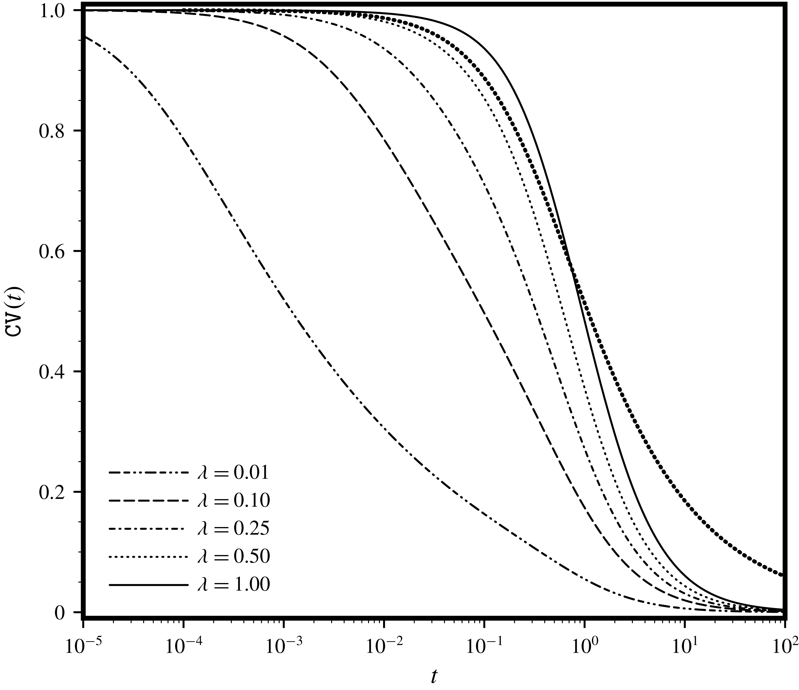
Dependence of the scaled coefficient of variation $\mathtt{CV}(t)$ along the well as a function of the dimensionless time $t$ , and for several values of the anisotropy ratio. The dotted (thick) line refers to the same expression of CV at regional ( $d=2$ ) scale.

To grasp the behaviour of the head variance by a simple expression, we focus on the pattern of (4.10) along a very tiny annulus (i.e.  $x_{r}\ll 1$ ) surrounding the well. In this case, evaluation of $\unicode[STIX]{x1D70E}_{H}^{2}$ is reduced (we omit the cumbersome algebraic derivations) to two quadratures solely, the final result being

(4.11) $$\begin{eqnarray}\unicode[STIX]{x1D70E}_{H}^{2}\simeq \unicode[STIX]{x1D706}\unicode[STIX]{x1D70E}^{2}H^{(0)2}(0,t)\int _{0}^{t}\int _{0}^{t}\frac{\text{d}\unicode[STIX]{x1D70F}^{\prime }\,\text{d}\unicode[STIX]{x1D70F}^{\prime \prime }}{\mathtt{T}^{2}{\mathcal{T}}_{\unicode[STIX]{x1D706}}^{1/2}}\left[1+\frac{32}{t\mathtt{T}}\unicode[STIX]{x1D70F}^{\prime }(t-\unicode[STIX]{x1D70F}^{\prime })(t-\unicode[STIX]{x1D70F}^{\prime \prime })\right].\end{eqnarray}$$

In figure 5 we depict the scaled coefficient of variation $\mathtt{CV}(t)\equiv \unicode[STIX]{x1D70E}_{H}/(\unicode[STIX]{x1D70E}H^{(0)}(0,t))$ as a function of the dimensionless time $t$ , and for several values of the anisotropy ratio $\unicode[STIX]{x1D706}$ . In the initial stage one has $\mathtt{CV}\sim 1$ , which is tantamount to stating that the uncertainty in the head measurements along the well is of the same order of magnitude as the leading-order term $H^{(0)}$ . The decrease of $\mathtt{CV}$ with increasing time enhances with smaller values of the anisotropy ratio $\unicode[STIX]{x1D706}$ . This is explained by noting that the reduction of $\mathtt{CV}$ due to the anisotropy is driven by the quantity $(\unicode[STIX]{x1D706}/t)^{2}$ (see the quantity ${\mathcal{T}}_{\unicode[STIX]{x1D706}}$ in (4.11)), and therefore small $\unicode[STIX]{x1D706}$ values produce the same effect detected in the long-time regime. For comparison purposes, in figure 5 we depict the same CV as computed at regional scale. Note that for isotropic media the difference between the behaviour at regional scale and formation scale is different whether $t$ is less or greater than $1$ . This result should serve as a warning against straightforward extrapolation from lower to higher dimensions in the analysis of pumping tests.

To conclude the present section, we discuss how the general expression (4.1) can be used to tackle different scenarios which are frequently encountered in applications at formation scale. The simplest conceivable case is that of a semi-bounded domain. In this case, the fluctuation is obtained by reflection of the Green function across the boundary (method of images). Extension to a fully penetrating well into an aquifer of finite thickness is achieved likewise (by multiple reflections). Also relevant is the case of a well of finite length $\unicode[STIX]{x1D6E5}$ , which is accounted for by replacing $\unicode[STIX]{x1D719}\rightarrow [\unicode[STIX]{x1D6E9}(x_{3}+\unicode[STIX]{x1D6E5}/2)-\unicode[STIX]{x1D6E9}(x_{3}-\unicode[STIX]{x1D6E5}/2)]\unicode[STIX]{x1D6FF}(\boldsymbol{x}_{r})\unicode[STIX]{x1D6FF}(t)$ ( $\unicode[STIX]{x1D6E9}$ being the Heaviside step function). Besides these configurations of the flow domain, different regimes in the pumping volumetric rate $Q$ can also be considered. In fact, one can deal with: (i) $Q=\text{const.}$ , by integrating the source-line distribution over the time, i.e.  $\unicode[STIX]{x1D719}\rightarrow \unicode[STIX]{x1D6FF}(\boldsymbol{x}_{r})$ , and (ii) a pumping with oscillatory $Q$ (by implementing the procedure of Dagan & Rabinovich Reference Dagan and Rabinovich2014). Another important case pertains to the computation of the head’s fluctuation that ensures a uniform head distribution along the well. It is indeed obtained by supplementing the fluctuation (4.1) with a $\unicode[STIX]{x1D700}$ -order term such that $H^{(1)}$ vanishes for $x_{r}\rightarrow 0$ (for details, see Indelman Reference Indelman2003). Finally, one can superimpose a groundwater (background) flow to delineate the so-called ‘well-capture zone’ as affected by the heterogeneity of the hydraulic conductivity. Before concluding, it is worth recalling that all the above extensions are possible thanks to the linearity of the flow equation and of the boundary condition(s) (superposition principle).

4.1 Analysis of the large time regime

We wish now to investigate the large time behaviour of the head covariance (3.15). More precisely, we prove that in the limit $t\rightarrow \infty$ the head covariance tends to its steady-state expression. This is not a trivial point, since in the asymptotic expansion (2.4) there is no a priori guarantee that the $\unicode[STIX]{x1D70E}^{2}$ -order approximation of the unsteady head covariance will converge to its steady-state expression in the long-time limit. For the sake of generality, we deal with a source flow of any dimensionality $d$ .

Thus, we derive the head fluctuation $H_{w}^{(1)}$ generated by a point source of unit discharge as $H_{w}^{(1)}(\boldsymbol{x},t)=\int _{0}^{t}\text{d}\unicode[STIX]{x1D70F}H^{(1)}(\boldsymbol{x},\unicode[STIX]{x1D70F})$ , $H^{(1)}$ being obtained from (2.8) for $H^{(0)}\equiv G_{(d)}$ , i.e.

(4.12) $$\begin{eqnarray}H_{w}^{(1)}(\boldsymbol{x},t)=\frac{1}{4}\int _{0}^{t}\int _{0}^{\unicode[STIX]{x1D70F}^{\prime }}\int _{\unicode[STIX]{x1D6FA}_{d}}\frac{\text{d}\unicode[STIX]{x1D70F}^{\prime }\,\text{d}\unicode[STIX]{x1D70F}^{\prime \prime }\,\text{d}\bar{\boldsymbol{x}}}{\unicode[STIX]{x1D70F}^{\prime \prime }(\unicode[STIX]{x1D70F}^{\prime }-\unicode[STIX]{x1D70F}^{\prime \prime })}\unicode[STIX]{x1D700}(\bar{\boldsymbol{x}})\bar{\boldsymbol{x}}\boldsymbol{\cdot }(\bar{\boldsymbol{x}}-\boldsymbol{x})G_{(d)}(\bar{x},\unicode[STIX]{x1D70F}^{\prime })G_{(d)}(|\bar{\boldsymbol{x}}-\boldsymbol{x}|,\unicode[STIX]{x1D70F}^{\prime }-\unicode[STIX]{x1D70F}^{\prime \prime }),\end{eqnarray}$$

which is rewritten as

(4.13) $$\begin{eqnarray}H_{w}^{(1)}(\boldsymbol{x},t)=\frac{1}{4}\int _{\unicode[STIX]{x1D6FA}_{d}}\text{d}\bar{\boldsymbol{x}}\unicode[STIX]{x1D700}(\bar{\boldsymbol{x}})\bar{\boldsymbol{x}}\boldsymbol{\cdot }(\bar{\boldsymbol{x}}-\boldsymbol{x})\int _{0}^{t}\frac{\text{d}\unicode[STIX]{x1D70F}}{\unicode[STIX]{x1D70F}}G_{(d)}(|\bar{\boldsymbol{x}}-\boldsymbol{x}|,\unicode[STIX]{x1D70F})\int _{0}^{t-\unicode[STIX]{x1D70F}}\frac{\text{d}u}{u}G_{(d)}(\bar{x},u).\end{eqnarray}$$

The analytical expression $H_{w}^{(1)}(\boldsymbol{x},\infty )$ of the steady-state fluctuation can be computed by means of the large time (Tauber) theorem, i.e.  $H_{w}^{(1)}(\boldsymbol{x},\infty )=\lim _{s\rightarrow 0}s\overline{H}_{w}^{(1)}(\boldsymbol{x},s)$ , where $\overline{H}_{w}^{(1)}(\boldsymbol{x},s)$ is the Laplace transform of (4.13). This latter is straightforwardly derived by means of convolution as

(4.14) $$\begin{eqnarray}\displaystyle & \displaystyle \overline{H}_{w}^{(1)}(\boldsymbol{x},s)=\frac{1}{4}\int _{\unicode[STIX]{x1D6FA}_{d}}\text{d}\bar{\boldsymbol{x}}\unicode[STIX]{x1D700}(\bar{\boldsymbol{x}})\bar{\boldsymbol{x}}\boldsymbol{\cdot }(\bar{\boldsymbol{x}}-\boldsymbol{x})\mathtt{LT}[t^{-1}G_{(d)}(|\boldsymbol{x}-\bar{\boldsymbol{x}}|,t)]s^{-1}\mathtt{LT}[t^{-1}G_{(d)}(\bar{x},t)],\qquad & \displaystyle\end{eqnarray}$$

(4.15) $$\begin{eqnarray}\displaystyle & \displaystyle \mathtt{LT}[t^{-1}G_{(d)}(x,t)]\equiv \frac{1}{2^{d-2}\unicode[STIX]{x03C0}x^{2d-3}}\left\{\begin{array}{@{}ll@{}}\sqrt{s}\text{K}_{1}(x\sqrt{s})\quad & d=2\\ (1+x\sqrt{s})\exp (-x\sqrt{s})\quad & d=3,\end{array}\right. & \displaystyle\end{eqnarray}$$

where $\text{K}_{\unicode[STIX]{x1D708}}(\cdot )$ is the $\unicode[STIX]{x1D708}$ -order modified Bessel function of the second kind (Abramowitz & Stegun Reference Abramowitz and Stegun1972). Besides the large time value, it is also important to estimate the rate of approaching such an asymptotic. This is assessed by expanding in Maclaurin series the quantity $s\overline{H}_{w}^{(1)}(\boldsymbol{x},s)$ and subsequently by inverting it. The final result is

(4.16) $$\begin{eqnarray}H_{w}^{(1)}(\boldsymbol{x},t)\simeq \frac{1}{(2^{d-1}\unicode[STIX]{x03C0})^{2}}\int _{\unicode[STIX]{x1D6FA}_{d}}\text{d}\bar{\boldsymbol{x}}\unicode[STIX]{x1D700}(\bar{\boldsymbol{x}})\frac{\bar{\boldsymbol{x}}\boldsymbol{\cdot }(\bar{\boldsymbol{x}}-\boldsymbol{x})}{(\bar{x}|\bar{\boldsymbol{x}}-\boldsymbol{x}|)^{d}}+O(t^{-d})\quad (t\gg 1).\end{eqnarray}$$

We note now that the integral on the right-hand side of (4.16) coincides with that derived from the model of steady flow towards a single source (Severino, Santini & Sommella Reference Severino, Santini and Sommella2008). This proves that $\lim _{t\rightarrow \infty }C_{H}(\boldsymbol{x},\boldsymbol{y},t)$ approaches (with rate $t^{-2d}$ ) its steady state. The steady head covariance has been derived by Severino et al. (Reference Severino, Santini and Sommella2011) and Severino (Reference Severino2011a ), Severino et al. (Reference Severino, De Bartolo, Toraldo, Srinivasan and Viswanathan2012) for $d=2$ and $3$ , respectively.

5 Concluding remarks

We have investigated the uncertainty of unsteady source flows as a consequence of the erratic spatial distribution of the hydraulic conductivity $K\equiv K(\boldsymbol{x})$ . This latter is modelled as a stationary rsf to account for its spatial variations. We have dealt with weakly heterogeneous aquifers, i.e. porous formations where the variance $\unicode[STIX]{x1D70E}^{2}$ of the residual $\unicode[STIX]{x1D700}(\boldsymbol{x})=1-K(\boldsymbol{x})/\langle K\rangle$ is much smaller than one. In the following, we list the main results of the present study.

1. (i) Our first result is a general representation of the head covariance $C_{H}$ in terms of any autocorrelation function $\unicode[STIX]{x1D70C}$ of $\unicode[STIX]{x1D700}$ . It has been achieved by applying Fourier–Laplace transform to the flow equation, and subsequently solving it by a perturbation approach that regards the variance $\unicode[STIX]{x1D70E}^{2}$ as a small parameter. This allows one to obtain an analytical expression for the head fluctuation $H^{(1)}$ , representing the starting point to come up with the general expression (2.12) of the head covariance.

2. (ii) We have proved the condition (2.10) as a consequence of mass conservation. Such a result applies to a large variety of configurations, due to the deterministic nature of the initial condition, and the forcing source. It represents a powerful benchmark for checking more complex numerical schemes.

3. (iii) We have analysed the flow determined by a source of rapidly changing (in time) strength. The simple analytical results (requiring only two quadratures) are instrumental for properly designing pressure recording in order to minimize the impact of the uncertainty of the rsf $\unicode[STIX]{x1D700}$ on the identification of the hydraulic properties of a porous formation.

4. (iv) We have then considered the case of a flow towards a source of constant strength, representing the typical configuration in pumping tests. To illustrate the impact of the uncertainty of $K$ upon the spatial distribution of $H$ , we have focused upon the head variance. In particular, the behaviour at the source is explained by noting that the domain surrounding the source de facto behaves like a homogeneous block of harmonic conductivity. Our analytical results are also corroborated by Monte Carlo simulations.

5. (v) The analytical model for the head covariance in flows generated by a line of singularity in a three-dimensional formation of anisotropic heterogeneity has been derived. We have discussed a few properties of the variance, and in particular we have focused on the impact of the anisotropy ratio. Finally, it has been shown how to deal with other scenarios, such as the presence of more complex boundary conditions, different (i.e. Neumann versus Dirichlet) conditions along the line of singularity and multiple flow configurations.

6. (vi) We demonstrate that, in the case of a $d$ -dimensional flow generated by a source of constant strength, the large time behaviour of the head covariance approaches its steady-state expression with rate $t^{-2d}$ .

To conclude, we remark that, besides the application to pumping tests, the head covariance is the fundamental prerequisite for investigating the dispersion mechanisms within radially diverging/converging flows. The present study is a first step towards a quantitative investigation of these topics. Some of them are already part of ongoing research projects.