I. Introduction
Alcohol consumption patterns and their determinants are of interest to public policymakers and others for various reasons. One reason is public finance. In many places, alcohol excise taxes are a significant source of government revenue. Another reason is public health. A primary rationale for the excise taxes is that they correct for externalities that arise when alcohol consumption imposes external social costs through its consequences for health, drunk driving, and other antisocial behavior. Some evidence suggests that these taxes are not set high enough to maximize net social welfare—even in Australia where the tax rates are comparatively high (e.g., Freebairn, Reference Freebairn2010)—and various groups around the world are pressing for stronger policies to reduce alcohol consumption and its social costs (e.g., WHO, 2014; U.S. Office of the Surgeon General, 2016).Footnote 1 A deeper understanding of the nature of the demand for alcohol and the evolving consumption patterns will be potentially helpful in all such considerations, as well as for informing industrial policy and commercial decisions by those who produce and market alcoholic beverages.
Holmes and Anderson (Reference Holmes and Anderson2017) document and discuss trends in alcohol consumption patterns around the world using national per capita data (e.g., Colen and Swinnen, Reference Colen and Swinnen2016; Anderson, Meloni, and Swinnen, Reference Anderson, Meloni and Swinnen2018). Updating and extending on previous studies by employing additional measures as indicators, applied in the context of a more comprehensive global dataset, Holmes and Anderson (Reference Holmes and Anderson2017) report evidence of a general convergence in alcohol consumption patterns among countries, in terms of both total per capita consumption of alcohol, and the mix of beer, wine, and spirits in that total; but not simply that. They summarize their main findings as follows: “The above global data show big changes in national, regional, and global alcohol consumption patterns. At the global level we note that during 1961–2014, wine's share of the total volume of alcohol consumption more than halved, from 34% to 15%; beer's rose by more than one third, from 29% to 42%; and spirits’ rose only a little, from 37% to 43%. These figures reveal a trend away from equal global shares of the three beverages. At the national level, the above analysis provides a number of indicators of convergence in alcohol consumption patterns toward that changing global average mix, but also some anomalies” (Holmes and Anderson, Reference Holmes and Anderson2017, pp. 144–145). After some discussion of those anomalies the authors conclude: “In short, we find strong but not unequivocal indications of convergence in national alcohol consumption patterns across the world” (Holmes and Anderson, Reference Holmes and Anderson2017, p. 146). On the other hand, perhaps the more striking fact revealed by these and other data presented by Colen and Swinnen (Reference Colen and Swinnen2016) is the strong persistence of systematic differences in national alcohol consumption patterns, in terms of both total per capita consumption and the mix of alcoholic beverages, in spite of the substantial integration of the global market wrought by globalization (see, e.g., Anderson and Pinilla, Reference Anderson and Pinilla2018).
These studies of national alcohol consumption patterns provide both inspiration and a launching pad for the present study. Among nations, the United States is one of the world's largest consumers of alcoholic beverages, but it is a physically large and culturally and economically diverse country. Simple analysis of state-level data reveals large and apparently persistent differences among U.S. states in terms of total per capita consumption of alcohol, and the mix (e.g., Fogarty and Parameswaran, Reference Fogarty and Parameswaran2017; Fogarty and Voon, Reference Fogarty and Voon2018; Haughwout and Slater, Reference Haughwout and Slater2018). We wondered whether these data might show similar trends—allowing U.S. states to play the roles played by countries—as revealed by the analysis of Colen and Swinnen (Reference Colen and Swinnen2016) and Holmes and Anderson (Reference Holmes and Anderson2017) using national aggregate data in a global context.
Our interest in this aspect has been anticipated and to some extent addressed by Fogarty and Voon (Reference Fogarty and Voon2018). Fogarty and Voon (Reference Fogarty and Voon2018) analyzed trends in U.S. state-level per capital consumption of beer, wine, and spirits for the years 1972–2012, using variants of the approaches used by Holmes and Anderson (Reference Holmes and Anderson2017), as well as some different methods; they also made some forecasts and investigated the effectiveness of alcohol policies. In brief, they concluded that “…from the early 1970s through the early 2000s, a pattern of convergence in both the level of consumption and the consumption mix was evident, but since the early 2000s, and unlike the pattern observed globally, there has been a reversal of this trend” (Fogarty and Voon, Reference Fogarty and Voon2018, p. 121). In our own analysis of convergence using similar data and methods, summarized later, we reach similar conclusions.
As well as being interested in convergence, we are also interested in the lack of it. In the days of yore, differences in consumption bundles might have been attributed primarily to the supply side—local absolute and comparative advantage in raw materials (e.g., barley and grapes) and high transport costs for both raw materials and their fermented products (beer and wine). But what accounts for the large and persistent spatial differences in alcohol consumption patterns nowadays, when markets are spatially well integrated, interstate trade barriers are comparatively small, and prices are similar across the nation (and, indeed, among countries)? A deeper understanding of the determinants of U.S. national consumption patterns on a finer spatial scale might also shed light on the international patterns described by Colen and Swinnen (Reference Colen and Swinnen2016), Holmes and Anderson (Reference Holmes and Anderson2017), and Anderson, Meloni, and Swinnen (Reference Anderson, Meloni and Swinnen2018).
The persistent spatial differences in consumption patterns appear to reflect differences in preferences among populations, which we explore by examining the links with demographic characteristics of U.S. populations. In the first main part of the article (Sections II, III, and IV), we conduct some descriptive analysis using state-level per capita data for the period 1970–2016, including some tests for convergence and discussion of potential sources of persistent differences among states. Next (in Section V), using the same data we estimate single-equation models of demand and a demand system model (of the Rotterdam model form), treating alcohol as a weakly separable group; the results are mixed.
In the third and final main part of the article (Section VI), we estimate the same type of demand system model using scanner data from supermarkets for beer and wine, but excluding other forms of alcohol, for the more recent period, 2006–2016.Footnote 2 Delving beneath the aggregate categories, in these data we observe diverging trends within product categories. Market shares of higher-priced (craft) beer are growing, whereas shares of lower-priced (macro) beer are diminishing. We also see an increase in the share of higher-priced wine. These patterns of premiumization suggest a trend of demand shifting toward higher-quality (at least, higher-priced) beer and wine. As well as allowing better estimation of demand elasticities, the analysis using these less aggregative data is more informative for understanding the changing consumption patterns and their links to socioeconomic and demographic variables.
II. An Overview of U.S. National and State-Level Alcohol Consumption
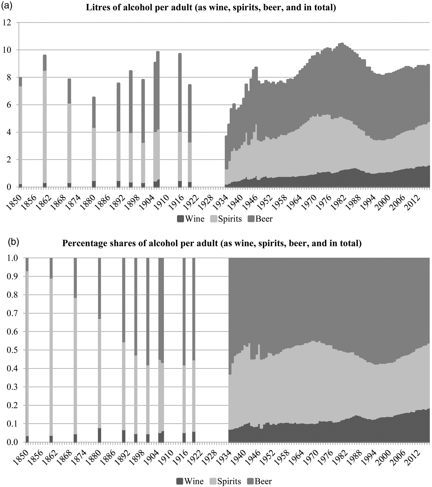
In this section, we describe historical U.S. alcohol consumption, and the differences in alcohol consumption across states. Haughwout and Slater (Reference Haughwout and Slater2018) discuss national, state, and regional trends in U.S. per capita apparent alcohol consumption using annual data, by beverage type, for the 40-year period 1970–2016. They also provide data in incomplete series back to 1850. As these longer-term data show (Figure 1), total U.S. per capita alcohol consumption has risen and fallen significantly over time; but for most years it ranged between 2.0 and 2.5 gallons per capita apart from the period of Prohibition (1920–1933) for which reliable data are not available, and the years immediately following. After Repeal in 1933, total per capita alcohol consumption trended upwards for half a century, to reach a peak at 2.76 gallons of alcohol per capita in 1982. From that peak, per capita consumption of alcohol declined to 2.15 gallons per year for 1993–1998, after which it grew to a new plateau of around 2.33 gallons per year for 2012–2016.
Consumption of Alcohol Per Adult, United States, 1850 to 2016

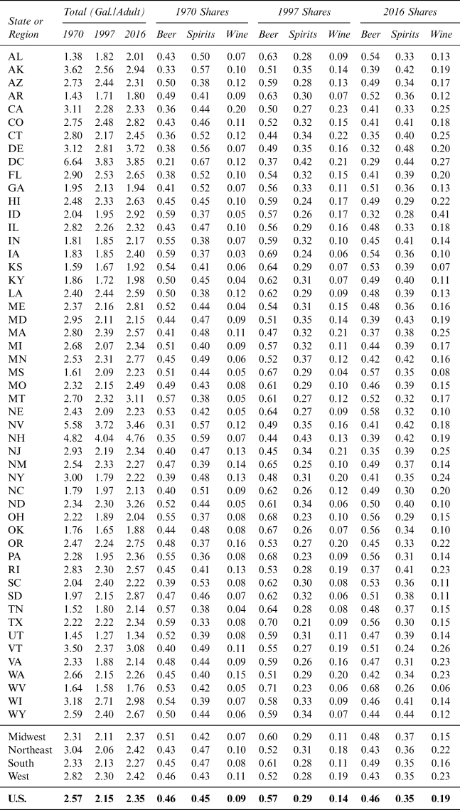
Along with the changes in total consumption, the plots in Figure 1 reveal movements in the mix. Up through the decade of the 1880s, the United States might well have been best described as a whiskey-drinking nation, with spirits accounting for more than half of the total. But ever since then, at least one-half of the nation's alcohol consumption has been in the form of beer. The per capita quantities of beer, wine, and spirits have drifted along with longer-term shifts in total alcohol consumption, and the share of wine has trended upwards slowly, at the expense of both beer and spirits. Still the relative shares of national alcohol consumption have been comparatively stable over five decades, going from (beer, spirits, wine) = (0.463, 0.450, 0.089) in 1970 to (0.459, 0.353, 0.187) in 2016 (Table 1); unlike the world as a whole. As shown by Holmes and Anderson (Reference Holmes and Anderson2017) using data measured on a different basis, U.S. per capita alcohol consumption in the current decade is more than 2.5 times the global average, with larger shares of both beer and spirits and a smaller share of wine. And the U.S. trend is in the opposite direction compared with the global average—with the share of wine rising, and the share of beer falling—such that the United States in this sense is converging towards the rest of the world and somewhat towards more equal shares of the three beverages in the total.
Gallons of Ethanol Consumed per Capita, and Shares of Beer, Spirits, and Wine, for U.S. States, 1970, 1997, and 2016

Notes: Based on population aged above 13 years.
Source: Created by the authors using data from Haughwout and Slater (Reference Haughwout and Slater2018) and NIH/NIAAA (2019).
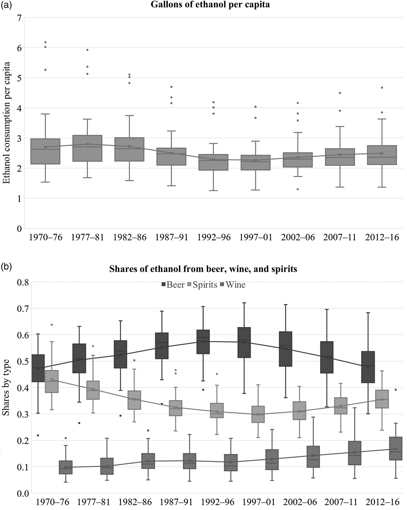
We are also interested in the differences among the 50 states (and the District of Columbia) that contribute to that total, and how those differences have changed. Figure 2 presents box and whiskers plots of state-level data, as five-year averages (seven-year average for 1970–1976), for the shares of total per capita consumption coming from beer, spirits, and wine (Panel a), as well as total per capita consumption (Panel b), for the period 1970–2016; Table 1 summarizes the state-level statistics for the years 1970, 1997, and 2016.Footnote 3 As these comparisons reveal, the national and regional average data mask considerable variation among states. In 2016, total alcohol consumption per person (over age 14) ranged from less than 1.8 gallons in Utah and West Virginia up to well more than 2.8 gallons in 13 states and more than 3.7 gallons in Delaware, the District of Columbia, and New Hampshire (at 4.8 gallons, perhaps reflecting illicit or legal border trade with consumers from higher-taxed neighboring states and Canada). The mix also varies considerably among the states. Beer's share of total alcohol in 2016 ranged from 29% in the District of Columbia to 68% in West Virginia; spirits’ share ranged from 24% in Vermont to 48% in Delaware; and wine's share ranged from 6% in West Virginia to 41% in Idaho. Some states saw radical changes in consumption shares over time, such as Idaho with beer and wine shares of 59% and 5%, respectively, in 1977, and 32% and 41% in 2016—potentially grounds for skepticism about some of the data.
Consumption of Alcohol in U.S. States, Five-Year Averages, 1970 to 2016

III. Convergence among States in Per Capita Alcohol Consumption and the Mix
Against the background of these general trends we now turn to a deeper consideration of the extent to which states are becoming more or less similar in their alcoholic beverage consumption habits. Using various measures, we find that, if anything, consumption patterns have diverged among states since the late 1990s. In subsequent sections we look into potential explanations.
Figure 2 offers informal insight into the extent to which the per capita consumption of alcohol and the shares coming from beer, spirits, and wine vary among states. The plots in Panel a show considerable variation in average per capita consumption of ethanol across the states in each five-year interval, but suggest consumption per capita has converged somewhat across states while generally trending down. Comparing the plots for the 1970s and 1980s to the early 2000s reveals some decrease in the variance of consumption per capita. However, the plots in Panel b reveal more than a simple convergence in consumption patterns. Across the 40-year period, the national average share of beer rose and fell symmetrically; in the latter period, shares of both spirits and wine rose at the expense of beer. These plots also reveal a noticeable increase in the variance of beer and wine shares among states. Although national alcohol shares among types of alcohol are becoming more equal, on average, the states may be diverging in terms of the extent to which they specialize in beer, spirits, or wine.
This question of the nature and extent of convergence can be approached more formally. We use the same three indicators of convergence employed by Holmes and Anderson (Reference Holmes and Anderson2017) applied to U.S. state-level data. First, for each year in the sample, using the state-level data, a coefficient of variation (CV i) was computed for total per capita consumption of ethanol, as well as for per capita consumption of beer, spirits, and wine. Second, a beverage consumption intensity index, CI ij for beverage i in state (or region) j can be computed for any given time period as CI ij = f ij/f i, where f ij is the fraction of total alcohol consumed as beverage i in state (or region) j and f i is corresponding national fraction of total alcohol consumed as beverage i. An estimate of CI in > 1 indicates state j is comparatively specialized in consuming beverage i. Third, using the same measure, f ij, an index, ω jk can be used to measure the similarity of the alcoholic beverage mix of one state, i to that of another state (or the nation as a whole), k and therefore to study changes in similarity of the alcoholic beverage mix among the 50 states and the District of Columbia over time:
 $$\matrix{ {\omega _{\,jk} = \displaystyle{{\mathop \sum \nolimits_{i = 1}^3 f_{ij}f_{ik}} \over {{\left( {\mathop \sum \nolimits_{i = 1}^3 f_{ij}^2} \right)}^{{1 \over 2}}{\left( {\mathop \sum \nolimits_{i = 1}^3 f_{ik}^2} \right)}^{{1 \over 2}}}}\;} \cr} $$
Using Equation (1), for each five-year period of the data,  $\bar{t}$, we computed a 51 × 51 matrix of ω jk,
 ${\rm \Omega} _{\bar{t}}$ representing the 50 states and the District of Columbia, and we added a row (and a column) to include measures of similarity between each of these 51 and the nation as a whole, to make it 52 × 52.Footnote 4 The mean size of the index, ω jk is a useful measure of the degree of similarity among states, whether it is computed for an individual state, k, as a measure of its similarity to all others,
 $\bar{\omega} _k$, or across the entire population of states,
 $\bar{\bar{\omega }}$, to measure the overall similarity among them.Footnote 5
Fogarty and Voon (Reference Fogarty and Voon2018) discuss an issue with the similarity index measure noted by Mills (Reference Mills2018). The adding-up constraint for the alcohol shares implies restrictions on the covariance relationships across beer, wine, and spirits. Mills (Reference Mills2018) details the consequences of this issue and provides a solution: use the trace of the centered log-ratio covariance matrix for alcohol shares: tr(Γt), for period t. This measure, as defined by the matrix in Equation (2), approaches zero as states become more similar in their consumption mix.
 $$\matrix{ {{\rm \Gamma} _t = {\rm cov}\lcub {{\bf F}_{it},{\bf F}_{lt}} \rcub \;} \cr} $$
Here i, l = wine, beer, and spirits; and in period t,  ${\bf F}_{it} = \left[ {\ln \left( {\displaystyle{{f_{it1}} \over {{\bar{f}}_{t1}}}} \right), \ldots, \ln \left( {\displaystyle{{f_{itJ}} \over {{\bar{f}}_{tJ}}}} \right)} \right]$ for state 1, 2, …, J; f itj is the share of good i in state j t; and
 $\bar{f}_{tj}$ is the geometric mean of the alcohol shares in state j.
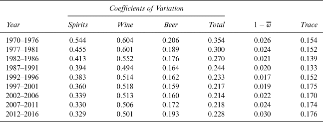
To summarize our findings regarding convergence, three measures of variation in per capita alcohol consumption among U.S. states are reported in Table 2: (1) the coefficients of variation for per capita consumption of spirits, wine, and beer and total alcohol, (2) an overall index of the similarity of the shares of spirits, wine, and beer in the total, and (3) the trace of the centered log-ratio covariance matrix for alcohol shares. The measures are calculated for five-year periods using annual data for the 50 states and the District of Columbia for 1970–2016. For convenience,  $1- \bar{\bar{\omega }} $ is shown for the similarity index instead of
 $\bar{\bar{\omega }}$ such that higher values indicate greater variance. While the patterns in the CV measures are less clear, the similarity index and trace both suggest that consumption patterns across states became more similar from 1970 until the early 1990s, but since then the consumption patterns diverged. These findings update and reinforce those from Fogarty and Voon (Reference Fogarty and Voon2018) but with slightly different timing of the reversal in the trend.
Convergence Measures: Coefficient of Variation, Similarity Index, and Trace

Notes: Based on population aged above 13 years.
Source: Created by the authors using data from Haughwout and Slater (Reference Haughwout and Slater2018).
IV. Accounting for Differences among States in Per Capita Alcohol Consumption
As noted, while representative consumers in most U.S. states drink more beer than any other form of alcohol, they vary in terms of how much they drink and the extent to which they are specialized in beer drinking; and these differences are persistent, though not totally unchanging.Footnote 6 What can account for these persistent differences among states? Candidate explanations include interstate differences in prices and income among consumers, differences in policies, and differences in tastes—some of which might be connected to the causes of the differences in policies and prices.
In the context of international data, both Colen and Swinnen (Reference Colen and Swinnen2016) and Holmes and Anderson (Reference Holmes and Anderson2017) focus on per capita income as a primary consideration (finding some evidence of an inverted U-shaped relationship between per capita income and alcohol consumption) along with prices paid by consumers (and taxes as an influence on them), as factors influencing per capita demands among nations. In our context, with U.S. states playing the role of nations, state-level data are available on measures of per capita income, but we do not have access to good time-series data on state-level prices.Footnote 7 These conventional variables belong in any economic model of consumer behavior, but prices and income alone are unlikely to account for the large and persistent differences in alcohol consumption that we observe among U.S. states.
A more obvious answer for a non-economist might be cultural differences—we eat and drink in ways that our grandparents, parents, friends, and neighbors did because that is what they taught us to do; some tastes are acquired, some habits are persistent if not addictive, and we identify to some extent with the culture from which we came. If these aspects are important, in general and on average we would expect to observe Americans of, say, German descent drinking significantly more beer and less wine per capita, compared with other Americans of, say, Italian descent, holding other factors constant. Data are available on this aspect of the demographic structure of the population of U.S. states which, within any particular state, might not change quickly enough to account for changes over time, but is significantly different among states in ways that could account for persistent spatial differences.
The United States is a physically and economically large and diverse geopolitical entity. Space matters. Most U.S. wine is produced within 100 miles of the Pacific Ocean, mainly in California. Most Americans live far from there. In the United States wine tends to be consumed at higher rates per capita in the states where it is produced, in the same way that wine tends to be consumed at higher rates per capita in countries that are major wine producers and exporters. Differences in comparative advantage and historical patterns of production among nations have contributed to cultural norms and traditions related to alcohol consumption that have carried forward with those who emigrated to the United States.
Among the 50 states and Washington, DC, populations differ ethnically and culturally in ways that are likely to matter for alcohol consumption. Much of the country—especially in the Midwest—was settled by Northern Europeans who are traditionally drinkers of beer or spirits, rather than wine; Southern Europeans, who are traditionally more likely to be wine drinkers, are more predominant in the Northeast. Other significant ethnic groups—Hispanics, African-Americans, and Asians—are also traditionally more likely to be beer drinkers than wine drinkers.
Combining U.S. data on ancestry (measured as the proportions of the population coming from different national ethic origins) with data on the internationally diverse shares of national alcohol consumption coming from beer, spirits, and wine, allows us to measure the degree to which states (or counties or other geographical areas) have historical cultural ties to beer, spirits, and wine drinking nations. Specifically, we measure the “ancestral” (predicted) rate of consumption of alcohol type i in geographical area, j, A ij as a weighted average of the rate of consumption of that alcohol type across nations (v ik for type i in country k during 1961–1964 from Holmes and Anderson, Reference Holmes and Anderson2017) where the weights are the proportions of residents in area j having ancestry from country k, p jk:
 $$\matrix{ {{A}_{{ij}} = \mathop \sum \limits_{{k} = 1}^{K} {v}_{{ik}}{p}_{{jk}}} \cr} $$
For example, suppose 60% of the residents of County X identify their primary ancestry as French and 40% as German. Since French beer consumption was 0.48 gallons (of ethanol) per capita, and German beer consumption was 1.46 gallons (of ethanol) per capita, the ancestral rate of consumption of beer for County X is 0.87 (= 0.6 × 0.48 + 0.4 × 1.46) gallons (of ethanol) per capita. The ancestral rate of beer consumption, for example, varies greatly across the United States. Owing primarily to the large Hispanic shares of the population, the Southwest region of the country has high ancestral beer consumption. Conversely, states in the Northeast typically have lower ancestral beer consumption owing to large Southern European population shares. Maps in the SOM illustrate how this measure varies across states.
In addition to ethnicity, culture and religion play a role in current consumption patterns. In some states, large proportions of the population belong to religions that preach temperance or complete abstinence from consuming alcohol. Partly for those reasons, policies affecting the marketing and consumption of alcohol vary systematically among the states as a legacy of Prohibition and its Repeal. When Prohibition was repealed, it was on the condition that individual states could define their own laws governing the production and sale of alcohol, an outcome that would leave as its legacy a byzantine and bizarre set of policies that continue to hamstring alcoholic beverage producers and marketers today. The policies have changed over time in ways that complicate the analysis of markets. Several other socioeconomic variables may be correlated with beer and wine consumption, such as obesity prevalence, per capita income, educational attainment, and political orientation (e.g., as revealed in results from the 2016 U.S. Presidential election).Footnote 8 The SOM provides a brief discussion of our measures of these variables.
V. Demographic Influences on Demand for Alcohol: State-Level Analysis
We estimated econometric models to examine demographic influences on demand using annual state-level data on adult per capita ethanol consumption by main type of alcohol (beer, wine, spirits) for 1970–2016 taken from Haughwout and Slater (Reference Haughwout and Slater2018) and data on prices from the Bureau of Labor Statistics.Footnote 9 These prices are available only for four aggregated U.S. regions, and for the aggregated product categories of malt beverages, vodka, and wine. To derive state-specific prices, we adjusted the regional prices using state beverage-specific tax rates accessed online from the Alcohol and Tobacco Tax and Trade Bureau as well as the Tax Foundation (U.S. Treasury/TTB, 2005; U.S. Treasury/TTB, 2013; U.S. Treasury/TTB, 1984–2015; Tax Foundation, 2013). The results in this section reveal some shortcomings of using these data to estimate elasticities and identify relationships between policy, socioeconomic patterns, and alcohol demand.
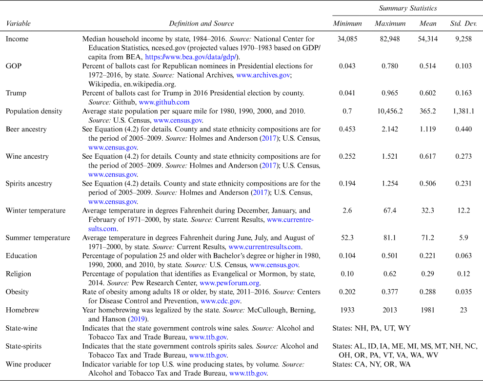
The models include various measures of socioeconomic variables. State-level data on measures of ethnicity and household income come from the U.S. Census (U.S. Census Bureau American FactFinder, 2018). The data on ethnicity are combined with international data on country-specific consumption shares by alcohol type from Holmes and Anderson (Reference Holmes and Anderson2017) to derive an ancestral beverage consumption measure using Equation (3). The models also include measures of national election results, average winter and summer temperatures, the share of population with a bachelor's degree, the share of population that belongs to a religion that abstains from alcohol, the obese share of the adult population, the year when homebrewing was legalized, and an indicator of wine production volume. Table 3 provides a summary of the explanatory variables used and the data sources.
Variable Definitions, Summary Statistics, and Data Sources

The models we estimate in this section (using state-level data) and the next section (using regional scanner data) can be thought of as belonging to the class of “differential demand systems” models, perhaps best exemplified by the Rotterdam model (Theil, Reference Theil1965). When we take a logarithmic differential approximation to a general model of demand as a function of prices and total expenditure, which is the first step in deriving models of this class, the resulting equation is linear in proportional (logarithmic differential) changes in the arguments, each multiplied by its corresponding elasticity. A more practical discrete-time variant includes variables in logarithmic differences rather than logarithmic differentials, and is indistinguishable from a first-differenced version of a constant elasticity (i.e., “double-log”) model, though it is derived from a different conception. With some further manipulation (as in the derivation of the Rotterdam model, applied later in this article) the variables and associated coefficients can be transformed into forms that allow Slutsky symmetry and other restrictions to be imposed in a system of demand equations (e.g., Okrent and Alston, Reference Okrent and Alston2011).
Models like this are typically applied to time-series data, such that the logarithmic differentials are growth rates of variables. Here we focus on differences among states associated with demographic variables (which are comparatively constant over time within states but vary among states) rather than differences within states over time associated with prices, which calls for a variation in the approach. Specifically, instead of modeling year-to-year differences within a state, we model differences relative to the mean for all states, within a year, which is helpful for measuring the effects of socioeconomic and demographic characteristics of populations, including income; less so for measuring the effects of prices.
A. Single-Equation Models of Demand for Beer, Wine, and Spirits
In the first application using state-level data, we leave the model in the simple form in which the coefficients can be interpreted directly as elasticities, and we estimate demand equations without imposing any cross-equation restrictions or other restrictions from economic theory apart from homogeneity of degree zero in prices and income (or total expenditure on the relevant group of goods). We estimate single-equation models of per capita demand for each of the three types of alcohol, in which the demand equation for beverage i in state k in year t is defined as:
 $$\matrix{ {{\rm D}q_{ikt} = \eta _{iI}{\rm D}y_{kt} + \mathop \sum \limits_{\,j = 1}^J \eta _{ij}{\rm D}p_{\,jkt} + {\bf \delta} _i{\rm D}{\bf a}_{ikt} + \epsilon _{ikt}} \cr} $$
In this and subsequent equations, the operator D denotes that each variable is expressed as a logarithmic difference relative to the mean of that variable across all states during year t. The per capita quantity of good i in state k in year t is q ikt, and  ${\rm D}q_{ikt} = \log q_{ikt}-\log \bar{q}_{it}$; y kt is per capita income in state k in year t, and
 ${\rm D}y_{kt} = \log y_{kt}-\log \bar{y}_t$; similarly, p jkt is the price of good j in year t for state k and
 ${\rm D}p_{jkt} = \log p_{jkt}-\log \bar{p}_{jt}.$ The price coefficient η ij, is the uncompensated (or Marshallian) elasticity of demand for good i with respect to the price of good j; the coefficient η iI is the elasticity of demand for good i with respect to per capita income. Both the beverage prices and per capita income were deflated by the consumer price index for all goods (CPI), representing the prices of all other goods, such that the demands are restricted to be homogeneous of degree zero with respect to prices of alcoholic beverages and all other goods (the CPI) and per capita income. A vector of demand shift variables is represented by
 ${\bf a}_{it}$, where
 ${\rm D}{\bf a}_{ikt} = \log {\bf a}_{ikt}-\log {\bar{\bf a}}_{ikt}$; the vector of coefficients,
 ${\bf \delta} _{\rm i}$, can be interpreted as elasticities of demand for good i with respect to the respective elements of the vector of demand shift variables (unless the variables are 0–1 indicator variables). Descriptions of the variables can be found in Table 3. Not listed in the table are “NH,” “DE,” “DC,” and “NV,” which are state fixed effects included for states with exceptionally high alcohol sales owing to border trade or tourism.
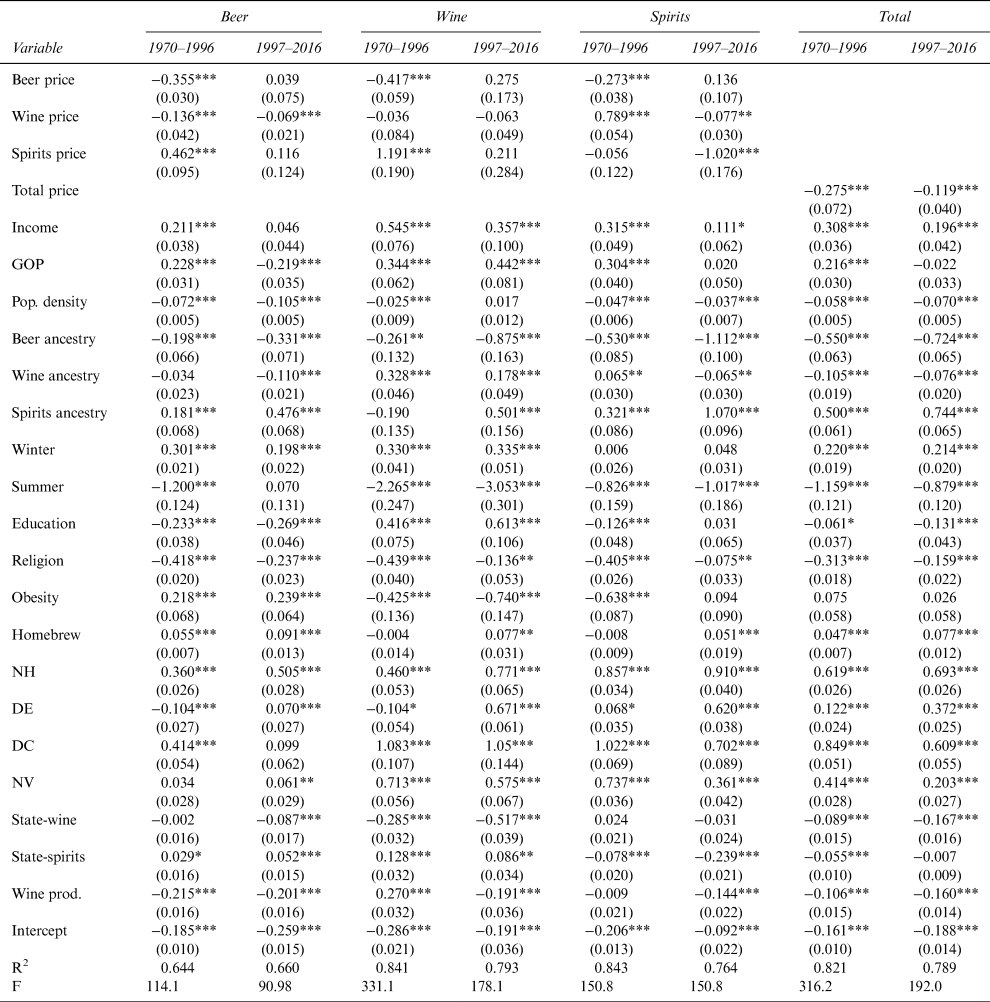
As discussed earlier and as shown in Figure 2 (see also figures in the SOM), the trends in alcohol consumption were quite different in the last 20 years of the 47-year history, 1970–2016. Considering those differences, and after some limited pretesting, we opted to split the data and estimate the model separately for the two periods, 1970–1996 and 1997–2016. A simple Chow test applied to Equation (4) rejects the null hypothesis that there is no structural break. For each sub-period we estimate per capita demand equations separately for beer, wine, and spirits. The results are summarized in the first six columns of Table 4. Each of the models appears to fit the data reasonably well, with a high proportion of statistically significant effects. The model for beer (in the first two columns) does generally less well than the others in terms of both overall fit and consistency of estimated effects with expectations.
Estimates of Single-Equation Models of Demand Using State-Level Data, 1970–2016

Notes: Chow test for structural break at 1997: F = 1.9047, p-value = 0.007816. N = 1,377 for 1970–96; N = 1,020 for 1997–16. First-stage estimation.
Sources: Created by the authors using consumption data from Haughwout and Slater (Reference Haughwout and Slater2018), prices from the Bureau of Labor Statistics and Alcohol and Tobacco Tax and Trade Bureau, and other sources as described in Table 4.
The first four rows of Table 4 report the estimates of the uncompensated price elasticities of demand. It is encouraging that the point estimates of the own-price elasticities are all negative (except for that of beer in the earlier period, 1970–1996), but the estimated elasticities are generally smaller in magnitude than would be expected, and many of them are not statistically significantly different from zero. These outcomes probably reflect the limitations of the price data, which are crude estimates derived from regional prices of proxy beverages combined with state-specific tax rates, and do not account for the within-category variation in the mix of types of beer, wine, and spirits consumed across states and over time. Errors in the variables would cause the elasticity estimates to be attenuated towards zero, and we can surmise that more detailed and more precise price data are necessary to extract more meaningful estimates of price elasticities.
However, in the present context, we are more interested in the effects of the demographic variables included in the model, including per capita income. In brief, on these aspects the results are mixed. Many of the effects are in directions we would have expected—for example, per capita consumption of all three types of alcohol decreases with increases in the share of population belonging to a religion that abstains from alcohol; or with an increase in population density (rural residents tend to drink more)—but in some cases we see switches in signs of effects between sub-samples, and some results are surprising. The set of coefficients for the alcohol ancestry variables are among the most interesting. They support the view that heritage plays a role in alcohol consumption. However, the results for beer ancestry are surprising. An increase in our index of ancestral beer consumption is associated with lower rates of per capita consumption of all forms of alcohol, including beer; in each sub-period the elasticity is smaller in magnitude for beer than for wine and spirits, but these elasticities are all highly statistically significant. In keeping with expectations, an increase in ancestral wine consumption is associated with higher rates of per capita consumption of wine and lower rates of per capita consumption of beer and spirits. An increase in ancestral spirits consumption is associated with higher rates of per capita consumption of beer and wine (in the later period), as well as spirits. In subsequent sections we explore how these findings may change as we impose cross-equation restrictions, in a complete system of demand equations for alcoholic beverages, and when we use data for less-aggregated categories of alcoholic beverages and at finer spatial aggregation.
B. A System of Demand for Beer, Wine, and Spirits: Structure of the Model
We use a demand systems approach to estimate state-level per capita demands for beer, wine, and spirits, which allows us to impose cross-equation restrictions implied by economic theory. As noted, the single-equation models estimated earlier bear some similarity to equations of the Rotterdam model.Footnote 10 Here, we specify a Rotterdam model of demand to estimate the effects of demographic variables on demand for different categories of beer and wine, controlling for the effects of relative prices and total expenditure on the beverages included in the model—that is, treating the alcoholic beverages included in the model as a weakly separable group. This is a differential demand system model that has often been used to estimate models of demand for alcoholic beverages including beer, wine, and spirits (e.g., Clements and Selvanathan, Reference Clements and Selvanathan1988; Clements and Selvanathan, Reference Clements and Selvanathan1991; Selvanathan, Reference Selvanathan1991; Selvanathan and Selvanathan, Reference Selvanathan and Selvanathan2005).
In order to estimate elasticities that are conditional on total per capita expenditure on all goods and not just expenditure on alcohol, we implement a two-stage approach, as discussed by Edgerton (Reference Edgerton1997). For the first stage, we use estimates of a single-equation model, as in Equation (4), of per capita demand for total alcohol with the variables in logarithmic differential form, as represented in Equation (5):
 $$\matrix{ {{\rm D}Q_{kt} = \eta _G^M {\rm D}y_{kt} + \eta _{GP}^M {\rm D}P_{kt} + \delta {\rm D}{\bf a}_{{\rm kt}}\; + \epsilon _{kt}} \cr} $$
Here,  ${\rm D}Q_{kt} = \mathop \sum \limits_{{\rm i} = 1}^{\rm I} \bar{s}_{ikt}{\rm D}q_{ikt}$ is the Divisia total volume index of alcohol consumption in state k in period t, where, for state k in period t,
 $\bar{s}_{ikt}$ represents the arithmetic mean of (a) the budget share of good i in that state and (b) the budget share of good i on average across all of the states; P kt is a price index of alcoholic beverages; and y kt is a per capita expenditure on all goods (or income). Both the beverage prices and per capita income were deflated by the consumer price index for all goods (CPI), representing the prices of all other goods.
In Equation (5)  $\eta _G^M $ is the elasticity of total per capita demand for alcohol (in quantities as indicated by the volume index for the group) with respect to expenditure on all goods (or income),
 $\eta _{GP}^M $ is the Marshallian elasticity of demand for alcohol (the group) with respect to the group price, conditional on per capita expenditure on all goods (or income), and the vector of coefficients,
 ${\bf \delta} $, can be interpreted as elasticities of demand for alcohol with respect to the corresponding elements of the same vector of demand shift variables that were included in the single-equation models of demand for beer, wine, and spirits. Estimates of these elasticities are reported in the last two columns of Table 4, where they can be compared with the counterpart estimates for the individual categories of beer, wine, and spirits; they are discussed later, in conjunction with those for the second stage allocations of alcohol expenditure among those categories.
In the absolute price version of the base Rotterdam model, used to represent the second-stage allocations, the demand equation for good i in time t is defined as shown in Equation (6).
 $$\matrix{ {{{\bar{ s}}}_{{ ikt}}{\rm D}{ q}_{{ ikt}} = { \beta} _{ i}{\rm D}{ Q}_{{ kt}} + \mathop \sum \limits_{{ j} = 1}^{ J} { \alpha} _{{ ij}}{\rm D}{ p}_{{ jkt}}{ \;} + { \epsilon} _{{ ikt}}} \cr} $$
The Slutsky coefficient for goods (i, j) is α ij, and these coefficients satisfy the homogeneity restriction,  $\mathop \sum \limits_{j = 1}^J \alpha _{ij} = 0{\rm \;} $ and the symmetry restriction, α ij = α ji. The elasticity of demand for good i with respect to group expenditure can be computed as
 $\eta _i^E = \beta _i/s_i$, the Hicksian (compensated) elasticity of demand for good i with respect to the price of good j is calculated as
 $\eta _{ij}^H = \alpha _{ij}/s_i$, and the Marshallian (uncompensated) elasticity of demand for good i with respect to the price of good j conditional on group expenditure is calculated as
 $\eta _{ij}^E = \lpar {\alpha_{ij}-\beta_is_j} \rpar /s_i$. Expanding the model to include a vector of N demographic demand shifters,
 ${\bf a}_{kt} = \lsqb {a_{kt1}, \ldots, a_{ktN}} \rsqb $ with corresponding coefficients
 ${\bf \delta} _i = \lsqb {\delta_{i1}, \ldots, \delta_{iN}} \rsqb $ in the equation for beverage type i, yields Equation (7):
 $$\matrix{ {{{\bar{ s}}}_{{ ikt}}{\rm D}{ q}_{{ ikt}} = { \beta} _{ i}{\rm D}{ Q}_{{ kt}} + \mathop \sum \limits_{{ j} = 1}^{ J} { \alpha} _{{ ij}}{\rm D}{ p}_{{ jkt}}{ \;} + {\bf \delta} _{ i}{\rm D}{\bf a}_{{ kt}} + { \epsilon} _{{ ikt}},} \cr} $$
where  $\mathop \sum \limits_{{j} = 1}^{ J} \delta _{jn} = 0\; {\rm for}\; n = 1, \ldots, N.$Footnote 11
As discussed by LaFrance (Reference LaFrance1991) an endogeneity issue arises when modeling demand for a weakly separable group of goods because, by construction, group expenditure cannot be exogenous when it is computed as the sum of the prices times quantities demanded for the goods included in the group. To circumvent this endogeneity issue, we replace the Divisia volume index, DQ kt in Equation (7) with the fitted values from Equation (5),  $\widehat{{{\rm D}Q}}_{kt}$—effectively using per capita income as an instrument for group expenditure:
 $$\matrix{ {{\bar{s}}_{ikt}{\rm D}q_{ikt} = \beta _i{\widehat{{{\rm D}Q}}}_{kt} + \mathop \sum \limits_{\,j = 1}^J \alpha _{ij}{\rm D}p_{\,jkt}{\rm \;} + {\bf \delta} _i{\rm D}{\bf a}_{kt} + \epsilon _{ikt}} \cr} $$
In other words, the Rotterdam model is estimated using two-stage least squares for which the first stage is represented by Equation (5) and the second stage is represented by Equation (8). Estimating the model in this fashion allows us also to approximate elasticities conditional on total expenditure on all goods (denoted by superscript M), as discussed by Carpentier and Guyomard (Reference Carpentier and Guyomard2001) and Okrent and Alston (Reference Okrent and Alston2011), as well as elasticities conditional on group expenditure (denoted by superscript E), using just the second-stage estimates. The various expenditure and price elasticities conditional on total expenditure, respectively, are calculated as:
 $$\matrix{ {\eta _i^M = \eta _i^E \eta _G^M} \cr} $$
 $$\matrix{ {\eta _{ij}^M = \eta _{ij}^E + s_j^E \eta _i^E \eta _i^E \left( {\displaystyle{1 \over {\eta_j^E}} + \eta_{GP}^M} \right) + s_j^E s_G^M \eta _G^M \eta _i^E \lpar {\eta_j^E -1} \rpar } \cr} $$
•
 $\eta _i^M = $ the elasticity of demand good i with respect to total expenditure on all goods (the income elasticity of demand for alcohol of type i),
•
$\eta _i^E = $ the elasticity of demand for good i with respect to group expenditure,•
$\eta _G^M = $ the elasticity of expenditure on the group with respect to total expenditure (i.e., the income elasticity of demand for the group of alcoholic beverages being modelled),•
$\eta _{ij}^M = $ the Marshallian elasticity of demand for good i with respect to price j conditional on total expenditure on all goods,•
$\eta _{ij}^E = $ the Marshallian elasticity of demand for good i with respect to price j conditional on group expenditure,•
$\eta _{GP}^M = $ the Marshallian elasticity of demand for the group with respect to the group price conditional on total expenditure on all goods (i.e., income),•
$s_j^E = $ the within-group budget share for good j—total expenditure on the good as a share of total expenditure on the group, and•
$s_G^M = $ the budget share for the group—total expenditure on the group as a share of total expenditure on all goods.


C. A System of Demand for Beer, Wine, and Spirits: Estimation Results
As noted in the discussion prior to estimation of the single-equation models of demand, in our dataset the several demographic variables are measured at infrequent intervals (every ten years) relative to the consumption data (annual observations), and the measures do not change quickly over time when they are measured. Hence it is not possible or sensible to employ the model, as in Equations (5) and (8), first differencing temporally ordered data, seeking to estimate the influence of the demographic variables on demand. Alternatively, and like the single-equation models of demand, the Rotterdam model can be applied to data differenced relative to the mean across all the observations (or some other baseline) in the same period, exploiting the variation in the cross-section where temporal variation is insufficient. In our application, instead of differencing the variables across time, they are differenced relative to the mean across all of the states in the same time period.Footnote 12 Also, as discussed in relation to the single-equation models and for the same reasons, we opted to split the data and estimate the model separately for the two periods, 1970–1996 and 1997–2016.
The results from the first-stage estimation (i.e., Equation (5)) are summarized in the last two columns of Table 4, representing the model for total alcohol demand per capita in the two time periods, 1970–1996 and 1997–2016.Footnote 13 The estimated income elasticity of demand for alcohol is in the range for a “necessity” good:  $\eta _G^M = \; $ 0.308 in 1970–96 (0.196 in 1997–16), and the estimated own-price elasticity of demand, conditional on total income (expenditure on all goods) is in the inelastic range:
 $\eta _{GP}^M = -$ 0.275 in 1970–96 (
 $\eta _{GP}^M = -$ 0.119 in 1997–16). That is, a 1% increase in per capita income results in a 0.308 (0.196)% increase in per capita expenditure on alcohol, and a 1% increase in the composite price of alcohol results in a 0.275 (0.119)% decrease in the total quantity of alcohol demanded.
The other reported estimates can be interpreted as elasticities as well. Many of the elasticities are statistically significantly different from zero, and reasonably consistent in size as well as in the sign of the effect across the two time periods, 1970–96 and 1997–2016. Specifically, predicted per capita demand for alcohol is consistently estimated to be greater in states that had (a) lower population density, (b) lower rates of ancestral consumption of either beer or wine, or higher rates of ancestral spirits consumption, (c) warmer winters, or cooler summers, (d) fewer residents ascribing to a religion that preaches abstaining from alcohol, (e) more liberal attitudes to alcohol as indicated by legalized homebrewing or the absence of state control over wine sales, and (f) less production of wine. Obesity rates did not statistically significantly account for changes in per capita demand for alcohol in either time period. Across the two time periods, the sign or significance of the estimated effect was mixed for other variables such as the proportion of GOP voters or states having state-controlled spirits sales.
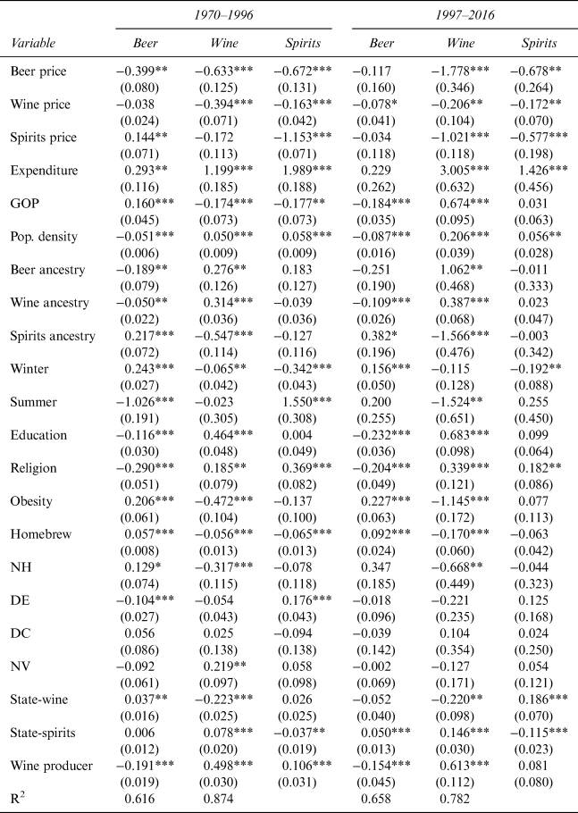
Next, we estimate the second stage of the model, as in Equation (8), representing the allocation of alcohol expenditure among beer, wine, and spirits.Footnote 14 The implied elasticities at the mean of the sample data, conditional on expenditure on alcohol, are reported in Table 5.Footnote 15 The first three columns correspond to the per capita demands for beer, wine, and spirits for the period 1970–1996, and the last three columns for 1997–2016. The first three rows refer to Marshallian (uncompensated) own- and cross-price elasticities of demand, conditional on total expenditure on alcohol. It is encouraging that the point estimates of the own-price elasticities are all negative and measured relatively precisely, but in quite a few cases the cross-price elasticities are—contrary to expectations—also negative, even larger magnitudes, and statistically significant.
Elasticities of Demand for Alcohol from the Rotterdam Model Estimated Using State-Level Data, 1970–2016

Notes: Marshallian price elasticities and expenditure elasticities, conditional total beer and wine expenditure. Second-stage estimation.
Sources: Created by the authors using consumption data from Haughwout and Slater (Reference Haughwout and Slater2018), prices from the Bureau of Labor Statistics and Alcohol and Tobacco Tax and Trade Bureau, and other sources as described in Table 3.
These patterns reflect the fact that the computed elasticities are dominated by “income” effects, with comparatively small compensated price effects. In turn these outcomes probably reflect the issues with the price data, discussed in the context of the single-equation models, such that we cannot place great confidence in the resulting estimates of demand response to price—while hoping, nevertheless, that including these measures may “control” for price effects sufficiently to permit other effects to be measured well. Recall, as discussed in relation to the single-equation models, in the present context, we are particularly interested in the effects of the demographic variables included in the model (described in Table 3), especially the ancestral alcohol consumption variables.
Again, the interpretation of these elasticities is straightforward, but we will highlight a few key results, noting that in this demand systems context, across the three types of alcohol, the sum of the coefficients for each demographic variable equals zero by construction—that is, holding the total expenditure on alcohol constant, any factor that causes an increase in per capita demand for (and, thus, expenditure on) one type of alcohol must cause an offsetting decrease in expenditure on (and, thus, demand for) some other type(s) of alcohol. Many of the effects are in directions we would have expected, but as in the single-equation models reported in Table 4, in some cases we see switches in signs of effects between sub-samples—especially in the case of beer—and some results are surprising.
The estimated “income” effects are plausible: within the group of alcoholic beverages, wine and spirits are “luxuries” while beer is a “necessity” good. In other words, as total per capita consumption of alcohol increases, demand for beer increases slightly, its expenditure share shrinks, and the share of alcohol expenditure increases more substantially for both wine and spirits. This is in a context in which beer commands a relatively large share of total expenditure on alcohol. Many of the other estimated elasticities are also plausible in terms of their signs and sizes, and consistent across the two time periods. For example, decreases in obesity rates, and increases in population densities, rates of participation in abstemious religions, production of wine, and educational attainment, are all associated with decreases in demand for beer, increases in demand for wine, and increases or statistically insignificant effects on demand for spirits. However, several of the other variables had effects that were unstable over time or had unexpected signs, or both. The estimated coefficients on the “GOP” variable suggest that, during the early period 1970–1996, per capita demand for beer increased while demand for both wine and spirits decreased with increases in the proportion of voters supporting Republican candidates in Presidential elections; however, these signs were all reversed during the more recent period, 1997–2016. This is hard to rationalize simply and might suggest a more general problem with the model or the particular measure of political orientation.
Also, as for the single-equation models, the results for ancestral alcohol consumption are surprising and somewhat disappointing. For example, in the estimates for 1970–1997, an increase in beer-drinking ancestry is associated with reduced demand for beer and increased demand for wine and spirits, while an increase in spirits-drinking ancestry is associated with reduced demand for spirits, but increased demand for beer and wine—in both cases exactly the opposite of what was anticipated. These effects are different in the later period, 1997–2016, but still unexpected. The effects of wine ancestry are more consistent with expectations and more consistent over time but, on the whole, the results are at odds with our hypothesis of a direct connection between ancestral and U.S. consumption mixes.
A candidate explanation for these disappointing results using state-level data is aggregation bias. First, rural and urban areas consume differing mixes and quantities of beer, spirits, and wine. Namely, rural areas typically consume more alcohol, as illustrated by the estimates in Tables 4 and 5 of elasticities associated with population densities. Some states include both large metropolitan areas and sparsely populated rural areas, for which many demographic characteristics will differ, along with their alcohol consumption patterns. Some of our data for the state-level analysis were derived by aggregating across counties, but our per capita model is nonlinear. Second, the categories of beer, wine, and spirits are broad. We know that the composition of those categories has varied across places (i.e., between rural and urban and among states) and over time (i.e., with the rise of premium varietal table wine and craft beer that are more important in some contexts than others) in ways that can matter for our analysis, but which we cannot observe using aggregative data. Third, we do not observe prices even for these aggregative categories and are obliged instead to use crude proxies based on regional prices for indicative examples of each type of beverage, and state-specific tax rates. The next section aims to provide more realistic estimates using data disaggregated spatially, temporally, and across product spaces.
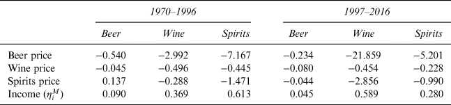
To complete the analysis of this section, elasticities of demand for each type of alcohol with respect to total expenditure on all goods and with respect to prices conditional on total expenditure, calculated according to Equations (9) and (10) and, thus, combining the first-stage estimates from Table 4 and the second-stage estimates from Table 5, are reported in Table 6. Owing to the high level of aggregation across diverse types of beer, wine, and spirits, the poor quality of the price data, and lack of price variation among states, these estimates are to be taken with a grain of salt. Some of the elasticities are plausible, but several are not.
Elasticities of Demand from the Rotterdam Model, Conditional on Total Expenditure on All Goods, U.S. States

Notes: Marshallian price elasticities and expenditure elasticities, conditional on income. Calculated from first- and second-stage estimates as described in Equations (9) and (10).
Sources: Created by the authors using consumption data from Haughwout and Slater (Reference Haughwout and Slater2018), prices from the Bureau of Labor Statistics and Alcohol and Tobacco Tax and Trade Bureau, and other sources as described in Table 3.
VI. Demographic Aspects of Demand for Beer and Wine: Evidence from Scanner Data
The analysis of the previous section used relatively aggregated data at the level of states, in long annual time series. Those data have the disadvantage that the prices are measured poorly, and do not vary much over space, while the per capita demographic variables do not vary much over time, within a state. Now we turn to an analysis using data with a higher degree of cross-sectional variation and better measures of prices. Aggregation is also an issue for the categorization of beer and wine; the product segments within each category (beer and wine) have distinct trends. Namely, the decline of U.S. beer consumption and increase in wine consumption over the past 20 years has coincided with a trend to premiumization in the markets for both beer and wine. Our goal in this section is to further dissect these spatial and temporal alcohol consumption patterns within the United States, and to do this we disaggregate states into designated market areas (DMAs) and disaggregate both beer and wine into sub-categories. The results are much more satisfactory and more consistent with expectations than those from the analysis using the more aggregative state-level data, supporting our conjecture that those estimates might suffer from aggregation bias.
An initial motivation for this work was to understand the recent surge in demand for craft beer. What is craft beer though? The Brewers Association (2018) defines a craft brewery as one producing six million barrels of beer or less annually, not being 25% or more owned by a non-craft alcohol industry member, and brewing the majority of its total beverage alcohol volume from traditional or innovative brewing ingredients (flavored malt beverages are not included). The craft and macro segments of the beer industry have become quite distinct and segmented, with diverging market trajectories. Specifically, the craft segment has realized consistent growth during the 21st century whereas large breweries have seen a continuing decline in sales. In 2016, U.S. craft beer sales rose by 10% to $23.5 billion, accounting for 12.3% of United States beer sales volume and 21.8% of sales value. From 2008 to 2016, the number of craft breweries increased from 1,574 to 5,234 (Brewers Association, 2018). We conjecture that in places where craft beer is relatively popular, compared with macro beer, wine consumption per capita might also be relatively high, reflecting the types of socioeconomic and demographic influences that were revealed in our examination of state-level consumption trends and demographics.
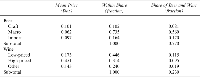
Scanner sales data from Nielsen are used in the estimations.Footnote 16 The data include close to two billion observations of store-level, UPC specific, weekly sales totals covering thousands of brands of beer and wine for 270 metropolitan areas, or DMAs. The composition of the dataset by store-type is 76% grocery, 14% drug, 4% mass merchandiser, 4% convenience, and 2% liquor stores. Owing to differences across states in laws governing the sale of alcohol in stores, only grocery store sales are used. The data are aggregated to DMA-specific monthly totals for three categories of beer (craft, macro, and imported) as well as three categories of wine (low-priced dry, high-priced dry, and other, where “dry” includes sparkling wine as well as still wine, and “other” includes sweet wine and fortified wine). The resulting data set for beer is an unbalanced panel consisting of 19,790 observations, across 181 DMAs, and 120 time periods. For wine, the data set includes 19,985 observations, across 182 DMAs, and 120 time periods. Table 7 provides mean prices and expenditure shares of each beer and wine category; shares are reported as within-category means.Footnote 17
Prices and Expenditure Shares of Beer and Wine Categories, 2006–2015

Notes: Shares calculated at the mean of all DMAs across all months.
Source: Created by the authors using data from Nielsen.
County-level ethnicity and household income data come from the U.S. Census. These are aggregated to the DMA level and then merged with Nielsen scanner data. International data on country-specific consumption shares by alcohol type are borrowed from Holmes and Anderson (Reference Holmes and Anderson2017). By merging the census ethnicity data with national consumption volumes, an ancestral beverage consumption measure is created. Ancestral consumption of beverage k for a particular region (here DMA j), A jk is defined in Equation (3) as the sum of the share of that region's population from each country i, multiplied by the per capita consumption of beverage k in that country (using county-level ancestry data from the United States Census Bureau American FactFinder for the period 2005–2009).
We apply the same two-stage approach described in the previous section to estimate the effects of ancestry and other demographic variables on demand for different categories of beer and wine, controlling for the effects of relative prices and total expenditure on the beverages included in the model, using differential demand systems models. As with the state-level data, the demographic variables are measured at infrequent intervals (annual observations) relative to the consumption data (monthly observations), and the measures do not change quickly over time when they are measured. Hence, in our application, instead of differencing the variables across time, they are differenced relative to the mean of all DMAs in the same time period.Footnote 18
We first estimate single-equation logarithmic differential models of demand for total beer, total wine, and total beer and wine as a function of the own price and income (i.e., expenditure on all goods) deflated by the CPI for all goods, as in Equation (5). Then we estimate systems of equations, specified using the Rotterdam model, to model the allocation of expenditure on both beer and wine across three categories of beer (craft, macro, and import) and three categories of wine (low-priced dry, high-priced dry, and other), as in Equation (8)—using the predicted values of the Divisia volume index from the first-stage estimates rather than the directly computed values. Only DMAs with both wine and beer sales in grocery stores are included in the estimation.
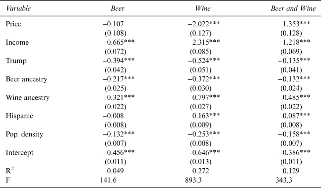
Results from the single-equation models of demand for beer and wine are reported in Table 8.Footnote 19 The models for beer and wine perform reasonably well; less so the model for beer and wine combined. The reported coefficients represent elasticities of demand, and the estimates are precise, generally plausible, and consistent with expectations. The first column represents the demand for beer. The own-price elasticity of demand (conditional on total income) and income elasticity of demand for beer are inelastic (–0.107, 0.665). In the second column, the own-price elasticity and income elasticity of demand for wine are highly elastic (–2.022, 2.315). Combining beer and wine together, in the third column of Table 8 the own-price elasticity of demand is positive (1.353), raising some doubts about whether this aggregation is appropriate, and the income elasticity is elastic (1.218). Turning to the demographic variables, consumers in DMAs with a higher proportion of voters supporting Republican candidates in Presidential elections demand less beer (–0.394) and less wine on average (–0.524), as well as less total beer and wine on average (–0.135); the same is true for consumers in more urban DMAs—that is, with higher population density (–0.132, –0.253, –0.158). Consumers in DMAs with more beer-drinking ancestry demand less beer (–0.217) and even less wine (–0.372) on average, as well as less of beer and wine combined (–0.132), while consumers in DMAs with more wine-drinking ancestry demand more beer (0.321) and even more wine (0.797) on average, as well as more of beer and wine combined (0.485).
Elasticities from the Single-Equation Model and DMA-Level Data, 2006–2015

Notes: First-stage estimation.
Source: Created by the authors using data from Nielsen and other sources as described in Table 3.
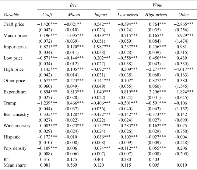
Elasticities derived from the Rotterdam model for the system of six categories of beer and wine are reported in Table 9.Footnote 20 Elasticities are computed at the means of the sample data, and the elasticities with respect to demographic demand shifters can be interpreted as the percentage change in demand for a product in response to a 1% increase of the demand shift variable relative to its mean. The own- and cross-price elasticities are computed mainly as a check on the performance of the model; we are primarily interested in the response to the demand shifters. Since we are modeling allocations of group expenditure, the Marshallian price elasticities in Table 9 are conditional on total expenditure on beer and wine.
Elasticities from the Rotterdam Model Estimated Using DMA-Level Data, 2006–2015

Notes: Marshallian price elasticities and expenditure elasticities, conditional on total beer and wine expenditure. Second-stage estimation.
Source: Created by the authors using data from Nielsen and other sources as described in Table 3.
The model generally performs well, but because the expenditure share of “other wine” is very small, some of the corresponding elasticities and their standard errors in that equation are quite large, and some of the measured effects are not statistically significant—especially among the demographic factors. The own-price elasticities of demand are negative and elastic for each category, consistent with expectations and encouraging us to place some confidence in the performance of the model. The cross-price elasticities suggest that the three beer categories are substitutes for one another (with the exception of macro and imported beer), but we note a few complementarities between some categories of beer and wine, as well as between some wine categories. The estimated expenditure elasticities—reflecting allocation of beer and wine expenditures—are plausible magnitudes and ranked as expected with larger values for craft beer, import beer, high-priced wine, and other wine categories; these groups represent the premium categories, whereas macro beer and low-priced wine are the lower-end categories.
The elasticity with respect to the “Trump” variable indicates that in regions where Trump had greater voter support in the 2016 national election, consumers tend to demand more macro beer, but less of everything else. The responses to the ancestral preference variables are generally consistent with expectations, but with some small surprises in terms of the effects on demand for imported beer and high-priced wine. An increase in the ancestral preference for beer is associated with a decrease or no change in demand for all categories of wine and an increase in demand for macro and craft beer, but a decrease in demand for imported beer. An increase in the ancestral preference for wine is associated with an increase in demand for low-priced wine and a decrease in demand for macro beer, but also increases in demand for craft and imported beer and a decrease in demand for high-priced wine. The increase in the demand for imported beer associated with an increase in the Hispanic share of the population probably reflects a demand by people with Mexican antecedents for the many popular beers imported from Mexico. The population density variable suggests that representative consumers in more urban areas demand more high-priced wine and imported beer, but less craft beer and less low-priced wine.
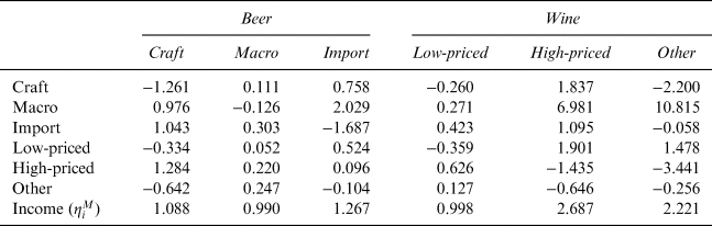
Elasticities of demand for each type of beer and wine with respect to income (total expenditure on all goods) and with respect to prices conditional on income, calculated according to Equations (9) and (10) and, thus, combining the first-stage estimates from Table 8 and the second-stage estimates from Table 9, are reported in Table 10. These elasticities are intuitive.
Marshallian Price and Expenditure Elasticities, Conditional on Total Expenditure

Notes: Marshallian price elasticities and expenditure elasticities, conditional on income. Calculated from first- and second-stage estimates as described in Equations (9) and (10).
Source: Created by the authors using data from Nielsen and other sources as described in Table 3.
VII. Conclusion
Across the United States, populations can differ substantially in terms of their ethnic and cultural background. Looking at the state-level longer-term data (1970–2016), consumption patterns vary significantly spatially in terms of the balance between beer and wine, and are not converging. Furthermore, as revealed by our analysis using more detailed data over a shorter period (2006–2015), the consumption patterns within each alcohol category vary greatly.
In this article, we focused on the role of demographic characteristics of populations as potential determinants of these persistent spatial patterns that could not reasonably be accounted for by conventional economic variables. In doing so, we sought to control for the effects of prices and incomes (or total expenditures) and where possible to obtain useful measures of price and income elasticities. We employed a consistent modeling approach applied to two quite different data sets, which enables us to make some inferences about the consequences of aggregation across consumers, goods, and time for our findings.
First, using state-level annual per capita time series data, we estimated both single equation (logarithmic differential) models of demand and the Rotterdam model, treating alcohol (beer, wine, and spirits) as a weakly separable group. This enabled us to compute elasticities of demand conditional on group expenditure (i.e., alcohol) and elasticities conditional on total expenditure on all goods, as is more relevant for most policy questions. Plots of the data and some pretesting led us to split the data for this analysis into two sub-periods. In this work we were concerned that the measures of prices were seriously inadequate and that there might be further problems occasioned by the aggregation of data across diverse regions within states, and across diverse products within categories. This analysis yielded results that might be seen as plausible at first blush, but the estimates were somewhat fragile and mixed with respect to some of the demographic factors of greatest interest. Ultimately, we concluded that it would be of interest to conduct an analysis using less-aggregative data with better measures of prices.
The results from our analysis using disaggregated data are much more consistent with expectations and are much more satisfactory. We found strong and compelling evidence that ancestral alcohol consumption patterns, urbanization, and political affiliations are associated with differing consumer preferences for types of beer and wine. Considering beer and wine together, areas with populations having stronger ancestral links to beer-drinking nations demand relatively more macro and craft beer compared to other beverages, and less imported beer and low- and high-priced wine. Areas with populations with high ancestral wine consumption demand relatively more craft and imported beer and low-priced wine, and less macro beer and high-priced wine. An increase in the Hispanic share of the population is associated with an increase in demand for imported beer and low-priced wine relative to all other beverages. Areas with more Trump supporters demand more macro beer, but less craft and imported beer and less low- and high-priced wine.
We do not claim causality in any of these findings. We cannot say whether voting for Trump causes Americans to consume more light beer. However, the findings provide compelling evidence that alcohol consumption patterns in the United States are not converging in any simple or general way and the patterns are associated with enduring socioeconomic and demographic characteristics of the population. Total alcohol consumption and shares among categories of alcohol (i.e., beer, wine, and spirits) differ significantly among populations and regions across the country, as do the product shares within alcohol categories. And when we try to explain these differences, it is important to use sufficiently disaggregated data and to look beyond the typical economic variables such as per capita income and prices. Drinking is often tied to culture and tradition, and even after people immigrate to the United States their ancestral beverage preferences persist to some extent and are instilled in younger generations.
Supplementary Material
For supplementary material accompanying this paper visit https://doi.org/10.1017/jwe.2019.14