1 Introduction
Gravity currents are density-driven flows that propagate primarily in the horizontal direction. They play an important role in a host of environmental settings, as well as in a wide range of engineering applications (Simpson Reference Simpson1982; Ungarish Reference Ungarish2009). In constant-density environments, gravity currents commonly advance along top or bottom boundaries. When the ambient density field is stratified, on the other hand, gravity currents can also take the form of intrusions that propagate horizontally at intermediate heights. In geophysical applications, ambient density stratification most often is the result of temperature and salinity variations, such as in lakes and oceans (Sutherland Reference Sutherland2010). The ability of stratified ambients to sustain internal waves can then give rise to a broad range of complex interactions between gravity currents, intrusions and internal waves (Fischer & Smith Reference Fischer and Smith1983; MacIntyre et al. Reference MacIntyre, Flynn, Jellison and Romero1999; Maxworthy et al. Reference Maxworthy, Leilich, Simpson and Meiburg2002; Meiburg & Kneller Reference Meiburg and Kneller2010; Cortés et al. Reference Cortés, Fleenor, Wells, de Vicente and Rueda2014; Hogg Reference Hogg2014; Hogg et al. Reference Hogg, Egan, Ouellette and Koseff2018). Maxworthy et al. (Reference Maxworthy, Leilich, Simpson and Meiburg2002) demonstrated that a gravity current released in a linearly stratified ambient fluid could, under certain circumstances, come to a stop as the waves generated by the release of the current catch up with the head of the current. The entrainment of ambient fluid through turbulent mixing frequently modifies the gravity current density by diluting it, thereby further complicating its dynamics (Ellison & Turner Reference Ellison and Turner1959; Turner Reference Turner1986; Hallworth et al. Reference Hallworth, Huppert, Phillips and Sparks1996; Necker et al. Reference Necker, Härtel, Kleiser and Meiburg2005; Cenedese & Adduce Reference Cenedese and Adduce2010).
When gravity currents flow down a slope within a continuously stratified environment, they typically intrude horizontally at their point of neutral buoyancy (Baines Reference Baines2001; Snow & Sutherland Reference Snow and Sutherland2014; Biegert et al. Reference Biegert, Vowinckel, Ouillon and Meiburg2017). Intrusions at intermediate depths were also observed in the large-scale simulations of Marques et al. (Reference Marques, Wells, Padman and Özgökmen2017), which considered gravity currents propagating downslope into quiescent stratified ambients. The authors found that flow splitting, a process in which partially mixed current fluid forms a horizontal intrusion while denser current fluid continues down the slope as a hyperpycnal current, is susceptible to occur in weakly stratified environments such as Arctic outflows. On the other hand, if the ambient consists of two constant-density layers, with a jump in the density at the interface, and if the current is denser than both of these layers, it will split into a neutrally buoyant intrusion of diluted fluid that propagates along the interface and a hyperpycnal bottom current that continues to move down the slope at a reduced velocity (Samothrakis & Cotel Reference Samothrakis and Cotel2006; Monaghan Reference Monaghan2007; Cortés et al. Reference Cortés, Fleenor, Wells, de Vicente and Rueda2014). Of particular interest in the present context are gravity currents formed by the discharge of concentrated brine from desalination plants (Fernández-Torquemada et al. Reference Fernández-Torquemada, Gónzalez-Correa, Loya, Ferrero, Díaz-Valdés and Sánchez-Lizaso2009; Hodges, Furnans & Kulis Reference Hodges, Furnans and Kulis2011). Understanding the mixing of this brine under the influence of the near-coastal internal wave field, along with its transport into deeper water, is important for assessing its ecological impact on the coastal ocean environment.
Mindful of the importance of internal wave dynamics in limnology (Mortimer Reference Mortimer1952), Fischer & Smith (Reference Fischer and Smith1983) over the course of two 14-day experiments injected dye into a dense stream entering Lake Mead in order to investigate the transport of nutrients. They found substantial amounts of the dye at the lake surface, despite theoretical predictions that the dense fluid from the stream should form a hyperpycnal current intruding at the thermocline. Without providing a detailed explanation, the authors hypothesized that large-amplitude internal waves measured during the experiments might have interacted with the bottom current, thereby modifying the transport of the dense stream fluid.
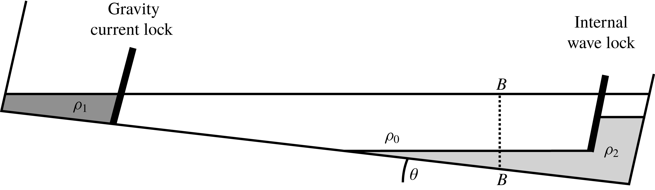
Recent laboratory experiments by Hogg et al. (Reference Hogg, Egan, Ouellette and Koseff2018) have unravelled some of the physics governing gravity current–wave interactions at a density interface. Using the tank apparatus sketched in figure 1, those authors initiated the gravity current and internal wave via lock release, and subsequently studied their collision where the pycnocline meets the slope. Holding the gravity current properties constant, the authors observed a strong reduction of the gravity current mass flux for increasing wave amplitudes. Hogg et al. (Reference Hogg, Egan, Ouellette and Koseff2018) furthermore identified a ‘decapitation’ process by which the internal wave removes part of the gravity current head from its body and transports it upslope. The process differs from both detrainment and entrainment processes expected to take place in a downslope dense flow in the gravity current regime (Baines Reference Baines2008). The gravity current regime is observed in the case of a dense current propagating down a gentle slope and is characterized by detrainment of dense fluid into the ambient and to a lesser extent entrainment of ambient fluid into the current, thus affecting its density (Baines Reference Baines2008). In the experiments of Hogg et al. (Reference Hogg, Egan, Ouellette and Koseff2018), the ambient fluid is stratified with a sharp pycnocline separating two homogeneous layers, such that entrainment affects the proportion of the gravity current fluid forming an intrusion at the density interface. The decapitation process generates mixing between the current fluid and dense ambient fluid through a new mechanism not accounted for by detrainment, entrainment or flow splitting, further motivating a detailed analysis of its dynamics.
The current investigation analyses and quantifies the energetics and mixing dynamics of the above current–wave interaction in depth via direct numerical simulations, and explores its dependence on the governing dimensionless parameters. Section 2 presents the flow configuration and discusses the governing equations, along with the characteristic scales and the computational approach. Section 3 focuses on the analysis of the flow physics, beginning with the gravity current mass flux reduction as a result of the interfacial wave. The splitting of the original gravity current into an intrusion and a hyperpycnal flow is analysed, along with the propagation velocities of the two resulting fronts. The existence of two separate parameter regimes is demonstrated, governed by distinctly different dynamics. A detailed investigation of the decapitation phenomenon follows, particularly with regard to how it contributes to the mixing of the gravity current and ambient fluids. The implications of the current–wave interaction for the various components of the overall energy budget are discussed, including viscous dissipation. Finally, the loss of available potential energy as a result of the irreversible mixing associated with the current–wave interaction is quantified. Section 4 summarizes the key findings and presents the main conclusions of the work.
Schematic of the apparatus employed in the experiments of Hogg et al. (Reference Hogg, Egan, Ouellette and Koseff2018). Both the gravity current and the internal wave are initiated via lock release. The vertical interrogation plane is shown by the dotted line.

2 Numerical set-up and governing equations
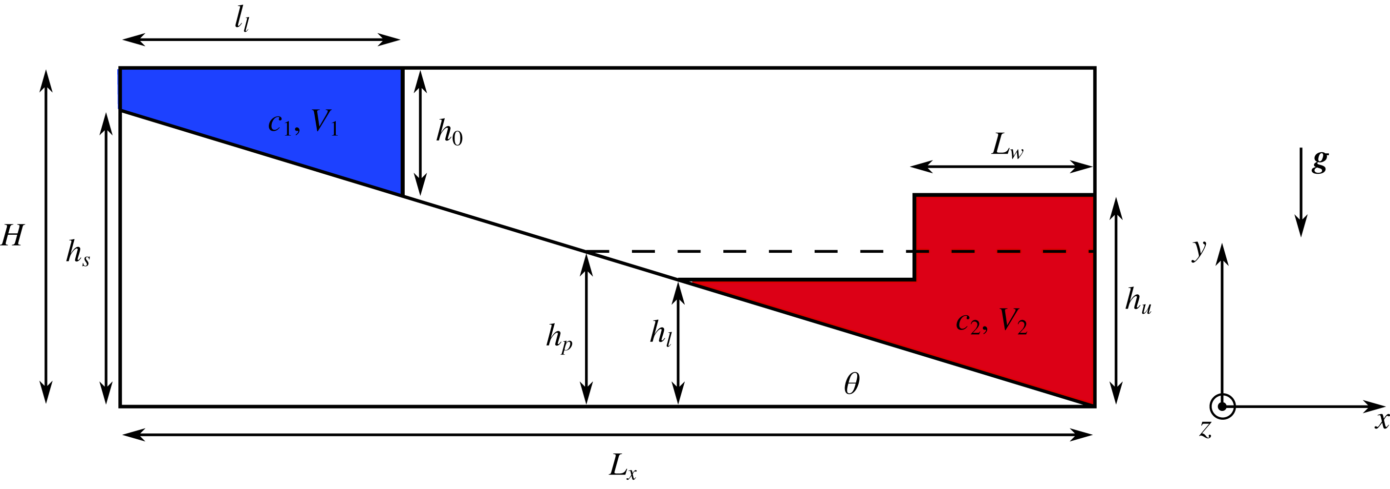
The initial configuration of the simulations is shown in figure 2. A lock with scalar concentration
 $c_{1}$
and volume
 $V_{1}$
is separated from the ambient by a virtual gate. The lower, denser region of the two-layer ambient has an initial scalar concentration
 $c_{2}$
and volume
 $V_{2}$
, while there is no scalar in the upper ambient region. The denser ambient is raised to a height
 $h_{u}$
over a length
 $l_{w}$
from the right-hand wall whilst keeping the volume
 $V_{2}$
constant, causing the left-hand part of the ambient to be lowered to height
 $h_{l}$
. The height difference between the two parts of the dense ambient is
 $h_{w}=h_{u}-h_{l}$
. The ratio of wave height to wavelength
 $h_{w}/l_{w}$
is referred to as the wave Froude number
 $Fr$
(Hogg et al.
Reference Hogg, Egan, Ouellette and Koseff2018). This definition of the Froude number follows from the classical definition
 $U_{w}/\sqrt{g_{w}^{\prime }h_{w}}$
, where
 $U_{w}$
denotes the wave speed and
 $g_{w}^{\prime }=g(\unicode[STIX]{x1D70C}_{2}-\unicode[STIX]{x1D70C}_{0}/\unicode[STIX]{x1D70C}_{0})$
, and involves using scales appropriate to the experimental set-up. From wave theory we can show that
 $U_{w}\sim h_{w}\unicode[STIX]{x1D714}$
, where
 $\unicode[STIX]{x1D714}$
is the wave frequency, and
 $\unicode[STIX]{x1D714}\sim \sqrt{h_{w}/D}$
, where
 $D$
is the depth of the dense fluid from the two-layer interface to the bottom floor. Since
 $D$
is not constant but rather changes in space as the wave propagates, we use
 $l_{w}$
which is comparable to
 $D$
in the experiments, and which reflects the wavelength of the released wave. Given that
 $l_{w}$
is a reasonable surrogate for the depth, then
 $U_{w}\sim h_{w}\sqrt{g_{w}^{\prime }/l_{w}}$
. The celerity associated with the wave propagation then becomes
 $c\approx \sqrt{g_{w}^{\prime }l_{w}}$
. Substituting all of this into the definition of the wave Froude number thus gives us
 $U_{w}/c\sim h_{w}\sqrt{g_{w}^{\prime }/l_{w}}/\sqrt{g_{w}^{\prime }l_{w}}=h_{w}/l_{w}$
.
Initial set-up for studying the interaction between a lock-release gravity current and an interfacial wave. Here
 $c_{1}=1$
and
 $c_{2}<1$
are the initial concentrations of the lock fluid and the dense ambient fluid, respectively;
 $V_{1}$
and
 $V_{2}$
indicate the volumes of lock fluid and dense ambient fluid. At
 $t=0$
the lock is released and the gravity current begins to move down the slope. At
 $t=t_{1}$
the wave lock is released and the wave starts propagating towards the slope.

2.1 Dimensional governing equations
We solve the three-dimensional, unsteady Navier–Stokes equations for incompressible flows in the Boussinesq limit, since density changes due to salt or temperature variations are typically small in applications of interest. The scalar concentration field is governed by an advection–diffusion equation. The dimensional equations are given by
 $$\begin{eqnarray}\displaystyle & \displaystyle \unicode[STIX]{x1D735}\boldsymbol{\cdot }\boldsymbol{u}=0, & \displaystyle\end{eqnarray}$$
 $$\begin{eqnarray}\displaystyle & \displaystyle \frac{\unicode[STIX]{x2202}\boldsymbol{u}}{\unicode[STIX]{x2202}t}+(\boldsymbol{u}\boldsymbol{\cdot }\unicode[STIX]{x1D735})\boldsymbol{u}=-\frac{1}{\unicode[STIX]{x1D70C}_{0}}\unicode[STIX]{x1D735}p+\unicode[STIX]{x1D708}\unicode[STIX]{x0394}\boldsymbol{u}+\frac{\unicode[STIX]{x1D70C}-\unicode[STIX]{x1D70C}_{0}}{\unicode[STIX]{x1D70C}_{0}}\boldsymbol{g}, & \displaystyle\end{eqnarray}$$
 $$\begin{eqnarray}\displaystyle & \displaystyle \frac{\unicode[STIX]{x2202}c_{i}}{\unicode[STIX]{x2202}t}+\boldsymbol{u}\boldsymbol{\cdot }\unicode[STIX]{x1D735}c_{i}=\unicode[STIX]{x1D705}_{c}\unicode[STIX]{x0394}c_{i},\quad i=\{c,w\}, & \displaystyle\end{eqnarray}$$
where
 $\boldsymbol{u}$
denotes the velocity vector,
 $p$
represents pressure,
 $\unicode[STIX]{x1D70C}$
indicates the local density with the freshwater density
 $\unicode[STIX]{x1D70C}_{0}$
serving as a reference value and
 $c_{c}$
and
 $c_{w}$
are the salinity concentrations of the current and wave fluid, respectively. Note that two distinct scalar fields are defined for the current and ambient salinities, so that we can easily keep track of each fluid, similarly to what is accomplished in the experiments by adding dyes. The kinematic viscosity of water is assumed to be constant at
 $\unicode[STIX]{x1D708}=10^{-6}~\text{m}^{2}~\text{s}^{-1}$
. Since the influence of the scalar diffusivity
 $\unicode[STIX]{x1D705}_{c}$
on the propagation velocity of a gravity current is small as long as
 $\unicode[STIX]{x1D705}_{c}\leqslant \unicode[STIX]{x1D708}$
, we choose
 $\unicode[STIX]{x1D705}_{c}=\unicode[STIX]{x1D708}$
for simplicity (Härtel, Meiburg & Necker Reference Härtel, Meiburg and Necker2000; Necker et al.
Reference Necker, Härtel, Kleiser and Meiburg2005; Cantero et al.
Reference Cantero, Balachandar, García and Bock2008). How this assumption might affect long-term observations of irreversible mixing in the flow will be discussed in § 3.5. The gravitational acceleration is given by
 $\boldsymbol{g}=-g\boldsymbol{e}_{y}$
. The density depends linearly on the salinity such that
 $$\begin{eqnarray}\displaystyle \unicode[STIX]{x1D70C}=\unicode[STIX]{x1D70C}_{0}(1+\unicode[STIX]{x1D6FC}c_{c}+\unicode[STIX]{x1D6FC}c_{w}), & & \displaystyle\end{eqnarray}$$
where
 $\unicode[STIX]{x1D6FC}=\unicode[STIX]{x2202}\unicode[STIX]{x1D70C}/\unicode[STIX]{x2202}c=\text{const.}$
denotes the expansion coefficient.
2.2 Characteristic quantities and non-dimensional equations
The lock height
 $h_{0}$
is used as a reference length, since it directly affects the propagation velocity of the gravity current. The reference concentration is chosen as the initial concentration of the lock
 $c_{c}(t=0)=c_{1}$
. A buoyancy velocity based on the initial density difference between the lock and the ambient fluid is used to define the velocity scale:
 $$\begin{eqnarray}\displaystyle u_{b}=\sqrt{\frac{\unicode[STIX]{x1D70C}_{1}-\unicode[STIX]{x1D70C}_{0}}{\unicode[STIX]{x1D70C}_{0}}gh_{0}}, & & \displaystyle\end{eqnarray}$$
where
 $\unicode[STIX]{x1D70C}_{1}=\unicode[STIX]{x1D70C}_{0}(1+\unicode[STIX]{x1D6FC}c_{1})$
is the density of the gravity current fluid initially contained behind the lock and
 $\unicode[STIX]{x1D70C}_{0}$
is the density of the upper ambient fluid (figure 1). This defines our reference time scale
 $T=h_{0}/u_{b}$
. The dimensional variables (left) are then made non-dimensional (right) as follows:
 $$\begin{eqnarray}\displaystyle & \displaystyle \boldsymbol{x}\rightarrow \boldsymbol{x}h_{0}, & \displaystyle\end{eqnarray}$$
 $$\begin{eqnarray}\displaystyle & \displaystyle \boldsymbol{u}\rightarrow \boldsymbol{u}u_{b}, & \displaystyle\end{eqnarray}$$
 $$\begin{eqnarray}\displaystyle & \displaystyle t\rightarrow tT, & \displaystyle\end{eqnarray}$$
 $$\begin{eqnarray}\displaystyle & \displaystyle p\rightarrow p\unicode[STIX]{x1D70C}_{0}u_{b}^{2}, & \displaystyle\end{eqnarray}$$
 $$\begin{eqnarray}\displaystyle & \displaystyle c_{i}\rightarrow c_{i}c_{1},\quad i=\{c,w\}. & \displaystyle\end{eqnarray}$$
This yields the non-dimensional form of the governing equations
 $$\begin{eqnarray}\displaystyle & \displaystyle \unicode[STIX]{x1D735}\boldsymbol{\cdot }\boldsymbol{u}=0, & \displaystyle\end{eqnarray}$$
 $$\begin{eqnarray}\displaystyle & \displaystyle \frac{\unicode[STIX]{x2202}\boldsymbol{u}}{\unicode[STIX]{x2202}t}+(\boldsymbol{u}\boldsymbol{\cdot }\unicode[STIX]{x1D735})\boldsymbol{u}=-\unicode[STIX]{x1D735}p+\frac{1}{Re}\unicode[STIX]{x0394}\boldsymbol{u}-(c_{c}+c_{w})\boldsymbol{e}_{y}, & \displaystyle\end{eqnarray}$$
 $$\begin{eqnarray}\displaystyle & \displaystyle \frac{\unicode[STIX]{x2202}c_{i}}{\unicode[STIX]{x2202}t}+\boldsymbol{u}\boldsymbol{\cdot }\unicode[STIX]{x1D735}c_{i}=\frac{1}{Pe}\unicode[STIX]{x0394}c_{i},\quad i=c,w, & \displaystyle\end{eqnarray}$$
where
 $Re=(u_{b}h_{0}/\unicode[STIX]{x1D708})$
is the Reynolds number and
 $Pe=ReSc$
is the Peclet number, with
 $Sc=(\unicode[STIX]{x1D708}/\unicode[STIX]{x1D705}_{c})$
being the Schmidt number. As mentioned previously, the Schmidt number is set to unity. Slip boundary conditions are employed at the top and right-hand walls, and periodic conditions are used in the spanwise direction. No-slip conditions are applied at the left-hand wall and on the slope (
 $\boldsymbol{u}_{\mid \unicode[STIX]{x1D6E4}_{s}}=0$
). The width
 $L_{z}/H=0.2$
of the domain is chosen sufficiently large so that the three-dimensional lobe and cleft instability can develop in the spanwise direction. No-flux boundary conditions are applied at all boundaries for the salinity.
2.3 Numerical method
The equations are solved by our direct immersed boundary method code, originally developed under the name TURBINS (Nasr-Azadani & Meiburg Reference Nasr-Azadani and Meiburg2011). The immersed boundary method is employed to impose the no-slip condition on the slope (Mittal & Iaccarino Reference Mittal and Iaccarino2005; Kang Reference Kang2008; Nasr-Azadani & Meiburg Reference Nasr-Azadani and Meiburg2011). A small random perturbation is added to the
 $u$
-component of the velocity field at
 $t=0$
, in order to facilitate the three-dimensional evolution of the flow. The computational domain is discretized by
 $(N_{x}\times N_{y}\times N_{z})=(3000\times 300\times 30)$
cells, corresponding to a grid size of
 $\unicode[STIX]{x0394}x/H=\unicode[STIX]{x0394}y/H=\unicode[STIX]{x0394}z/2H=0.0033$
. The higher resolution in the
 $x,y$
-plane is employed to ensure mass conservation at the immersed boundary.
3 Results
3.1 Simulation parameters
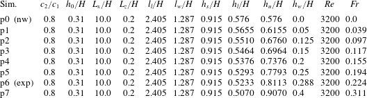
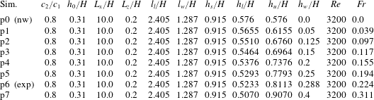
We conduct direct numerical simulations for the dimensionless parameter combinations listed in tables 1 and 2. Table 1 describes the simulations conducted to investigate the evolution of mass flux with wave height, while keeping the lower pycnocline at a constant vertical position
 $h_{l}/H=0.568$
. This is done to guarantee that the mass flux interrogation planes are equally distant from the point of contact between the slope and the pycnocline across simulations. Table 2 describes the parametric study of the influence of the wave height on the current–wave interaction. In these simulations the volume of the dense ambient is kept constant, in order to keep the initial background potential energy constant (cf. the discussion in § 3.4). Simulation p6 corresponds precisely to the experimental configuration of Hogg et al. (Reference Hogg, Egan, Ouellette and Koseff2018).
Simulation parameters employed to investigate the influence of the dimensionless wave height on the current fluid mass flux. Here (nw) denotes the absence of a wave.

Simulation parameters employed to investigate the influence of the dimensionless wave height on the current–wave interaction. Simulation p6 precisely reproduces the experimental set-up. The no-wave case (nw) of simulation p0 serves as reference case for quantifying the effect of the wave on mixing.
3.2 Mass flux
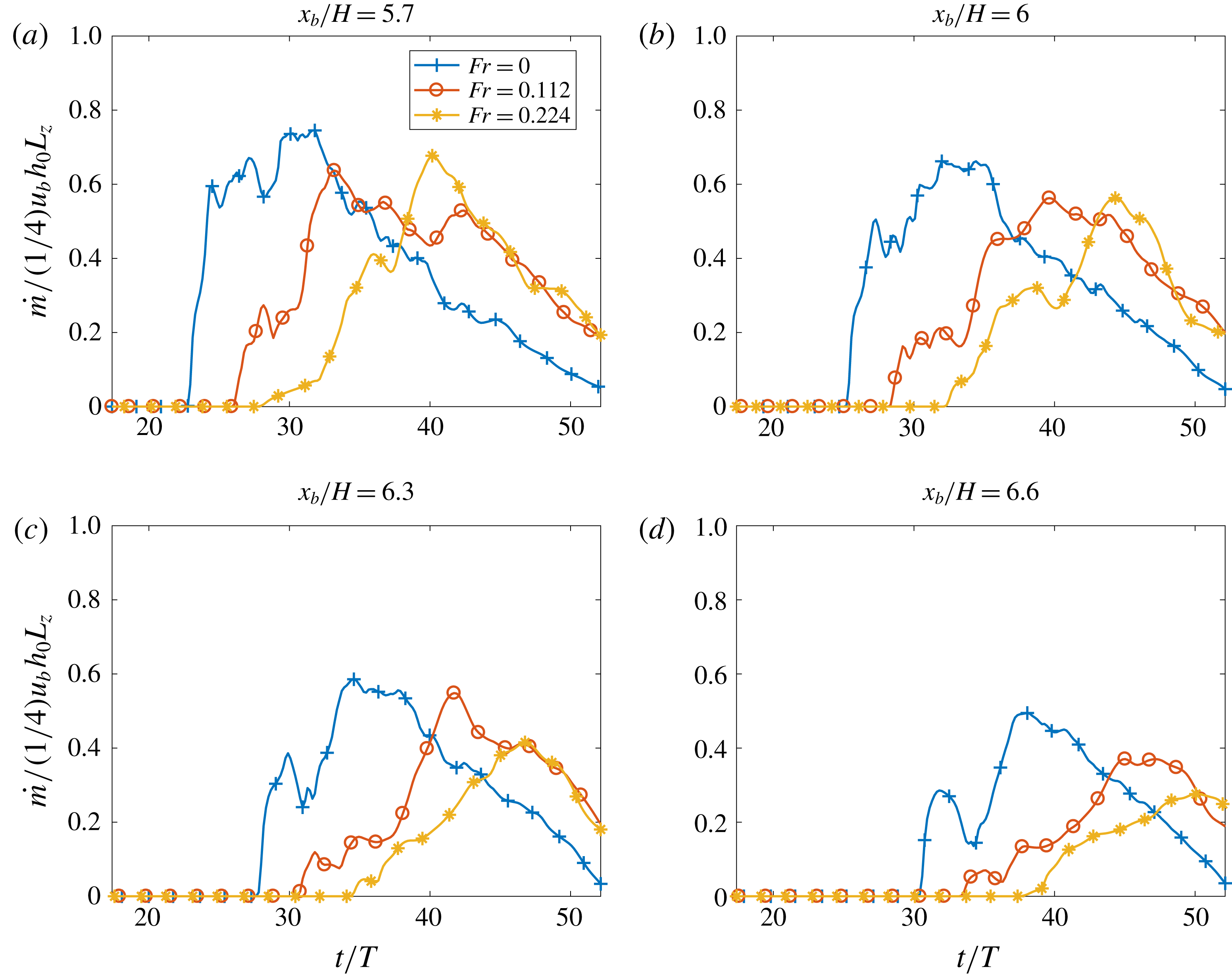
In the following, we compare gravity current mass flux data with corresponding experimental results of Hogg et al. (Reference Hogg, Egan, Ouellette and Koseff2018). Towards this end, we calculate the spanwise-averaged mass flux of gravity current fluid at the four interrogation planes
 $x_{b}/H=5.7$
, 6.0, 6.3 and 6.6, as shown in figure 3. These locations correspond to points on the slope below the ambient pycnocline, so that the mass flux data capture both the fraction of the gravity current fluid which has penetrated through the pycnocline, as well as the fraction that is transported as an intrusion along the pycnocline. Given the statistically two-dimensional nature of the flow, this corresponds to taking ensemble averages. The mass flux is thus calculated as
 $$\begin{eqnarray}\displaystyle {\dot{m}}=\int _{0}^{L_{z}}\int _{y_{s}(x_{b})}^{H}uc_{c}\,\text{d}y\,\text{d}z, & & \displaystyle\end{eqnarray}$$
where
 $y_{s}(x_{b})$
indicates the vertical coordinate of the slope at the location
 $x_{b}$
of the interrogation plane. We normalize the mass flux based on the observation that a lock-exchange gravity current propagating on a flat surface has a height close to half the lock height, and a front velocity
 $U_{f}\approx (1/2)u_{b}$
during the slumping phase (Benjamin Reference Benjamin1968; Huppert & Simpson Reference Huppert and Simpson1980; Shin, Dalziel & Linden Reference Shin, Dalziel and Linden2004; Borden & Meiburg Reference Borden and Meiburg2013).
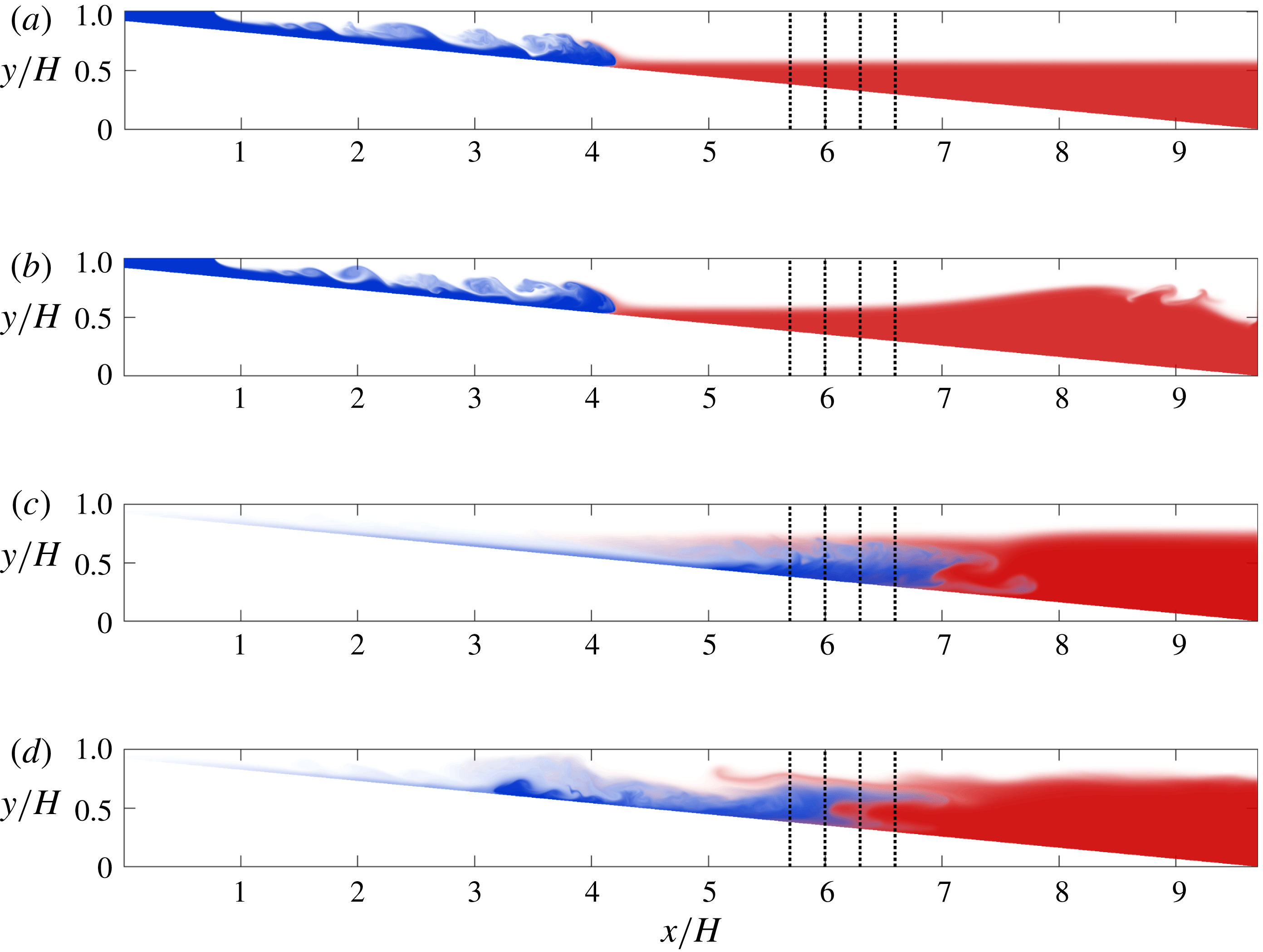
Snapshots of the gravity current concentration
 $c_{c}$
(blue) superimposed with the lower ambient fluid concentration
 $c_{w}$
(red) at
 $t/T=12.17$
(a,b) and
 $t/T=43.45$
(c,d) without (a,c) and with (b,d) an incoming wave (
 $Fr=0.224$
). The gravity current begins to interact with the dense bottom layer even before the wave reaches the slope. The dashed vertical lines correspond to the locations
 $x=x_{b}$
where the mass flux is evaluated.

Normalized mass flux data are shown as functions of time in figure 4. Further upstream interrogation planes see higher peak mass fluxes, which reflects the significant slowdown of the gravity current as it encounters the dense lower ambient fluid. The presence of a wave reduces the mass flux, consistent with the observations of Hogg et al. (Reference Hogg, Egan, Ouellette and Koseff2018).
Mass flux as a function of time at interogation planes (a)
 $x_{f}/H=5.7$
, (b)
 $x_{f}/H=6$
, (c)
 $x_{f}/H=6.3$
and (d)
 $x_{f}/H=6.6$
. All locations are past the point where the pycnocline reaches the slope, and therefore reflect the ability of the current to penetrate the pycnocline for various wave sizes. The transport of gravity current fluid is both reduced and delayed by the wave.

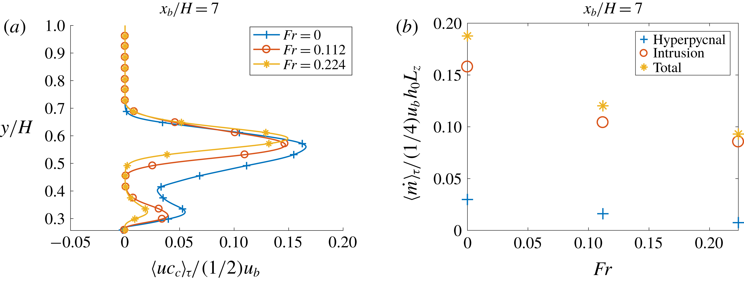
Figure 4 furthermore indicates that the arrival of the gravity current fluid at the interrogation planes is delayed in the presence of a large wave. The energetics of this process will be analysed in detail below. To distinguish the hyperpycnal component of the gravity current mass flux from the intrusion component, we calculate the time-averaged value
 $\langle uc_{c}(y)\rangle _{\unicode[STIX]{x1D70F}}$
over the averaging window
 $\unicode[STIX]{x1D70F}\in [t_{p},t_{end}]$
at
 $x_{b}=7$
. Here,
 $t_{p}$
corresponds to the time at which the current reaches the interrogation plane and
 $t_{end}$
is chosen so as to avoid any influence from waves reflected by the right-hand boundary of the computational domain. The profiles shown in figure 5(a) exhibit two maxima, one close to the slope and the other near the pycnocline. The former is associated with the hyperpycnal current component, while the latter reflects the intrusion part. The simulations indicate that both with and without a wave, the gravity current fluid transport is dominated by the intrusion component. Consistent with the observations of Hogg et al. (Reference Hogg, Egan, Ouellette and Koseff2018), large waves are found to reduce the hyperpycnal flux component substantially. By associating the mass flux above (below) the local minimum in the vertical profile with the intrusion (hyperpycnal current), we can quantify the two components. The results shown in figure 5(b) confirm that for the present density ratio of
 $c_{2}/c_{1}=0.8$
, the gravity current fluid transport is dominated by the intrusion. The horizontal distance between the lock and the point of interaction at the pycnocline controls the amount of entrainment that occurs within the current and will therefore have an impact on the proportion of fluid that forms the intrusion. This distance is kept constant in the mass-flux simulations and thus the entrainment prior to reaching the pycnocline remains the same across simulations, thus isolating the effect of the wave in the mass-flux calculations. Furthermore, it is evident that both the intrusive and the hyperpycnal components are reduced by the wave. Hogg et al. (Reference Hogg, Egan, Ouellette and Koseff2018) observed a reduction of the mass flux of up to
 $40\,\%$
for a wave with Froude number
 $Fr=0.224$
. The present simulations yield comparable values of
 $36\,\%$
(
 $Fr=0.112$
) and
 $50\,\%$
(
 $Fr=0.224$
) for the total mass flux. For the hyperpycnal component only, reductions of
 $45\,\%$
and
 $75\,\%$
are obtained. Thus, the current–wave interaction not only changes the overall mass flux of the gravity current into the ambient fluid, but it also redistributes these fluxes towards the intrusion. The change in mass flux depends strongly on the timing of the wave release, i.e. on
 $t_{1}-t_{0}$
. The effect of
 $t_{1}$
is not analysed systematically in this numerical study as it was previously explored in the experimental work of Hogg et al. (Reference Hogg, Egan, Ouellette and Koseff2018). In the experiments, the timing was adjusted to yield a maximum effect of the wave on the propagation of the current, and the value of
 $t_{1}-t_{0}$
was replicated directly in the simulations. In order to obtain insight into the mechanisms responsible for these observations, we will in the following focus on the detailed dynamics of the current–wave interaction, including its energetics.
(a) Time-averaged profile of the horizontal flux of gravity current fluid
 $uc_{c}$
as a function of
 $y$
. (b) Discrete contributions of the hyperpycnal and intrusive gravity current to the total time-averaged mass flux as a function of the wave Froude number. The averaging window is
 $t/T\in [t_{p}/T,52.14]$
, i.e from the beginning of the intrusion to the end of the numerical simulation.

3.3 The decapitation phenomenon
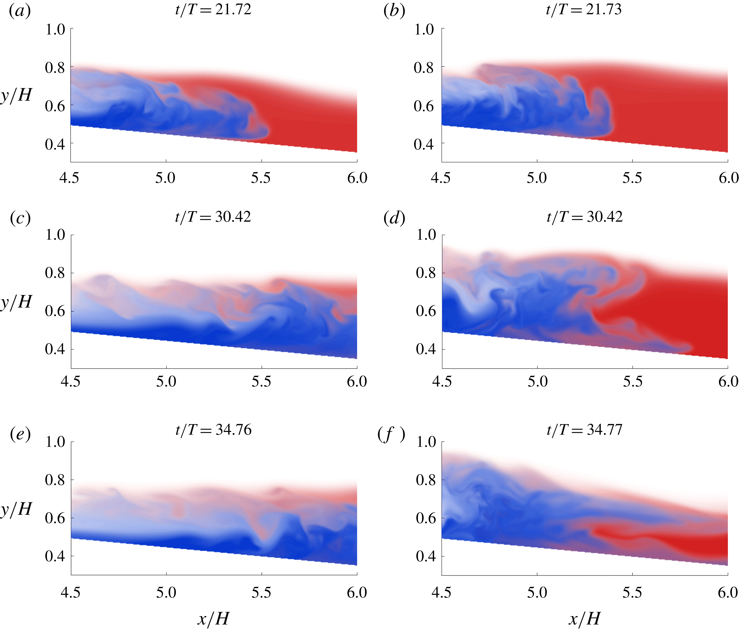
A striking feature of the current–wave interaction brought to light by the experiments of Hogg et al. (Reference Hogg, Egan, Ouellette and Koseff2018) occurs when the current and the wave arrive simultaneously at the location where the pycnocline meets the slope, as shown in figure 6. As the current and the wave collide, the head of the current slows to a halt and lifts off the slope. A fraction of the horizontal momentum carried by the wave and the current is converted into vertical momentum, and part of the current is reflected upslope. The remainder of the current’s body regenerates a head and continues moving downslope as a hyperpycnal current, while partially mixed gravity current fluid forms an intrusion that propagates horizontally along the pycnocline. The distinction between the hyperpycnal component and intrusive flow is most obvious some distance downslope from the initial point of interaction, as seen in figure 6. Due to inertia, the current is initially able to penetrate past the pycnocline before separation occurs. This complex interaction mechanism occurs only for sufficiently large waves, whereas for smaller waves the current merely slows down while retaining its initial head shape. This reflects the strong dependence of the current–wave interaction and the associated mixing on the wave height.
Snapshots of the gravity current concentration
 $c_{c}$
superimposed with the lower ambient fluid concentration
 $c_{w}$
at various times. Results are shown without (a,c,e) and with (b,d,f) an incoming wave at
 $Fr=0.224$
. In the presence of a strong wave (b,d,f) the gravity current head lifts off the slope and is partially reflected upstream.

Closer inspection of the flow field at the location of the current–wave interaction reveals a key dynamic of the decapitation process. In the absence of a wave, the current pierces the pycnocline and maintains its downslope direction, although it loses some of its forward momentum. Strong entrainment and mixing take place along the sheared interface between the current and the ambient. This mixed fluid subsequently forms an intrusion that propagates horizontally in the ambient, as observed in figure 3(c). Note that while the initial concentration
 $c_{w}(t=0)=c_{2}$
in the lower part of the ambient is smaller than that of the lock
 $c_{c}(t=0)=c_{1}$
, with
 $c_{2}/c_{1}=0.8$
, strong mixing has reduced the concentration of the current head by the time it reaches the pycnocline.
In the presence of a strong wave, this picture changes markedly. Upon contact with the wave at
 $t/T=22.60$
, much of the gravity current head is lifted from the slope. A strong recirculation zone forms behind the head, and the current fluid splits into a downslope hyperpycnal flow, an upstream-propagating reflected current and an intrusion that moves along the pycnocline. The long-term evolution is observed in figure 3(d).
Figure 6 hence demonstrates that the dynamics of the current front is strongly altered by the interaction process. As described by Hogg et al. (Reference Hogg, Egan, Ouellette and Koseff2018), the original head of the hyperpycnal current is lifted upwards by the wave, and a new current front subsequently forms from the body of the current. In order to quantify the resulting delayed progression of the hyperpycnal flow below the pycnocline, we define the front location
 $x_{f}$
as the rightmost horizontal position at which
 $$\begin{eqnarray}\displaystyle c_{c}(x,y)\geqslant c_{t}, & & \displaystyle\end{eqnarray}$$
where we choose
 $c_{t}=0.1$
, although the observations to be discussed in the following do not vary significantly with
 $c_{t}$
. Regardless of whether a wave is present or not, the gravity current splits into an intrusion flow along
 $y=h_{p}$
and a bottom-propagating hyperpycnal component. We can identify the hyperpycnal and intrusion front locations at time
 $t$
as follows. First, we determine
 $x_{f}(y)$
for all
 $y$
-values. Subsequently we evaluate the slope height
 $y_{s}(x_{f})$
for each value
 $x_{f}(y)$
. The two front locations are then defined as
 $$\begin{eqnarray}\displaystyle x_{f}=\left\{\begin{array}{@{}l@{}}\max (x_{f}(y)),\quad \forall y\leqslant y_{s}(x_{f})+\unicode[STIX]{x1D6FF}\text{ (hyperpycnal)},\quad \\ \max (x_{f}(y)),\quad \forall y\geqslant y_{s}(x_{f})+\unicode[STIX]{x1D6FF}\text{ (intrusion)},\quad \end{array}\right. & & \displaystyle\end{eqnarray}$$
where
 $\unicode[STIX]{x1D6FF}$
is sufficiently large to encompass the hyperpycnal bottom-propagating flow, but small enough not to capture the intrusion. The intrusion occurs around
 $h_{p}/H=0.576$
and the hyperpycnal flow reaches depths of
 $y/H\leqslant 0.5$
rapidly after piercing the pycnocline, suggesting that an appropriate value is
 $\unicode[STIX]{x1D6FF}/H=0.1$
. We note that within the range
 $0.05\leqslant \unicode[STIX]{x1D6FF}/H\leqslant 0.15$
the results are not sensitive to the precise value of
 $\unicode[STIX]{x1D6FF}/H$
.
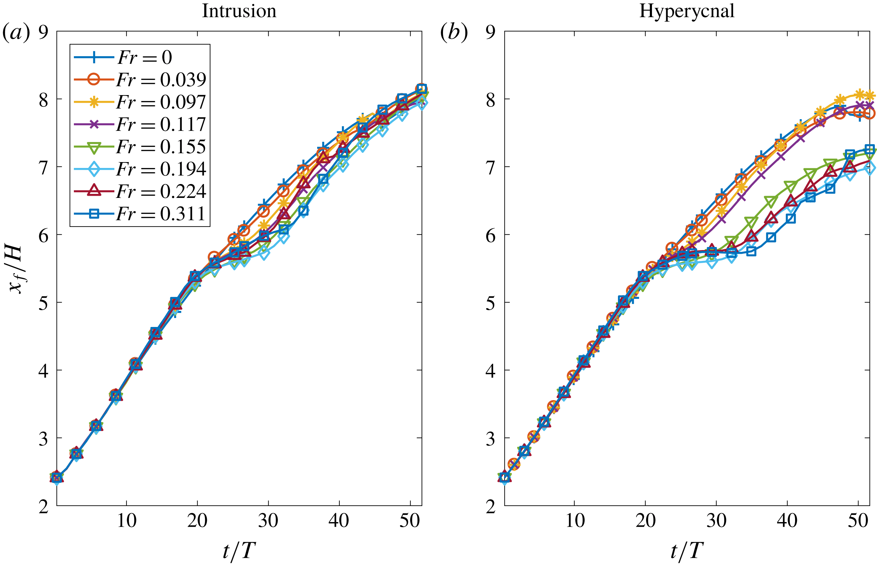
Figure 7 displays both front locations as functions of time. As the wave begins to interact with the current at
 $t/T\approx 20$
, both components of the front abruptly slow down. This slowdown occurs systematically at
 $x/H\approx 5.5$
, defining the horizontal location where the wave–current interaction occurs, and where the intrusion and hyperpycnal components of the current become distinguishable. Subsequently the intrusion front re-accelerates, and for long times its location becomes nearly independent of the wave height. The fast-moving, leftward-propagating wave fluid forces the rightward-propagating intrusion to accelerate, thereby reducing the long-time influence of
 $Fr$
on the intrusion front location. The hyperpycnal front behaves quite differently. For small-amplitude waves with
 $Fr<0.155$
, the wave affects the front location only weakly, and the hyperpycnal and intrusion fronts propagate at similar speeds. For large-amplitude waves with
 $Fr\geqslant 0.155$
, the hyperpycnal front comes to a nearly complete stop for a period of
 $t/T\approx 10$
, before it eventually accelerates again. This reflects the decapitation of the original front, and the formation of a new front from the body of the current as described by Hogg et al. (Reference Hogg, Egan, Ouellette and Koseff2018). This dependence of the front propagation velocity on the wave height is consistent with the observation that the decapitation process exists only for sufficiently large waves with
 $Fr\geqslant 0.155$
.
Current front location as function of time for various wave heights. During its interaction with the wave, the initial gravity current front splits into an intrusion front (a) and a hyperpycnal front (b). For large waves with
 $Fr\geqslant 0.155$
, the hyperpycnal front comes to a near-complete stop and then re-accelerates, without ever catching up again with the no-wave case. In contrast, the intrusion front is slowed only temporarily by the wave.

3.4 Energy budget of the current–wave interaction
We now proceed to analyse how the two different current–wave interaction regimes are reflected in the various energy budget components and their temporal evolution; cf. Härtel et al. (Reference Härtel, Meiburg and Necker2000) for a detailed derivation. The potential energy
 $E_{p}$
of the flow is the sum of the contributions from the gravity current and wave scalar fields:
 $$\begin{eqnarray}\displaystyle E_{p}(t)=E_{p,c}(t)+E_{p,w}(t), & & \displaystyle\end{eqnarray}$$
where
 $$\begin{eqnarray}\displaystyle E_{p,c}(t)=\int _{\unicode[STIX]{x1D6FA}}yc_{c}\,\text{d}V\quad \text{and}\quad E_{p,w}(t)=\int _{\unicode[STIX]{x1D6FA}}yc_{w}\,\text{d}V. & & \displaystyle\end{eqnarray}$$
The total kinetic energy
 $E_{k}$
is obtained as
 $$\begin{eqnarray}\displaystyle E_{k}(t)=\int _{\unicode[STIX]{x1D6FA}}\frac{1}{2}u_{i}u_{i}\,\text{d}V, & & \displaystyle\end{eqnarray}$$
while losses due to viscous dissipation from the start of the flow up to time
 $t$
are given by
 $$\begin{eqnarray}\displaystyle L(t)=\int _{t}\unicode[STIX]{x1D716}(t)\,\text{d}t=-\int _{t}\int _{\unicode[STIX]{x1D6FA}}\frac{2}{Re}\unicode[STIX]{x1D634}_{ij}\unicode[STIX]{x1D634}_{ij}\,\text{d}V\,\text{d}t. & & \displaystyle\end{eqnarray}$$
Here
 $\unicode[STIX]{x1D716}(t)$
denotes the volume integral over the dissipation rate and
 $\unicode[STIX]{x1D634}_{ij}$
indicates the rate of strain tensor
 $\unicode[STIX]{x1D634}_{ij}=(1/2)((\unicode[STIX]{x2202}u_{i}/\unicode[STIX]{x2202}x_{j})+(\unicode[STIX]{x2202}u_{j}/\unicode[STIX]{x2202}x_{i}))$
. In the limit of small vertical diffusion fluxes (Winters et al.
Reference Winters, Lombard, Riley and D’Asaro1995), energy conservation implies
 $$\begin{eqnarray}\displaystyle E_{p,c}+E_{p,w}+E_{k}+L=\text{const.} & & \displaystyle\end{eqnarray}$$
In the limit of no mixing, the state of minimal potential energy corresponds to the configuration where the gravity current fluid collects at the bottom of the flow field, with the lower layer ambient fluid placed immediately above. The upper ambient freshwater layer occupies the topmost region. The potential energy of this configuration is a function only of the initial volume and concentration of each fluid region. In order to be able to make meaningful comparisons between different simulations we hence keep these parameters constant between different simulations, by lowering the ambient pycnocline as we increase the wave height.
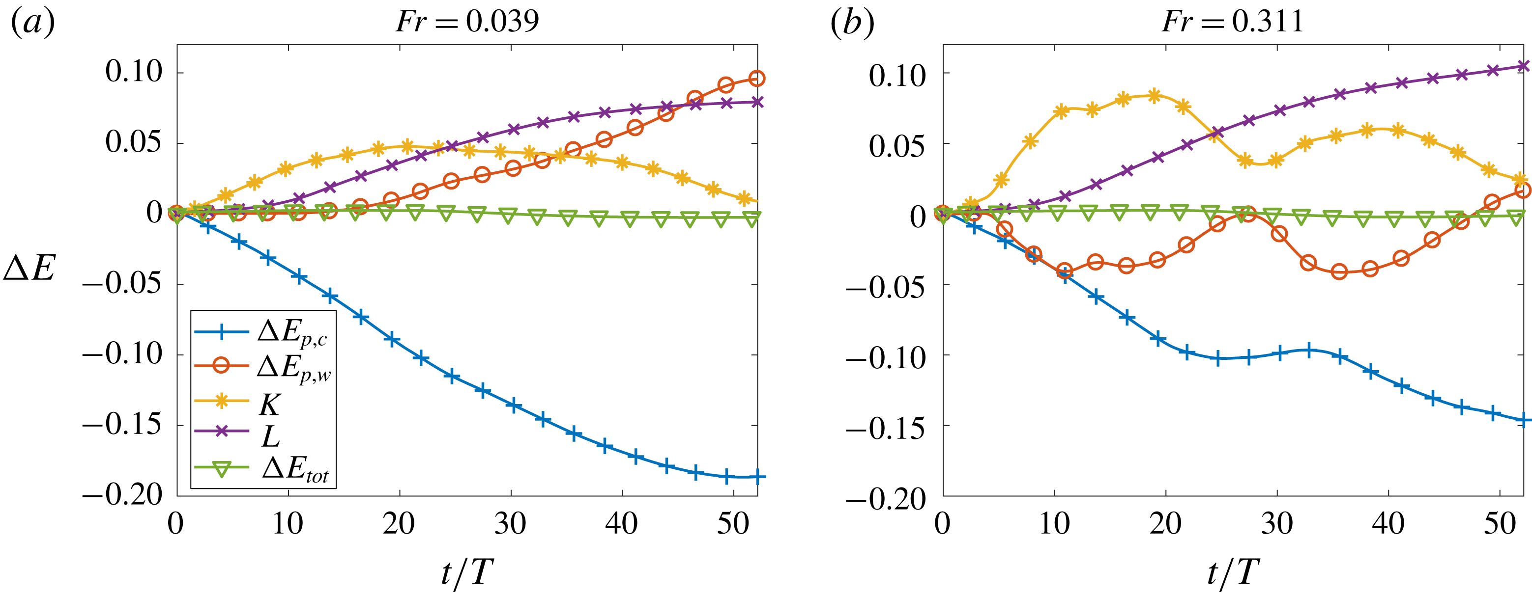
The energy budget components are displayed as functions of time in figure 8, for two different wave heights. Upon release of the lock, the potential energy of the current fluid is converted into kinetic energy, and viscous losses accumulate. As the current pierces the pycnocline in the absence of a wave, a fraction of its kinetic energy is used to lift dense ambient fluid, so that the overall kinetic energy of the flow peaks and then steadily declines. This picture changes in the presence of a wave. While the release of the wave at time
 $t_{1}>0$
initially increases the overall kinetic energy, we note that the horizontal momenta of the current and wave fluid point in opposite directions. As a result, when the current and the wave collide the kinetic energy drops significantly, while the potential energy decrease of the current fluid is temporarily delayed and, for sufficiently large waves, even reversed. This is a direct manifestation of the decapitation process, and of the formation of a reflected, upslope-propagating current. Eventually, however, the potential energy release of the current fluid resumes.
Global energy budget of the current–wave interaction for two wave sizes and their corresponding wave Froude number
 $Fr=h_{w}/l_{w}$
. As the wave height increases, more potential energy is released from the dense ambient fluid, impacting the production of kinetic energy, and modifying the release of potential energy of the gravity current during the current–wave interaction.

The change in the potential energy of the gravity current fluid as a function of time is given by
 $$\begin{eqnarray}\displaystyle \unicode[STIX]{x0394}E_{p,c}(t)=E_{p,c}(t)-E_{p,c}(0). & & \displaystyle\end{eqnarray}$$
The work performed by the wave in order to raise the potential energy of the current fluid can then be obtained as
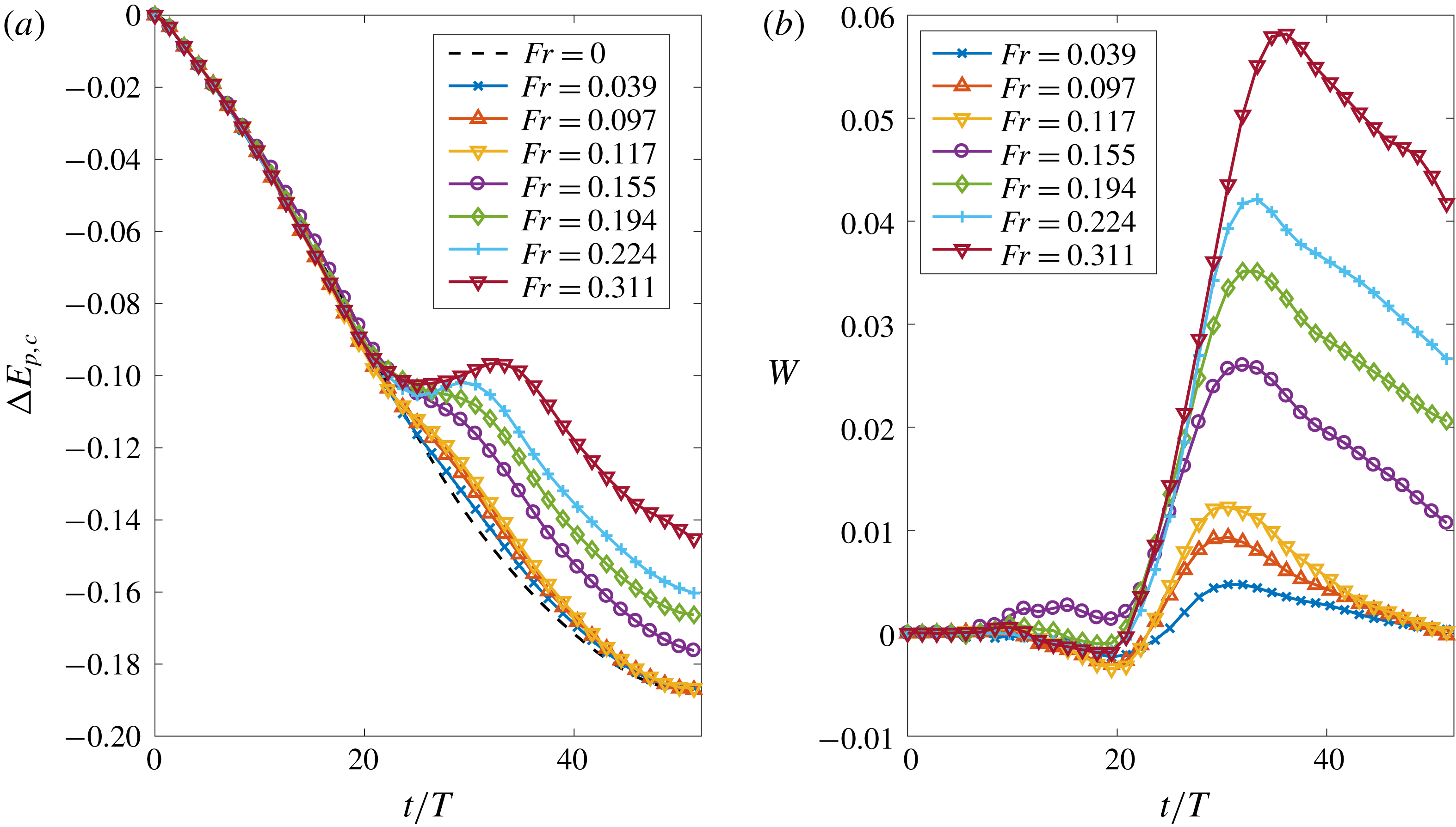
 $$\begin{eqnarray}\displaystyle W(t)=\unicode[STIX]{x0394}E_{p,c}(t)-(\unicode[STIX]{x0394}E_{p,c}(t))_{nw}, & & \displaystyle\end{eqnarray}$$
where the subscript
 $nw$
refers to the flow without a wave. Figure 9(a) shows the change in the gravity current potential energy
 $\unicode[STIX]{x0394}E_{p,c}(t)$
as a function of time, for various wave heights. For
 $Fr<0.155$
the influence of the wave is temporary and weak, so that soon the current energy again approaches its value without a wave. A clear regime change is observed for
 $Fr\geqslant 0.155$
, where the wave is seen to have a longer-lasting effect on the potential energy of the current fluid. This is confirmed by the amount of work
 $W$
displayed in figure 9(b), which demonstrates that small wave heights lead to a rapid and full recovery in the sense that soon again
 $W\rightarrow 0$
. This suggests that small waves do not increase the amount of irreversible mixing during the current–wave interaction, a hypothesis that will be examined in more detail below. For large wave Froude numbers
 $Fr\geqslant 0.155$
, on the other hand,
 $W$
reaches a much higher peak, and subsequently decreases only over a much longer time scale.
The above discussion of the energy budget indicates that for low wave Froude numbers, the wave temporarily slows down the current but does not increase the amount of mixing. Thus, the available potential energy is not reduced by the current–wave interaction, so that the current fluid can thus resume its release of potential energy upon the completion of this interaction. For large wave Froude numbers, on the other hand, the current is not only slowed down by the wave but it is also mixed, so that the potential energy available for subsequent release is reduced.
(a) Change in gravity current fluid potential energy as a function of time for various wave heights. (b) Work performed by the wave on the gravity current fluid as a function of time for various wave heights. Wave heights of
 $Fr\geqslant 0.155$
are seen to have a lasting effect on the potential energy budget of the gravity current fluid.

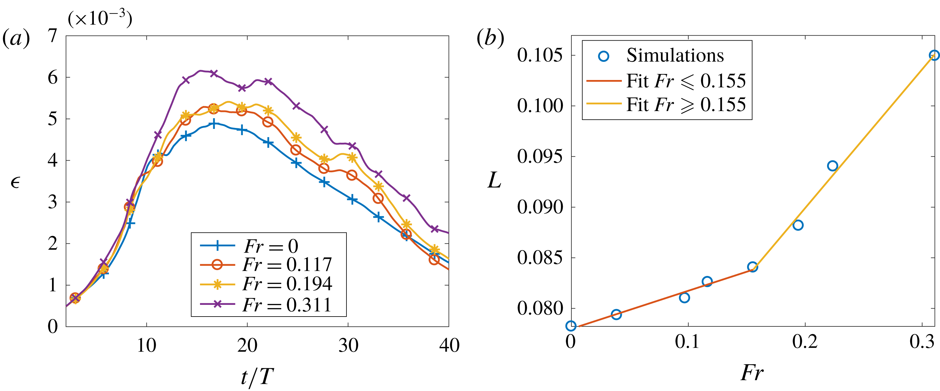
Figure 10(a) shows the volume integral
 $\unicode[STIX]{x1D716}(t)$
of the dissipation rate as a function of time for various
 $Fr$
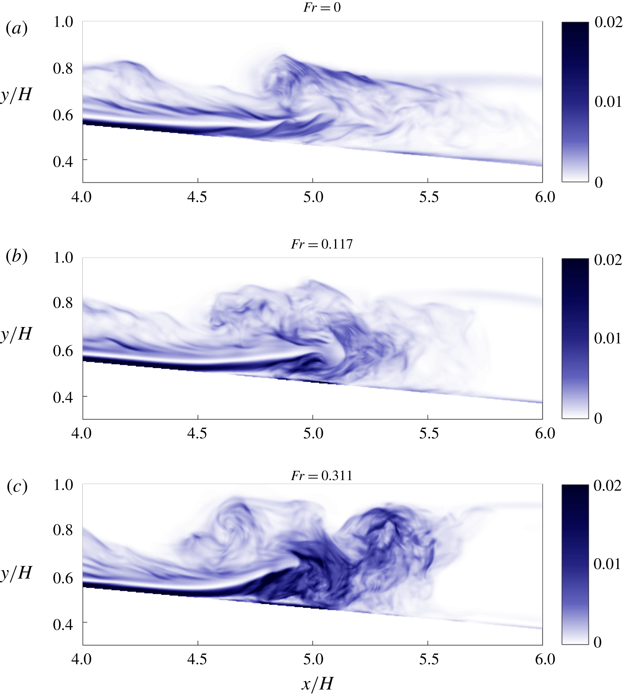
values. During the initial phase, dissipative processes in the bottom boundary layer of the current dominate (figure 11), while contributions from the wave propagating along the pycnocline are relatively minor. Hence,
 $\unicode[STIX]{x1D716}(t)$
is nearly independent of the wave height. Once the current and the wave begin to interact at
 $t/T\geqslant 10$
, however, dissipative effects within the larger region associated with the decapitation of the raised head gain importance, and
 $\unicode[STIX]{x1D716}(t)$
increases strongly with
 $Fr$
. This is reflected by the cumulative losses
 $L$
at the final simulation time (cf. figure 10
b). The slope
 $\text{d}(L)/\text{d}(Fr)$
becomes significantly steeper above
 $Fr\approx 0.155$
, which confirms that the current–wave interaction dominates the dissipation rate in this regime. The qualitative and quantitative evidence of a phenomenological change in the current–wave interaction motivates us to define a transitional Froude number, whose precise value depends on the experimental parameters and cannot, therefore, be readily generalized to other set-ups. For
 $Fr$
above
 $0.155$
the current–wave interaction is the dominant source of viscous dissipation and for
 $Fr$
below this value dissipation in the bottom boundary layer of the gravity current is dominant.
(a) Volume integral of the viscous dissipation
 $\unicode[STIX]{x1D716}$
as a function of time for various wave Froude numbers. (b) Cumulative viscous losses as a function of the wave Froude number. The slope of the cumulative viscous losses versus wave height increases above
 $Fr\approx 0.155$
.

Spanwise-averaged instantaneous viscous dissipation
 $\langle (2/Re)\unicode[STIX]{x1D634}_{ij}\unicode[STIX]{x1D634}_{ij}\rangle _{z}(x,y,t)$
at
 $t/T=26$
in the absence of a wave (a), in the presence of a wave at
 $Fr<0.155$
(b) and in the presence of a wave at
 $Fr>0.155$
(c). The wave (
 $Fr=0.117$
) slows down the current and somewhat increases the dissipation in the vicinity of the head and close to the slope. On the other hand, the wave at
 $Fr=0.311$
leads to strong dissipation away from the slope, within the uplifted current front.

3.5 Wave-induced irreversible mixing
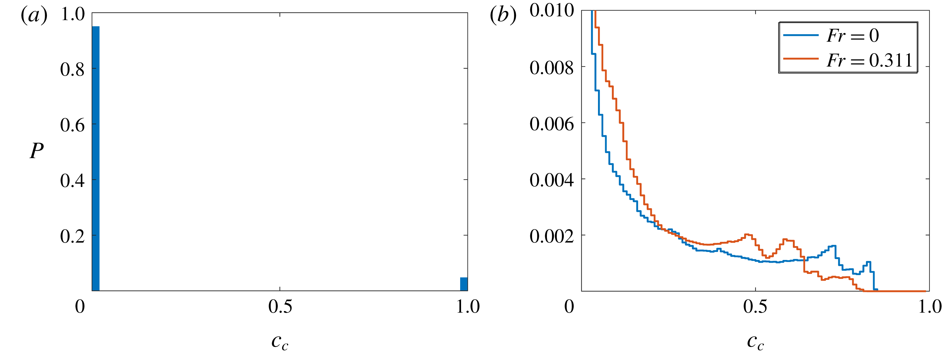
We proceed to analyse how the current–wave interaction affects the mixing of the gravity current fluid with the ambient, and specifically the amount of irreversible mixing that it triggers. Towards that end, we calculate the discrete probability density function (p.d.f.), or histogram, of the current fluid concentration
 $c_{c}(t)$
. We divide the concentration range
 $[0,1]$
into
 $N=400$
equally spaced bins, and count the number of grid cells within each bin. By normalizing with the total number of cells in the entire computational domain, we obtain the relative occurrence
 $P_{i}(t),~i=0,N-1$
of grid cells whose concentration
 $c$
falls within the range
 $i/N<c_{c}(\boldsymbol{x},t)<(i+1)/N$
, with
 $\sum _{i=0}^{N-1}P_{i}(t)=1$
. Initially, the concentration is either
 $c_{c}=0$
(outside the lock) or
 $c_{c}=1$
(inside the lock), so that
 $P_{i}(0)=0$
for
 $i=[1,N-2]$
,
 $P_{N-1}(0)=V_{1}/V_{tot}$
and
 $P_{0}(0)=(V_{tot}-V_{1})/V_{tot}$
(cf. figure 12
a). As the current moves down the slope and mixes with the ambient, regions of intermediate concentrations form via stirring and mixing.
(a) Initial histogram of gravity current fluid concentration
 $c_{c}$
. The discrete p.d.f.
 $P$
is the same for all Froude numbers and only depends on the ratio of lock volume to total volume. (b) The p.d.f. of gravity current fluid concentration
 $c_{c}$
at
 $t/T=52.14$
. The discrete p.d.f.
 $P$
(staircase plot for readability) shows an increase in intermediate concentrations for
 $Fr=0.311$
compared to the no-wave case (
 $Fr=0$
). Note that the vertical axis is clipped to
 $Pr=0.01$
for readability, as most of the ambient remains unmixed.

Figure 12(b) shows the final histograms at
 $t/T=52.14$
in the absence of a wave, as well as for the largest wave height
 $Fr=0.311$
. By this time, both flows have succeeded in diluting the gravity current fluid, so that values
 $c_{c}>0.85$
are no longer found. Closer inspection reveals that the
 $Fr=0.311$
wave has shifted both tails of the histogram more strongly towards the centre, as compared to the case without a wave. The background potential energy can now be calculated as a function of time and wave height in order to quantify the irreversible mixing observed in the histograms.
The background potential energy of a variable-density flow field corresponds to the lowest amount of potential energy that the system can achieve by an optimal redistribution of the fluid elements so that the fluid density decreases with height (Winters et al.
Reference Winters, Lombard, Riley and D’Asaro1995). In a closed system, it can only increase with time and its increase is a direct measure of irreversible mixing. The background potential energy is calculated from the sorted salinity profile written as
 $s(y^{\ast })$
, where
 $y^{\ast }$
maps the vertical coordinate of each fluid parcel to its sorted location. Profile
 $s(y^{\ast })$
is calculated directly from the histograms of concentration for
 $c_{c}$
and
 $c_{w}$
and we refer the reader to Winters et al. (Reference Winters, Lombard, Riley and D’Asaro1995) for the details of its calculation. Note that because of the slopping bottom, the calculation of the sorted profile is slightly more involved and results in a modified expression for the background potential energy given by
 $$\begin{eqnarray}\displaystyle E_{b}(t)=\int _{0}^{y_{N}^{\ast }}s(y^{\ast })A(y^{\ast })y^{\ast }\,\text{d}y^{\ast }, & & \displaystyle\end{eqnarray}$$
where
 $A(y^{\ast })$
is the horizontal area of the fluid domain at height
 $y^{\ast }$
.
For all simulations, the rate of change of background potential energy was found to reach a maximum during the initial interaction between the current and the pycnocline, i.e. for
 $t_{1}\leqslant t\leqslant t_{2}$
with
 $t_{1}/T\approx 10$
and
 $t_{2}/T\approx 30$
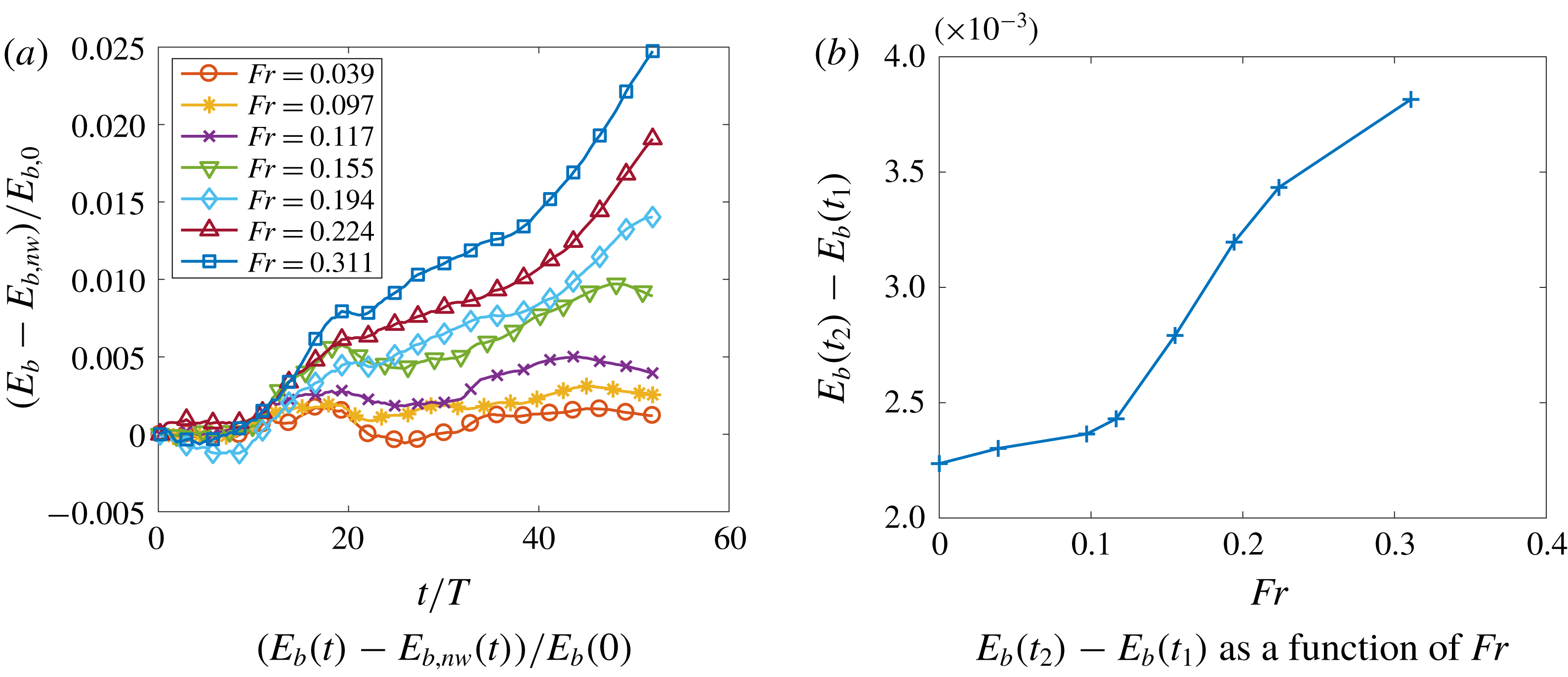
. The difference of background potential energy with and without a wave, normalized by the initial background potential energy, is plotted in figure 13(a) as a function of time for several wave Froude numbers
 $Fr$
. Note that
 $E_{b}(t=0)$
is the same for all
 $Fr$
. As expected, the presence of a wave leads to a considerable increase in irreversible mixing, which depends directly on the wave height.
Wave-induced mixing is most effective for a shorter period of time (
 $t_{1}\leqslant t/T\leqslant t_{3}$
, where
 $t_{3}\approx 20$
) than the peak production period. Irreversible mixing produced during the wave–current interaction is measured as the difference between background potential energy before and after interaction, i.e.
 $E_{b}(t_{2})-E_{b}(t_{1})$
. This is plotted in figure 13(b), and reveals once again the change in behaviour of the flow at higher wave Froude numbers. The background potential energy produced during the interaction increases monotonically with wave height but does so much more distinctively for
 $Fr\geqslant 0.155$
. We also note that the amount of background potential energy produced during this time interval for the largest wave is close to twice that of the case in the absence of a wave. It is also interesting to note in figure 13(a) that the three largest waves lead to a secondary increase in irreversible mixing at late times, i.e.
 $t/T\geqslant 40$
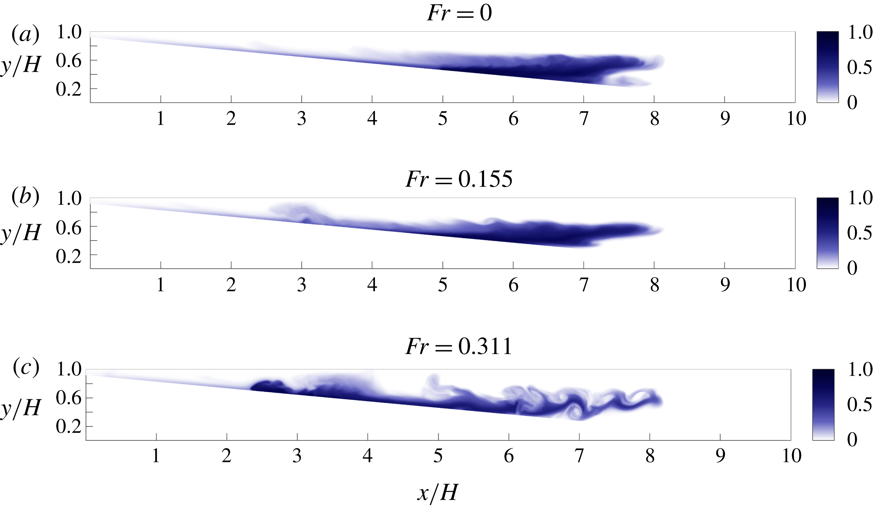
. Indeed, when the reflected component of the gravity current forms an upslope current, irreversible mixing increases through entrainment (figure 14). Additionally, vertically transported gravity current fluid is found in higher concentrations above the slope for cases with waves at
 $Fr>0.155$
. This fluid was transported during the decapitation process and is thus able to mix efficiently with ambient fluid post-interaction, contributing to enhanced mixing at later times. Finally, Kelvin–Helmoltz-like structures, or numerical mimics thereof, are seen to perturb the intrusion at late times and for large waves. The size of the structures and their two-dimensional nature suggest that they contribute only little to mixing, but their existence is more likely due to the strength of the wave reflection on the right-hand wall and is thus limited to a laboratory setting.
(a) Difference in background potential energy with respect to the case without a wave (nw) as a function of time for various wave Froude numbers. (b) Background potential energy produced between
 $t_{1}/T=10$
and
 $t_{2}/T=30$
, corresponding to the time interval of strong background potential energy production, plotted as a function of the wave Froude number.

Snapshot of the depth-averaged gravity current fluid concentration at
 $t/T=52.14$
for three wave Froude numbers. Mixing is induced by entrainment in the reflected, upslope-propagating component of the gravity current. Interactions between the intrusion and the wave reflected off the right-hand wall lead to additional mixing that is not directly linked to the current–wave interaction.

3.6 Influence of density ratio
An essential aspect of the wave–current interaction was left unexplored in the experiments of Hogg et al. (Reference Hogg, Egan, Ouellette and Koseff2018), where the density ratio
 $(\unicode[STIX]{x1D70C}_{2}-\unicode[STIX]{x1D70C}_{0})/(\unicode[STIX]{x1D70C}_{1}-\unicode[STIX]{x1D70C}_{0})=c_{2}/c_{1}$
was held constant at 0.8. Section 3.4 demonstrated the importance of the energy transfer between the wave and the current, which should be a strong function of their respective excess densities. In order to investigate this aspect, we conduct a series of simulations for a constant wave Froude number
 $Fr=0.194$
and density ratios
 $c_{2}/c_{1}=0.6$
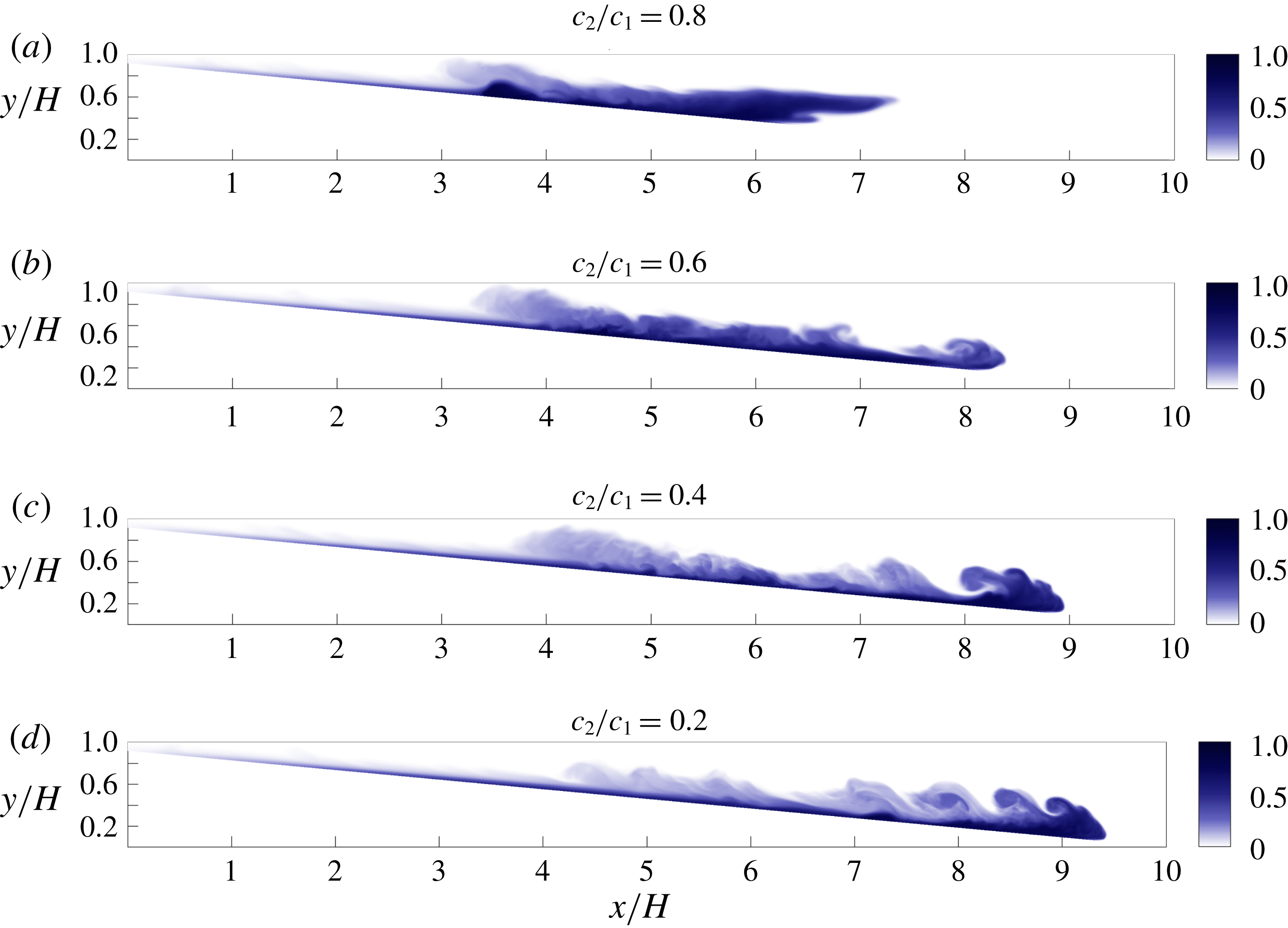
, 0.4 and 0.2. Snapshots of the corresponding spanwise-averaged gravity current fluid concentration at
 $t/T=43.45$
are shown in figure 15. The original density ratio of
 $c_{2}/c_{1}=0.8$
leads to a complete modification of the flow in the presence of the wave, as previously described. The hyperpycnal component of the current is strongly delayed and depleted post-interaction and a strong upslope current is formed. At
 $c_{2}/c_{1}=0.6$
, the head of the current is altered but persists and continues to move downslope. There is no sign of an intrusion, but the body of the current appears to be diluted on a large volume above the slope. A thin layer of gravity current fluid separates the head from the diluted body, which suggests that the wave failed to decapitate the current but strongly altered the propagation of the body of the current. At
 $c_{2}/c_{1}=0.4$
, most of the head of the current retained its shape and the diluted body of the current was able to stay close to the head of the current after penetration of the pycnocline. At
 $c_{2}/c_{1}=0.2$
, the gravity current completely recovers its natural dynamics with a strong head followed directly by an entrainment region forming the body of the current. As in § 3.2, the mass flux across an interrogation plane located at
 $x_{b}/H=7$
is averaged over time and plotted as a function of
 $y$
(figure 16
a). The mass flux substantially increases as
 $c_{2}/c_{1}$
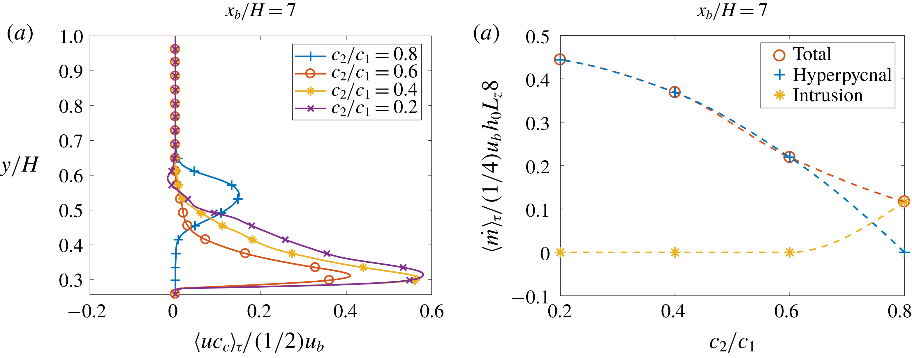
decreases, and transfers from an almost purely intrusive component for the largest density ratio to a purely hyperpycnal component for all other ratios. The result at
 $c_{2}/c_{1}=0.6$
is particularly interesting as the mass flux is overall strongly reduced compared to the two smaller ratios, yet no component of the flow is part of a rightward-propagating intrusion. This could indicate that the wave has had the effect of stopping the propagation of partially diluted gravity current fluid as an intrusion, yet allowed the propagation of the hyperpycnal component. Figure 16(b) illustrates the decline in total mass flux with the increase of the density ratio and stresses the idea of a transition for
 $0.6<c_{2}/c_{1}<0.8$
to a purely intrusive flow. Predictability of current dilution and correspondingly of entrainment is paramount to determine the exact transition point from a purely hyperpycnal to a purely intrusive flow as a function of the density ratio. The coupling of wave-induced transport with this transition is beyond the scope of the project. This nonetheless presents a new opportunity for experimental and modelling work on the effect of waves on intrusions in a strongly hyperpycnal flow (say
 $c_{2}/c_{1}<0.6$
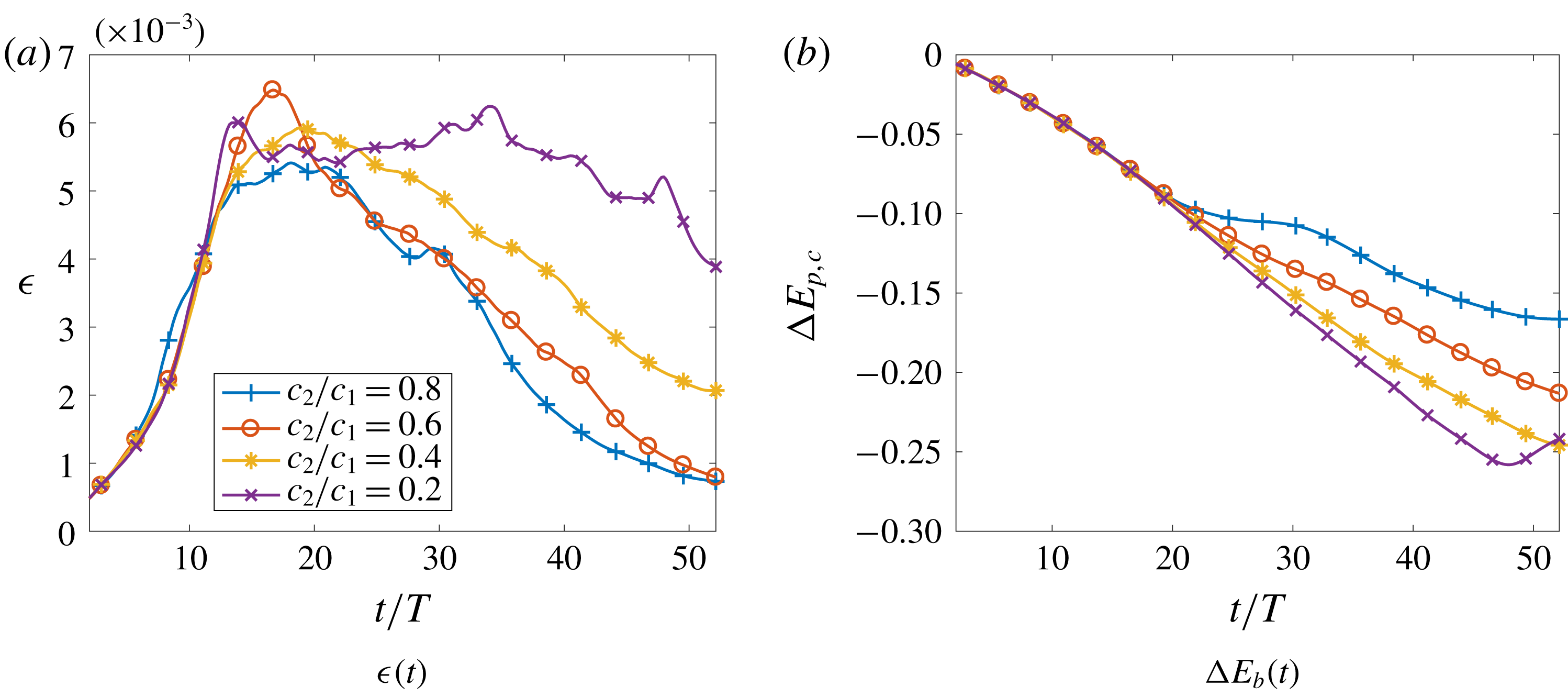
in this particular scenario). An analysis of viscous dissipation (figure 17
a) reveals an increase in dissipation as
 $c_{2}/c_{1}$
decreases. Indeed, less kinetic energy is conceded by the current to raise the pycnocline of the dense lower ambient, thus allowing for viscous dissipation to act on longer times as the current propagates. The change in potential energy associated with the gravity current fluid is plotted in figure 17(b). Momentum carried by the wave decreases as
 $c_{2}/c_{1}$
decreases and thus less energy is converted back into current potential energy during the interaction. At
 $c_{2}/c_{1}=0.2$
, the rate of conversion of potential energy into kinetic energy and dissipation losses is almost constant over the propagation time. The increase at the later time simply indicates that the current has reached the right-hand wall and is thus pushed upwards. We further quantify the effect of the concentration ratio by isolating the gravity current fluid present in the upper region of the domain, defined by
 $y\geqslant h_{l}$
, where
 $h_{l}$
defines the initial location of the lower pycnocline of the ambient fluid. Isolating this component for a given wave height but various ratios
 $c_{2}/c_{1}$
allows us to directly measure the effect of the wave on vertical transport of gravity current fluid. We define the mass of gravity current fluid in the upper layer as
 $$\begin{eqnarray}\displaystyle m^{\ast }=\int _{\unicode[STIX]{x1D6FA}}^{\ast }c_{c}\,\text{d}V, & & \displaystyle\end{eqnarray}$$
Snapshot of the spanwise-averaged gravity current fluid concentration at
 $t/T=43.45$
for
 $Fr=0.194$
and four density ratios
 $c_{2}/c_{1}$
.

where
 $\unicode[STIX]{x1D6FA}^{\ast }=\unicode[STIX]{x1D6FA}(y\geqslant h_{l})$
and
 $\unicode[STIX]{x1D6FA}$
represents the total fluid volume. Mass
 $m^{\ast }$
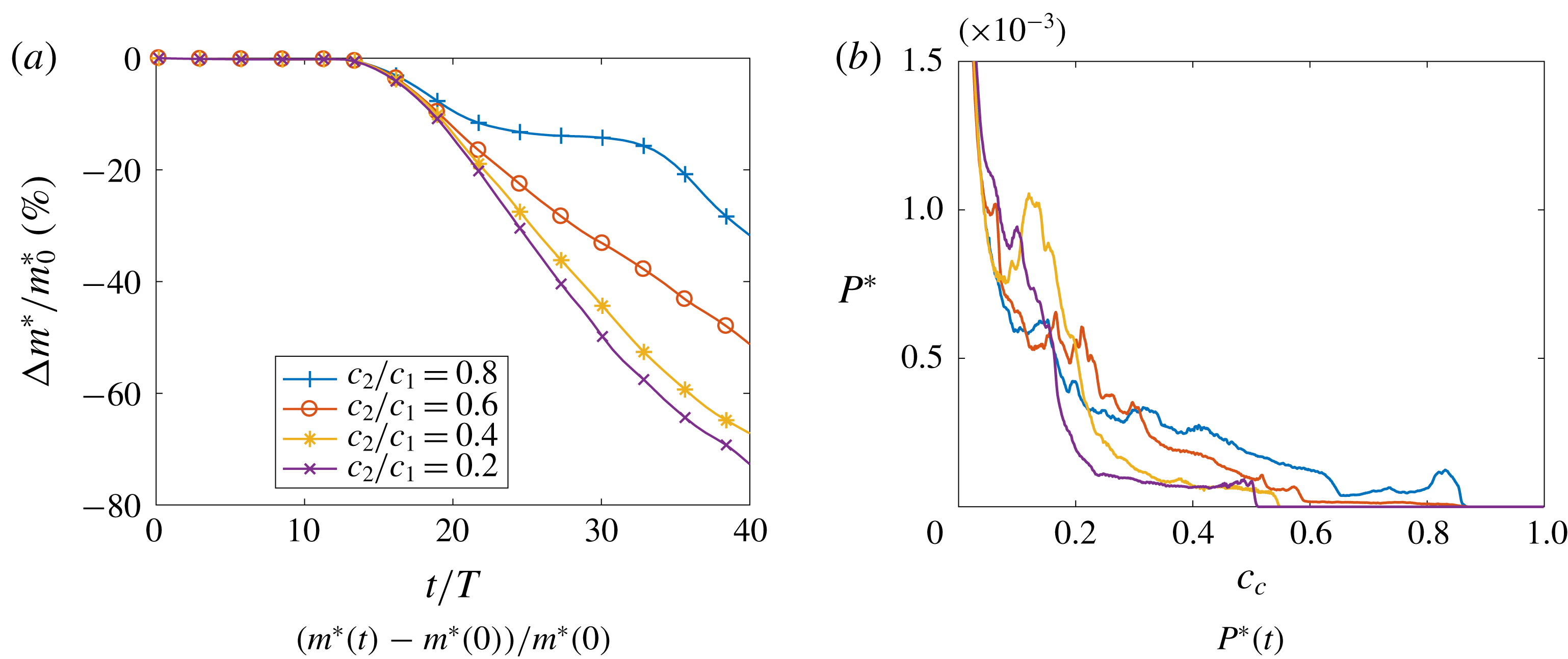
is plotted in figure 18(a) and directly explains the change in potential energy observed in figure 17(b). Gravity current fluid upon interaction with a dense wave remains in larger amount above the pycnocline and mixes ambient fluid, while gravity current fluid interacting with a lighter wave penetrates the pycnocline, reducing vertical transport of dense gravity current fluid. During the decapitation process and up to a time of
 $t/T=30$
after release, less than
 $20\,\%$
of the gravity current fluid is able to penetrate the lower pycnocline for the maximum ratio of
 $c_{2}/c_{1}=0.8$
. In comparison, the smallest ratio of
 $c_{2}/c_{1}=0.2$
leads to
 $60\,\%$
of the gravity fluid penetrating through the pycnocline by the same instant in time. While smaller ratios lead to more dissipation (figure 17
a) due to the ability of the current to release its potential energy (figure 17
b), it is expected that higher concentration ratios will lead to more mixing of gravity current fluid in the upper layer and thus away from the slope. This is shown by calculating the p.d.f.
 $P^{\ast }(t)$
of gravity current fluid concentration
 $c_{c}$
in the upper domain
 $\unicode[STIX]{x1D6FA}^{\ast }$
. Intermediate concentrations are present in the upper region for the largest ratio
 $c_{2}/c_{1}$
. This is due to the vertical transport of partially mixed fluid during the decapitation process. Naturally, only concentrations below
 $c_{2}$
are present in the upper domain for all simulations. This is due to the fact that any larger concentration of gravity current fluid is denser than the lower ambient fluid and can thus penetrate the pycnocline. This results in far fewer cells of intermediate concentration of gravity current fluid for lower values of
 $c_{2}/c_{1}$
.
(a) Time-averaged profile of the horizontal flux of gravity current fluid
 $uc_{c}$
as a function of
 $y$
. (b) Discrete contributions of the hyperpycnal and intrusive gravity current to the total time-averaged mass flux as a function of the density ratio, for
 $Fr=0.194$
. The averaging window is
 $t/T\in [26.07,52.14]$
, i.e from the beginning of the intrusion to the end of the numerical simulation.

Wave Froude number
 $Fr=0.194$
. (a) Viscous dissipation as a function of time for various initial concentration ratios
 $c_{2}/c_{1}$
between the bottom ambient fluid and the gravity current fluid. (b) Change in potential energy of the gravity current fluid as a function of time for various initial concentration ratios
 $c_{2}/c_{1}$
.

Wave Froude number
 $Fr=0.194$
. (a) Relative change in mass of gravity current fluid present above the initial pycnocline defined by
 $y=h_{l}$
as a function of time for various initial concentration ratios
 $c_{2}/c_{1}$
between the bottom ambient fluid and the gravity current fluid. (b) The p.d.f. of the gravity current fluid concentration above the initial pycnocline
 $y=h_{l}$
for various initial concentration ratios
 $c_{2}/c_{1}$
at
 $t/T=43.45$
.

4 Summary
Experiments by Hogg et al. (Reference Hogg, Egan, Ouellette and Koseff2018) of a downslope gravity current interacting with an internal wave travelling at the pycnocline of a two-layer stratification were reproduced using direct numerical simulations. The simulation parameters are at scale with the experiments in terms of the Reynolds number, density ratio and wave Froude number, or wave height. The numerical simulations corroborate the experimental observations of a strong current–wave interaction for sufficiently large waves, referred to by Hogg et al. (Reference Hogg, Egan, Ouellette and Koseff2018) as the current head decapitation. The numerical simulations also corroborate observations of a reduced mass flux of the gravity current as it penetrates the pycnocline compared to a similar stratification in the absence of a wave. The mass flux is dominated by the intrusion of partially mixed gravity current fluid along the pycnocline, at its height of neutral buoyancy. Both the intrusion and hyperpycnal components of the gravity current mass flux downslope from the point where the pycnocline meets the slope are reduced in the presence of the wave. The overall mass-flux reduction for the largest tested wave height is of the order of
 $50\,\%$
, which agrees well with the results of Hogg et al. (Reference Hogg, Egan, Ouellette and Koseff2018). Close inspection of the flow dynamics during interaction with the wave reveals how the decapitation process occurs: momentum transferred by the wave into the gravity current leads to a reverse flow that separates from the head of the current and propagates back upslope. Fluid from the head is simultaneously split into a hyperpycnal component and a vertically transported component that lifts into the ambient. Part of this vertically transported – or decapitated – gravity current fluid then gets transported to the left by the reverse current occurring at the top of the domain and transported to the right as an intrusion at the pycnocline. This dynamical process translates in a change in the front velocity of the current. Individual measurements of the hyperpycnal and intrusion components of the gravity current in terms of front location reveal that both fronts are slowed down during interaction as wave height is increased. However, a change in behaviour is observed for
 $Fr\geqslant 0.155$
: while the front location of the intrusion is not strongly affected, the front of the hyperpycnal current comes to a complete stop and only resumes its progression after interaction with the wave. This observation translates the vertical transport of the decapitated head of the current, and the formation of a new hyperpycnal front from the body of the current that then resumes its along-slope propagation.
The existence of a transitional Froude number above which the decapitation process can occur has direct consequences for the energy budget of the flow. In the absence of a wave, kinetic energy is generated by the release of potential energy contained in the gravity current. As it reaches the pycnocline, the gravity current loses kinetic energy to raise the potential energy of the dense lower ambient fluid. In the presence of a wave, both the gravity current fluid and the lower ambient fluid release potential energy into kinetic energy. Upon interaction, the kinetic energy drops markedly to the benefit of the potential energy of both the lower ambient and gravity current fluids. Small waves lead to no persistent change of the gravity current potential energy whereas large waves seem to irreversibly transfer kinetic energy into gravity current potential energy. This regime change of potential energy transfers in the gravity current fluid again occurs for
 $Fr\approx 0.155$
. Viscous dissipation reaches a maximum during the current–wave interaction and increases with wave height. Viscous losses increase more rapidly with wave height past the transitional value of the Froude number, due to stronger stirring in the vertically transported head of the current.
Time-resolved quantification of irreversible mixing is achieved through calculation of the global background potential energy of the salinity field. The effect of the wave on production of background potential energy, or equivalently on destruction of available potential energy, is most strongly felt during the initial wave–current interaction. Large waves lead to continuously more irreversible mixing than in the absence of a wave, while smaller waves lead to a more transient yet comparable production of background potential energy than in the absence of a wave. Production of background potential energy during the wave–current interaction goes through the same regime change as the global energy budget when the removal of the head by the wave occurs. In the decapitation regime, background potential energy change increases rapidly with wave height and reaches close to double that of the no-wave case for
 $Fr=0.311$
.
The effect of the density ratio
 $(\unicode[STIX]{x1D70C}_{2}-\unicode[STIX]{x1D70C}_{0})/(\unicode[STIX]{x1D70C}_{1}-\unicode[STIX]{x1D70C}_{0})=c_{2}/c_{1}$
was finally explored as it is expected to play a great role in the change in energy transfers at large wave heights. A wave Froude number of
 $Fr=0.194$
is chosen and the concentration ratio was successively decreased. In the presence of a wave, the decrease in density ratio quickly leads to a marked change in the behaviour of the gravity current mass flux below the pycnocline. Below a transitional value, the mass flux is solely due to a hyperpycnal component and no intrusion of partially mixed fluid is observed to propagate to the right. Above the transitional value, all the flux is in the intrusion. The behaviour at the largest density ratio that still leads to no intrusion is particularly interesting, as it appears that the wave served to retain partially mixed fluid close to the point of interaction instead of this mixed fluid forming an intrusion. In addition, smaller ratios allow the gravity current to release more potential energy after reaching the pycnocline, yielding increased dissipation below the pycnocline. The effect of the wave on changes in current fluid potential energy becomes negligible at lower density ratios and it is expected that values of
 $c_{2}/c_{1}$
close to unity are necessary to observe the removal of the head of the current by the wave. While smaller ratios appear to be favourable to mixing due to the generation of additional kinetic energy during the propagation of the current, mass retention and mixing above the pycnocline is strongly reduced. Regions of intermediate concentrations formed during the decapitation process are absent at lower ratios, and only fluid of concentration below the lower ambient value is able to stay above the pycnocline. In natural settings, regions of strongly layered stratification close to shores are thus far better candidates for the observation of such high-intensity events as the removal of the head by an internal wave than regions where the current is much denser than both layers. Alternatively, strong coupling events can be avoided, or intentionally generated, by adjusting the density ratio of the dense ambient to the released current.
Acknowledgements
The authors wish to thank C. Hogg for his contributions during the early stages of the investigation. The authors would also like to express their appreciation to the referees for their feedback and suggestions. E.M. gratefully acknowledges the support and hospitality he received as Shimizu Visiting Professor at Stanford University. Funding for this work was provided under NSF grants CBET-1067847 (E.M.) and OCE-1634389 (N.T.O. and J.R.K.). Computational resources for this work used the Extreme Science and Engineering Discovery Environment (XSEDE), which was supported by the National Science Foundation, USA, grant no. TG-CTS150053.