1. Introduction
In the core region of tokamaks, gradients of plasma parameters drive turbulence at microscales of the order of the ion or electron gyroradius. The resulting losses of particles, momentum and heat towards the vessel wall set a limit for the densities and temperatures that can be sustained in the device, which in turn limits the rate of fusion reactions. In current and future experiments such as JET and ITER, the core plasma is, in part, heated and fuelled by injecting energetic beams of neutral atoms of hydrogen isotopes (deuterium and tritium). As the beams penetrate into the core, they apply a torque on the plasma and make it spin toroidally. Experimental, theoretical and computational results have shown that the presence of shear in the toroidal rotation can substantially affect turbulent transport: shear in the flow perpendicular to the mean magnetic field has been found to reduce transport, while a gradient in the parallel flow can enhance transport, see e.g. Catto, Rosenbluth & Liu (Reference Catto, Rosenbluth and Liu1973), Artun & Tang (Reference Artun and Tang1992), Barnes et al. (Reference Barnes, Parra, Highcock, Schekochihin, Cowley and Roach2011a), Casson et al. (Reference Casson, Peeters, Camenen, Hornsby, Snodin, Strintzi and Szepesi2009), Dimits et al. (Reference Dimits, Williams, Byers and Cohen1996), Mantica et al. (Reference Mantica, Strintzi, Tala, Giroud, Johnson, Leggate, Lerche, Loarer, Peeters and Salmi2009), McKee et al. (Reference McKee, Gohil, Schlossberg, Boedo, Burrell, de Grassie, Groebner, Moyer, Petty and Rhodes2009), Peeters & Angioni (Reference Peeters and Angioni2005), Synakowski et al. (Reference Synakowski, Batha, Beer, Bell, Bell, Budny, Bush, Efthimion, Hammett and Hahm1997), Waelbroeck & Chen (Reference Waelbroeck and Chen1991), Waltz, Dewar & Garbet (Reference Waltz, Dewar and Garbet1998), Waltz et al. (Reference Waltz, Kerbel, Milovich and Hammett1995) and Waltz et al. (Reference Waltz, Staebler, Candy and Hinton2007).
The first implementation of flow shear for local, $\delta f$ gyrokinetic simulations was developed by Hammett et al. (Reference Hammett, Dorland, Loureiro and Tatsuno2006) in the linearly implicit-in-time code GS2 (Kotschenreuther, Rewoldt & Tang Reference Kotschenreuther, Rewoldt and Tang1995), and was later applied to others including GENE (Jenko et al. Reference Jenko, Dorland, Kotschenreuther and Rogers2000), GKW (Peeters et al. Reference Peeters, Camenen, Casson, Hornsby, Snodin, Strintzi and Szepesi2009) and CGYRO (Candy & Belli Reference Candy and Belli2018). In this approach, the system of gyrokinetic and Maxwell equations is expressed in the frame that rotates and shears along with the flow, allowing the equations to be Fourier analysed across the mean magnetic field. The effective radial wavenumber in the laboratory frame – a constant without flow shear – becomes time-dependent in the presence of flow shear. To retain the benefits of using a code that is implicit in time, this approach to flow shear approximates such time-dependences by combining a nearest point approximation on a fixed grid, together with a wavenumber remapping method. This ensures that the computationally expensive part of the implicit scheme only needs to be executed at initialisation, rather than at every time step. However, many experiments only sustain modest levels of flow shear, for which the radial wavenumber evolves very slowly: simulations then produce long periods of time where the perpendicular flow shear has no effect, separated by discrete jumps in wavenumber. We wish to avoid this unphysical behaviour, and consider here an improved, continuous-in-time approach to flow shear.
This work is organised as follows. First, we give a brief overview in § 2 of the gyrokinetic ordering, the coordinates that are used, and the system of Fourier-analysed equations that have to be solved. In the next section, we summarise the main algorithm of GS2, as well as the discrete-in-time approach to flow shear developed by Hammett et al. Following this, we present a new algorithm that treats flow shear continuously over time. Finally, in § 4, we show numerical results obtained with GS2 that test the implementation of the continuous-in-time approach, and compare it with the discrete-in-time method.
2. Model
In this section, we give a brief overview of the standard orderings assumed in $\delta f$ gyrokinetic flux tube codes such as GS2 and present the equations solved in the code. We then explain how the presence of a sheared background toroidal flow modifies the spectral representation that is used in the plane perpendicular to the magnetic field.
2.1. Orderings and equations
The $\delta f$ gyrokinetic description (Catto Reference Catto1978; Frieman & Chen Reference Frieman and Chen1982) hinges on scale separations in both time and space: the fluctuations of interest are chosen to be much slower than the gyromotion of particles around magnetic field lines, and the gyroradii are assumed to be much smaller than the equilibrium length scale. The distribution function $f$
 can be described as the sum of an equilibrium piece $\langle \,f \rangle$
 and a fluctuating piece $\delta f = f-\langle \,f \rangle$
 , where $\langle \cdot \rangle$
 denotes an ensemble average. The fluctuating part is ordered to be much smaller than the equilibrium quantity,

where $\rho = \vert \boldsymbol {\rho }\vert = \vert \hat {\boldsymbol {b}}\times \boldsymbol {v}/\varOmega \vert$ is the gyroradius and $L$
 is the equilibrium length scale (typically the minor radius of the tokamak). Here $\hat {\boldsymbol {b}}=\boldsymbol {B}/B$
 denotes the unit vector in the direction of the magnetic field $\boldsymbol {B}$
 , $B$
 is the norm of $\boldsymbol {B}$
 , $\boldsymbol {v}$
 is the velocity of the particle and $\varOmega =eZ B/mc$
 is the gyrofrequency with $Z$
 the charge number of the particle, $e$
 the elementary charge, $m$
 the particle mass and $c$
 the speed of light. In the frame moving with the background plasma flow $\boldsymbol {u}$
 , the fluctuations described by $\delta f$
 are associated with a typical frequency $\omega \sim \rho _*\varOmega$
 (Sugama & Horton Reference Sugama and Horton1998). The fluctuations are assumed to be elongated along field lines ($\sim L$
 ) but much thinner across field lines ($\sim \rho$
 ). On the other hand, the equilibrium part evolves on the energy confinement time scale $\tau _E\sim (\rho _*^2\omega )^{-1}$
 and has a typical length scale of order $L$
 both along and across field lines. To summarise the orderings are


Within this asymptotic expansion in $\rho _*$ , we restrict ourselves to the high-flow regime, in which the background flow $u$
 is first ordered to be comparable to the ion thermal speed $v_{\text {th},i}=\sqrt {2T_i/m_i}$
 , with $T_i$
 the ion temperature. We then consider a subsidiary expansion in the Mach number $M\equiv u/v_{\text {th},i}$
 such that $\rho _*\ll M \ll 1$
 , and we neglect second-order effects in $M$
 . In the high-flow regime, the background plasma flow is toroidal to lowest order in $\rho _*$
 , and the associated angular frequency $\varOmega _\phi$
 is constant on a magnetic flux surface (Catto, Bernstein & Tessarotto Reference Catto, Bernstein and Tessarotto1987): $\boldsymbol {u}=\varOmega _\phi (\psi ) R^2 \boldsymbol {\nabla }\phi + O({\rho _* v_{\text {th},i}})$
 with $\psi$
 the flux surface label, $R$
 the major radius and $\phi$
 the toroidal angle.
Making use of the assumptions above, one can express the Vlasov equation order by order in $\rho _*^n \varOmega f$ for $n=0,1,2$
 and average over the rapid gyromotion to obtain the gyrokinetic equation governing the evolution of fluctuations of the distribution function,

Here, the subscript $s$ labels the species, $\langle {\cdot } \rangle _{\boldsymbol {R}_s}=(2{\rm \pi} )^{-1}\int _0^{2{\rm \pi} } (\cdot )\,\textrm {d} \gamma$
 denotes an average over the gyrophase $\gamma$
 at fixed gyrocentre $\boldsymbol {R}_s=\boldsymbol {r}-\boldsymbol {\rho }_s$
 with $\boldsymbol {r}$
 the particle position, and derivatives are taken at fixed $(\boldsymbol {R}_s,\varepsilon _{s},\mu _{s})$
 , $g_s(\boldsymbol {R}_s,\varepsilon _{s},\mu _{s})=\langle \delta f_s \rangle _{\boldsymbol {R}_s}$
 is the gyroaveraged fluctuating distribution function, $\varepsilon _{s}=m_s w^2/2$
 is the particle kinetic energy, $\mu _{s}=m_s w_\perp ^2/2B$
 is the magnetic moment, $\varphi$
 is the fluctuating electrostatic potential, $\boldsymbol {w}=\boldsymbol {v}-\boldsymbol {u}$
 is the particle velocity relative to the background flow, $w_\parallel =\boldsymbol {w}\boldsymbol {\cdot } \hat {\boldsymbol {b}}$
 is its component along the magnetic field, ${I}(\psi )=R^2\boldsymbol {B}\boldsymbol {\cdot }\boldsymbol {\nabla }\phi$
 , and $F_{0,s}$
 is a Maxwellian distribution of velocities. The species-dependent guiding centre drift velocity $\boldsymbol {V}_{d,s}=\boldsymbol {V}_{B,s}+ \boldsymbol {V}_{C,s}$
 includes the $\boldsymbol {\nabla } B$
 and curvature drifts $\boldsymbol {V}_{B,s} = \hat {\boldsymbol {b}}/\varOmega _s\times [ w_\perp ^2\boldsymbol {\nabla }\ln (B)/2 + w_\parallel ^2 \hat {\boldsymbol {b}}\boldsymbol {\cdot }\boldsymbol {\nabla }\hat {\boldsymbol {b}}]$
 , as well as the Coriolis drift $\boldsymbol {V}_{C,s} = (2w_\parallel \varOmega _\phi /\varOmega _s)\hat {\boldsymbol {b}}\times (\hat {\boldsymbol {Z}}\times \hat {\boldsymbol {b}})$
 , with $\boldsymbol {w}_\perp = \boldsymbol {w}-w_\parallel \hat {\boldsymbol {b}}$
 the component of $\boldsymbol {w}$
 perpendicular to the magnetic field, and $\hat {\boldsymbol {Z}}$
 the unit vector in the vertical direction. The fluctuating $\boldsymbol {E}\times \boldsymbol {B}$
 drift is given by $\boldsymbol {V}_E = c\hat {\boldsymbol {b}}/B\times \boldsymbol {\nabla }\varphi$
 . For the purpose of this work, we are neglecting fluctuations of the magnetic field and the effects of collisions.
The system is closed with the quasineutrality equation,

where $n_s$ is the density of particles, and the brackets $\langle \cdot \rangle _{\boldsymbol {r}}$
 denote an average over the gyrophase at fixed particle position.
2.2. Shearing frame coordinates
Solving the gyrokinetic equation over a machine-sized domain can be computationally very expensive. Instead, GS2 and other ‘local’ codes focus on a thin, filament-like simulation domain known as a flux tube, which extends along a magnetic field line as it wraps around the torus. In directions perpendicular to $\boldsymbol {B}$ , the flux tube is assumed to be wide enough (several $\rho$
 ) for the fluctuations on one side of the domain to be decorrelated from the ones on the opposite side. Ideally the flux tube is kept much narrower than the equilibrium length scale $L$
 so that equilibrium quantities and their gradients can be considered as constant across $\boldsymbol {B}$
 in the simulation. Formally, it corresponds to the limit $\rho _*\rightarrow 0$
 . This local approximation ensures that fluctuations at either end of the perpendicular domain are not only decorrelated but also statistically identical. It is further assumed that two such instances of turbulence can be set exactly equal to one another without affecting the statistical properties of the simulation domain. Hence, periodic boundary conditions are enforced (Beer, Cowley & Hammett Reference Beer, Cowley and Hammett1995) perpendicular to $\boldsymbol {B}$
 .
In the local approximation, the toroidal angular frequency is given by $\varOmega _\phi (\psi )\simeq \Omega _{\phi ,0} + \Omega ^\prime _{\phi ,0} (\psi -\psi _0)$ , where the subscript $0$
 indicates that a quantity is evaluated along the central field line in the simulation domain and the prime denotes differentiation with respect to the flux label $\psi$
 . In the absence of flow shear ($\Omega ^\prime _{\phi ,0} = 0$
 ), GS2 works in the corotating frame $(\theta ,x,y)$
 , where the poloidal angle $\theta$
 serves as the coordinate parallel to the field, $x$
 is the radial coordinate and $y$
 is the coordinate perpendicular to the field line within the flux surface,


where $B_r$ is a reference magnetic field strength, $q(\psi )$
 is the safety factor, $r_\psi$
 is the half-diameter of a flux surface at the height of the magnetic axis, and $\alpha =\phi -q\vartheta -\Omega _{\phi ,0} t$
 is the field line label with

Note that the $x$ and $y$
 coordinates are not orthogonal.
In the presence of flow shear ($\Omega ^\prime _{\phi ,0}\neq 0$ ), the new terms appearing in the gyrokinetic equation through $\boldsymbol {u}\boldsymbol {\cdot }\boldsymbol {\nabla }$
 are not periodic in $x$
 and so the periodic solution obtained by Fourier transforming in $(x,y)$
 is not consistent with the equation. The solution adopted in GS2 (Hammett et al. Reference Hammett, Dorland, Loureiro and Tatsuno2006) is to restore periodicity by working in the shearing frame $(\theta ,x,y^*)$
 , with

where the shearing rate is defined as

From here on, the star superscript will be used to indicate that the associated quantity is time dependent in the presence of flow shear. It is not to be confused with the usual notation for complex conjugates.
2.3. Spectral representation
Given the periodic boundary conditions in the perpendicular directions discussed above, any fluctuating quantity $\varPhi$ can be expressed as a Fourier series in the shearing frame,

where we define the wavevector $\boldsymbol {k} = k_x\boldsymbol {\nabla } x + k_y\boldsymbol {\nabla }y^*$ , with wavenumbers given by $k_x = j_x \Delta k _x$
 , $k_y = j_y \Delta k_y$
 , grid spacings by $\Delta k _x=2{\rm \pi} /L_x$
 , $\Delta k_y=2{\rm \pi} /L_y$
 , $L_x$
 and $L_y$
 are the perpendicular sizes of the computational domain, and with the integer indices spanning $-(N_x-1)/2 \leq j_x \leq (N_x-1)/2$
 and $0\leq j_y < N_y$
 , respectively. Note that the exponent can also be written in terms of $(x,y)$
 as $\textrm {i}k^*_x(t)x+\textrm {i}k_yy$
 where $k^*_x(t)\equiv k_x- k_y\gamma _E t$
 is the effective, time-dependent radial wavenumber in the laboratory frame. With this spectral representation in the shearing frame, time dependences due to flow shear appear when either a gradient or a gyroaverage is applied to a fluctuating quantity,

with $\boldsymbol {k}^*(t)=k^*_x(t)\boldsymbol {\nabla } x + k_y\boldsymbol {\nabla } y$ and

where $\textrm {J}^*_0(t)\equiv \textrm {J}_0(\left \lvert \boldsymbol {k}^*\right \rvert \rho )$ is the zeroth Bessel function of the first kind evaluated using the time-dependent, laboratory frame wavevector.
2.4. Fourier transformed equations
Having restored periodicity across the magnetic field by working in the shearing frame, the gyrokinetic equation can be expressed in Fourier space as follows:

In GS2, the nonlinear term $\hat {\mathcal {N}}_{\boldsymbol {k}}$ is treated -spectrally: spatial derivatives are computed in Fourier space; they are then transformed individually to real space, where the nonlinear term is computed; and the result is transformed back to Fourier space,

where the Poisson bracket is defined as

and the derivatives are computed as


with $\mathcal {F}^{-1}_{x,y}$ the inverse discrete Fourier transform to the shearing frame defined by (2.11), and with $\mathcal {F}_{\boldsymbol {k}}$
 the associated forward transform. At this stage, it is worth pointing out that the Poisson bracket (2.16) is invariant under the transformation from the laboratory frame $(x,y)$
 to the shearing frame $(x,y^*)$
 . We choose to express the bracket using $(x,y)$
 , for reasons that will become clear in § 3.5. The quasineutrality equation in Fourier space becomes

with $\varGamma _s^* = (1/n_s)\int \,\textrm {d}^3 w F_{0,s} (\textrm {J}^*_0)^2$ .
2.5. Parallel boundary condition
Beer et al introduced a parallel boundary condition, often referred to as the ‘twist-and-shift’ boundary condition (Beer et al. Reference Beer, Cowley and Hammett1995). It allows flux tube simulations with smaller computational domains to be representative of an entire flux surface.
To understand this boundary condition, consider a $(\phi ,x)$ surface cutting through the torus, as shown in figure 1(a). While the actual choice in codes for this surface is the inboard midplane, in this illustration we pick the outboard midplane for simplicity. As the flux tube wraps around the torus, it periodically intersects with this surface after every $2{\rm \pi}$
 turn in poloidal angle. The periodicity in $y^*$
 implies that fluctuations at such an intersection with the flux tube can be equivalently described by exact copies of any other intersection. Here, we consider two consecutive intersections, for example at $\theta =0$
 and $\theta =2{\rm \pi}$
 (illustrated in figure 1b). For any fluctuating quantity $\varPhi$
 , one must then have

Notice that, to account for magnetic shear $\hat {s}=(r_{\psi ,0} /q_0) \,\textrm {d} q/\textrm {d}r_\psi \rvert _{r_{\psi ,0}}$ , the equality holds for fixed toroidal angle $\phi$
 , not for fixed field-line label $y^*$
 . In Fourier space, (2.22) becomes

with $L_\phi = L_y B_r/(\textrm {d}\psi /\textrm {d}r_\psi )\rvert _{r_{\psi ,0}}$ . The extra phase factor can be set to unity by making an $O{\rho _*}$
 change in $q_0$
 to lie on a flux surface where $q_0 2{\rm \pi} /L_\phi \in \mathbb {Z}$
 (remembering that $j_y$
 is an integer labelling the different $k_y$
 ). In simulations, (2.23) effectively creates twist-and-shift chains of linked radial wavenumbers.
(a) Sketch of a portion of the $x=0$ flux surface; (b) view from the top. In panel (a), the shaded grey area corresponds to the outboard midplane. Looking down onto this plane from above in panel (b), the edges of the flux tube are shown in solid blue lines as it intersects with the plane at $\theta =0$
 and $\theta =2{\rm \pi}$
 . The dashed blue lines indicate exact copies of the intersection at $\theta =0$
 .

As we recall above, the parallel boundary condition for flux tubes hinges on perpendicular periodicity, and hence on the assumption that the box is wider than a perpendicular correlation length. This in turn means that, for a flux tube to represent a whole flux surface, the parallel correlation length of fluctuations cannot be larger than $2{\rm \pi}$ when projected onto $\theta$
 . In the present work, we always assume that the parallel correlation length is shorter than $2{\rm \pi}$
 , in agreement with Barnes, Parra & Schekochihin (Reference Barnes, Parra and Schekochihin2011b).
3. GS2 algorithm
We showed in § 2 that the presence of flow shear introduces new time dependences in the Fourier-transformed gyrokinetic and quasineutrality equations. These time dependences would in principle be straightforward to include in codes that solve for $\hat {g}_{\boldsymbol {k},s}$ with an explicit time advance algorithm; the only modification required would be to update the coefficients $\boldsymbol {V}_{d,s}\boldsymbol {\cdot }\boldsymbol {k}^*$
 and $\textrm {J}^*_0$
 at every time step. Tests conducted with GS2 indicate that this increases runtime by ${\sim }25\,\%$
 . However, GS2 uses an algorithm that is implicit in time. Unlike explicit algorithms, A-stable implicit algorithms have no stability criterion limiting the size of their time step (known as a Courant–Friedrichs–Lewy, or CFL, condition). They can, therefore, lead to significant savings in computing time by taking larger time steps. Unfortunately, this also introduces additional challenges to the numerical treatment of flow shear.
In this section, we present an overview of the implicit algorithm used in GS2, including a widely used method for treating flow shear in flux tube simulations. We then propose a new, more accurate approach for treating flow shear.
3.1. Discretised equations
In § 2.5, we stress that the parallel boundary condition (2.23) creates for every $k_y$ a set of linearly independent twist-and-shift chains of connected $\theta$
 -segments. Here, we use bold font vector notation to denote discrete arrays whose indices span every $(\theta ,k_x)$
 of a single twist-and-shift chain. Matrices with two such indices are denoted using bold uppercase letters. The nonlinear term is treated explicitly in time and is irrelevant for the present section. Therefore, references to the gyrokinetic equation in this section really mean the gyrokinetic without the nonlinear term. Discretising in time and $\theta$
 , the gyrokinetic equation (2.14) can be written schematically as

with the index $n$ labelling the time step, and where matrices ${\boldsymbol{\mathsf{A}}}^*$
 , ${\boldsymbol{\mathsf{B}}}^*$
 , ${\boldsymbol{\mathsf{C}}}^*$
 and ${\boldsymbol{\mathsf{D}}}^*$
 are defined in Appendix A. For simplicity of notation, we suppress indices labelling species, $k_y$
 , $\varepsilon _{s}$
 and $\mu _{s}$
 , as well as the one distinguishing twist-and-shift chains. Similarly, the quasineutrality equation becomes

with ${\boldsymbol{\mathsf{E}}}^*$ and ${\boldsymbol{\mathsf{W}}}^*$
 given in Appendix A. Note that ${\boldsymbol{\mathsf{W}}}^*$
 does not have the same dimensions as the other matrices since it represents an integration over velocity space. All quantities at time step $n$
 are known, and we wish to solve for $\boldsymbol {\hat {g}}_{n+1}$
 and $\boldsymbol {\hat {\varphi }}_{n+1}$
 .
3.2. Overview of the GS2 algorithm
An obvious way to solve the discretised system of equations would be to isolate $\boldsymbol {\hat {\varphi }}_{n+1}$ in the quasineutrality equation (3.2), insert the resulting expression into the gyrokinetic equation (3.1) and find $\boldsymbol {\hat {g}}_{n+1}$
 . However, the velocity integration represented by ${\boldsymbol{\mathsf{W}}}^*_{n+1}$
 leads to a dense matrix that would need to be inverted to obtain $\boldsymbol {\hat {g}}_{n+1}$
 . As this would be computationally costly, $\texttt {GS2}$
 uses an alternative method (Kotschenreuther et al. Reference Kotschenreuther, Rewoldt and Tang1995) related to a Green's function approach. The general idea is to determine how the distribution function responds when the potential $\boldsymbol {\hat {\varphi }}_{n}$
 is set to zero and the potential $\boldsymbol {\hat {\varphi }}_{n+1}$
 is set to a Kronecker delta in $\theta$
 and $k_x$
 . By doing this for every $\theta$
 and $k_x$
 , we will show that one can compute $\boldsymbol {\hat {\varphi }}_{n+1}$
 without knowing $\boldsymbol {\hat {g}}_{n+1}$
 , and then solve the gyrokinetic equation (3.1) for the distribution function.
Since (3.1) is a linear equation, $\boldsymbol {\hat {g}}_{n+1}$ can be written as a sum of two terms (where $\boldsymbol {\hat {g}}^{\text {old}}_{n+1}$
 only depends on ‘old’ fluctuating quantities from the current time step $n$
 , while $\boldsymbol {\hat {g}}^{\text {new}}_{n+1}$
 also depends on the ‘new’ potential from time step $n+1$
 )

which satisfy, respectively,

and

where $\boldsymbol {\hat {\varphi }}^{\textrm {dif}}_{n+1}$ is defined as the potential difference between the present and the next time steps,

Equation (3.4) can be solved directly to find $\boldsymbol {\hat {g}}^{\text {old}}_{n+1}$ since all other quantities are evaluated at the previous time step and are, therefore, known. One can then introduce a Green's function ${\boldsymbol{\mathsf{G}}}^*$
 such that

Multiplying from the right by ${\boldsymbol{\mathsf{C}}}^*_{n+1}\boldsymbol {\hat {\varphi }}^{\textrm {dif}}_{n+1}$ , one identifies $\boldsymbol {\hat {g}}^{\text {new}}$
 as

where we defined the ‘response matrix’ $\delta \boldsymbol {\hat {g}}^{\text {new}}/\delta \boldsymbol {\hat {\varphi }}^{\textrm {dif}}$ . The matrix can be computed by setting $\boldsymbol {\hat {\varphi }}^{\textrm {dif}}_{n+1}$
 to a Kronecker delta function in $(\theta ,k_x)$
 , solving (3.5) for $\boldsymbol {\hat {g}}^{\text {new}}_{n+1}$
 , filling the appropriate column of $\delta \boldsymbol {\hat {g}}^{\text {new}}/\delta \boldsymbol {\hat {\varphi }}^{\textrm {dif}}$
 with this result and iterating for every $(\theta ,k_x)$
 in the connected twist-and-shift chain. In the absence of flow shear, ${\boldsymbol{\mathsf{A}}}$
 , ${\boldsymbol{\mathsf{B}}}$
 , ${\boldsymbol{\mathsf{C}}}$
 , ${\boldsymbol{\mathsf{D}}}$
 and ${\boldsymbol{\mathsf{G}}}$
 are independent of time, and one only needs to go through this process once per simulation (unless the time step size changes).
Inserting expressions (3.6), (3.3) and (3.8) into the discrete quasineutrality equation (3.2) yields

with the matrix ${\boldsymbol{\mathsf{M}}}^*$ defined by

Once $({\boldsymbol{\mathsf{M}}}^*)_{n+1}^{-1}$ is known, $\boldsymbol {\hat {\varphi }}_{n+1}$
 can be obtained from (3.9) and $\boldsymbol {\hat {g}}_{n+1}$
 can then be determined by solving the full gyrokinetic equation (3.1).
3.3. Challenges in the presence of flow shear
Based on the previous sections, we can identify two important issues appearing in the GS2 algorithm when flow shear is non-zero. First, consider a simulation with a fixed, finite set of radial wavenumbers $k_x$ in the shearing frame. As the simulation advances in time, the associated wavenumbers in the laboratory frame, $k^*_x(t,k_x)=k_x-k_y \gamma _E t$
 , would all tend to ${\pm }\infty$
 depending on the sign of $\gamma _E$
 . In other words, the simulation would eventually contain only structures that have been highly sheared in the laboratory frame, and would hence be of little interest for transport studies where structures elongated in the radial direction ($k^*_x\sim 0$
 ) play an important role. The second issue with flow shear is related to the computational cost of a simulation. As discussed in § 3.2, the response matrix $\delta \boldsymbol {\hat {g}}^{\text {new}}/\delta \boldsymbol {\hat {\varphi }}^{\textrm {dif}}$
 required to compute $\boldsymbol {\hat {\varphi }}_{n+1}$
 is independent of time if $\gamma _E=0$
 , in which case it has to be computed only once at the beginning of the simulation, and every time the size of the time step changes. But if $\gamma _E\neq 0$
 , this matrix becomes time-dependent and would have to be recomputed at every time step, leading to prohibitively slow simulations.
3.4. Discrete-in-time approach to flow shear
We now describe how the two challenges associated with flow shear for the GS2 algorithm are addressed by a remapping approach developed by Hammett et al. (Reference Hammett, Dorland, Loureiro and Tatsuno2006). This approach has previously been implemented in GS2 and other gyrokinetic codes including GENE (Jenko et al. Reference Jenko, Dorland, Kotschenreuther and Rogers2000), GKW (Peeters et al. Reference Peeters, Camenen, Casson, Hornsby, Snodin, Strintzi and Szepesi2009) and CGYRO (Candy & Belli Reference Candy and Belli2018). We then highlight the disadvantages associated with the discrete nature of this implementation.
To address the issue of modes getting more and more sheared over time in the laboratory frame, Hammett's approach uses a wavenumber remapping method (Hammett et al. Reference Hammett, Dorland, Loureiro and Tatsuno2006). In practice, the Fourier series (2.11) of a fluctuating quantity $\varPhi$ is truncated to a finite sum. At $t=0$
 , we have $-{K}_x \leq k_x \leq {K}_x$
 and $-{K}_y \leq k_y \leq {K}_y$
 . The set of Fourier coefficients that are being simulated is updated over time, such that $-{K}_x\lesssim k^*_x \lesssim {K}_x$
 at all times (i.e. such that modes radially elongated in the laboratory frame are always included in the simulation). For each $k_y$
 there is a corresponding time $T_{\text {map}}(k_y)=\Delta k _x/\left \lvert \gamma _E k_y\right \rvert$
 at which

From here on, the upper sign will always correspond to $\gamma _E>0$ and the lower to $\gamma _E<0$
 . In the laboratory frame, $T_{\text {map}}(k_y)$
 corresponds to the time required for modes with this particular $k_y$
 to regain radial periodicity on the edges of the box (for a visual illustration see § 4.2). Over the interval of time $T_{\text {map}}$
 , the most sheared mode in the simulation, $\hat {\varPhi }_{\mp {K}_x,k_y}$
 is considered to shear into structures that are radially fine enough to get averaged out to a negligible amplitude by the gyromotion of particles; this mode is dropped from the simulation. Simultaneously, the mode $\hat {\varPhi }_{\pm ({K}_x+\Delta k _x),k_y}$
 has now been unsheared enough to become of interest and gets added into the simulation with zero amplitude. The Fourier sum at time $t$
 is then given by

where $S(t,k_y)$ is the number of times the simulation has dropped a mode with $k_y$
 and added a new one. In the code, the shift in radial wavenumber is triggered every time $k^*_x$
 crosses the midpoint between the two nearest lying $n\Delta k _x$
 values, with $n\in \mathbb {Z}$
 . This is implemented by incrementing $S$
 at every shift, and by using a ‘remapped’ version of the Fourier transformed quantities, denoted by a tilde,

where the new Fourier component entering the simulation $\widetilde {\varPhi }_{\pm {K}_x,k_y}$ is set to zero at each shift.
To address the computing time issue associated with the time dependence of the response matrix, Hammett's approach makes a nearest grid point (NGP) approximation (Hammett et al. Reference Hammett, Dorland, Loureiro and Tatsuno2006): $k^*_x(t,k_x,k_y)\simeq \bar {k}_x(t,k_x,k_y)$ , where

is the $n\Delta k _x$ value nearest to the laboratory frame wavenumber $k^*_x(t,k_x,k_y)$
 , with $n\in \mathbb {Z}$
 . The overbar will be used to denote quantities evaluated using the NGP approximation of the time-dependent laboratory frame wavenumber.
Combined with the wavenumber remapping, the NGP approximation gets rid of all time dependences due to flow shear in the code, and all star superscripts in §§ 3.1 and 3.2 can be ignored. Therefore, the response matrix $\delta \boldsymbol {\hat {g}}^{\text {new}}/\delta \boldsymbol {\hat {\varphi }}^{\textrm {dif}}$ in this implementation only has to be computed at initialisation and when the time step size changes, similarly to cases with $\gamma _E=0$
 . As an illustration of the time dependences vanishing, the inverse Fourier transform of the radial derivative at fixed $y$
 of a quantity $\varPhi$
 is given by


where we explicitly show all time dependences. In the first expression, $k^*_x$ is time-dependent, and the set of $k_x$
 is changing over time. In the last expression, the set of $\bar {k}_x$
 values entering the sum is fixed, and all time dependences from flow shear vanish. However, the NGP will produce two different types of errors in simulations.
First, unphysical, discrete jumps will occur in the linear time evolution of fluctuations, with a period of $T_{\text {map}}(k_y)$ . This effect vanishes in the limit of small spacing in the radial wavenumber grid, $\Delta k _x\rightarrow 0$
 . But it is made worse for cases with weaker flow shear, where radial wavenumbers in the laboratory frame $k^*_x$
 evolve very slowly in time and get approximated to the same nearest neighbour for a long period of time.
The second type of error associated with the NGP arises when Fourier transforms are performed, e.g. in the computation of the nonlinear term. A phase factor $\exp ({\textrm {i}(k^*_x-\bar {k}_x)x})$ is missed by the discrete-in-time approach to flow shear. This can be seen in the example above, where the phase factor has been approximated to unity to go from (3.16) to (3.17). This type of error has been stated in McMillan, Ball & Brunner (Reference McMillan, Ball and Brunner2019) not to vanish in the limit $\Delta k _x\rightarrow 0$
 . Following this observation, the authors added the missing phase factor in the gyrokinetic code GENE. One can, however, argue that given that $\lvert k ^*_x-\bar {k}_x\rvert \sim \Delta k _x$
 , the error at any fixed location in $(x,y)$
 should get smaller when $\Delta k _x$
 is decreased. Errors at the radial edges of the box would be independent of $\Delta k _x$
 , since $L_x\sim 1/\Delta k _x$
 . But this should not affect the centre of the domain: two instances of turbulence separated by more than one correlation length should not influence one another, regardless of whether one instance suffers from the missing phase factor. This would suggest that the error associated with the missing $\exp ({\textrm {i}(k^*_x-\bar {k}_x)x})$
 factor could be reduced by decreasing $\Delta k _x$
 , while only considering the same portion of the simulation domain and ignoring the erroneous radial edges. A simple test case presented in § 4.2 supports this argument, but nonlinear gyrokinetic simulations in § 4.3 show a more complicated picture.
The next section will present a new approach to flow shear that removes both types of errors in a linearly implicit $\delta f$ gyrokinetic code.
3.5. Continuous-in-time approach to flow shear
We now present an alternative numerical approach for including flow shear continuously over time, which gets rid of the errors associated with the discrete approach detailed above.
Similarly to the discrete-in-time implementation, we use the wavenumber remapping method described in the previous section to ensure that modes elongated radially in the laboratory frame are always included in the simulation.
The first novel idea is to remove time dependences from the implicit part of the algorithm by evaluating them explicitly in time. In the gyrokinetic equation, (2.14), every term $\mathcal {L}\left [k^*_x\right ]\hat {\varPhi }_{\boldsymbol {k}}$ that depends on the wavenumber in the laboratory frame can be rewritten as

where we added and subtracted the same term, evaluated at the nearest $n\Delta k _x$ neighbour. For every term in the discretised gyrokinetic equation (3.1) that is evaluated at the next time step $n+1$
 , we perform (3.18). The first term $\mathcal {L}\left [\bar {k}_x\right ]\hat {\varPhi }_{\boldsymbol {k}}$
 is discretised in the usual implicit way, and hence appears in the implicit part of the algorithm. This term is nothing but the NGP approximation that was used in the discrete-in-time implementation. In our new approach, we choose to treat the $(\mathcal {L}\left [k^*_x\right ]-\mathcal {L}\left [\bar {k}_x\right ])\hat {\varPhi }_{\boldsymbol {k}}$
 term explicitly in time; i.e. to evaluate it at the current time step $n$
 . As for the explicit nonlinear term, (2.15), there is an associated Courant–Friedrichs–Lewy condition that has to be fulfilled for the scheme to be stable. But the new explicit terms are always small compared with the corresponding implicit terms since $\rho \left \lvert k ^*_x-\bar {k}_x\right \rvert \leq \rho (\Delta k _x)/2\ll 1$
 . Hence, the new condition for numerical stability should be less stringent than the one already set by the nonlinear term. One should note, however, that if $\Delta k _x$
 is made large enough (much larger than any sensible choice for a nonlinear simulation), this scheme would eventually become unstable. Following the decomposition (3.18), the time dependences in ${\boldsymbol{\mathsf{A}}}$
 and ${\boldsymbol{\mathsf{C}}}$
 vanish from (3.4) and (3.5). Equations (3.7) and (3.8) then yield a time-independent response matrix $\delta \boldsymbol {\hat {g}}^{\text {new}}/\delta \boldsymbol {\hat {\varphi }}^{\textrm {dif}}$
 .
This decomposition alone does not remove all time dependences from the implicit part of the code: to compute $\boldsymbol {\hat {\varphi }}_{n+1}$ , one must evaluate the right-hand side of (3.9), where ${\boldsymbol{\mathsf{E}}}^*$
 , ${\boldsymbol{\mathsf{W}}}^*$
 and $({\boldsymbol{\mathsf{M}}}^*)^{-1}$
 depend on time. We update ${\boldsymbol{\mathsf{E}}}^*$
 and ${\boldsymbol{\mathsf{W}}}^*$
 at every time step with little extra computational cost. The time dependence in the matrix ${\boldsymbol{\mathsf{M}}}^*$
 could be computed exactly, however, inverting it at every time step would be very costly. Instead, we use linear interpolation to approximate the time dependence of its inverse $({\boldsymbol{\mathsf{M}}}^*)^{-1}$
 . Note that while there is a simple dependence of ${\boldsymbol{\mathsf{M}}}^*$
 on time, there is no such simple dependence for the inverse $({\boldsymbol{\mathsf{M}}}^*)^{-1}$
 . At the beginning of a simulation, we compute three matrices ${\boldsymbol{\mathsf{M}}}^{-1}_\ell$
 with $\ell =-1,0,+1$
 , defined, respectively, by replacing all instances of $k^*_x$
 in (3.10) with $\bar {k}_x+\ell \Delta k _x$
 . Interpolating then gives

Notice that we do not interpolate the response matrix $\delta \boldsymbol {\hat {g}}^{\text {new}}/\delta \boldsymbol {\hat {\varphi }}^{\textrm {dif}}$ : since it was made independent of time, each ${\boldsymbol{\mathsf{M}}}^{-1}_\ell$
 contains the same $\delta \boldsymbol {\hat {g}}^{\text {new}}/\delta \boldsymbol {\hat {\varphi }}^{\textrm {dif}}$
 , and only depends on time through ${\boldsymbol{\mathsf{E}}}^*$
 and ${\boldsymbol{\mathsf{W}}}^*$
 .
As was argued in McMillan et al. (Reference McMillan, Ball and Brunner2019), the implementation of Fourier transforms also needs to be modified to take into account the continuous time evolution of $k^*_x$ . This has direct implications for the computation of the nonlinear term (2.15). With the wavenumber remapping, the discrete inverse Fourier transform (2.11) can be written as

with $x_n = nL_x/(2N_x+1)$ , $y_m = mL_y/(2N_y+1)$
 ; similarly, for the forward transform,

With the NGP approximation made in the discrete-in-time approach, $k^*_x$ is approximated to $\bar {k}_x$
 and the first exponential terms in (3.20) and (3.21) are set to unity. In the continuous-in-time approach, we update the phase factor at every time step and modify the Fourier transforms in the following way: for $\mathcal {F}^{-1}_{x,y}$
 , inverse transform in $k_x$
 , multiply by $\exp ({\textrm {i}(k^*_x-\bar {k}_x)x})$
 and inverse transform in $k_y$
 ; for $\mathcal {F}_{\boldsymbol {k}}$
 , transform in $y$
 , multiply by $\exp ({-\textrm {i}(k^*_x-\bar {k}_x)x})$
 and transform in $x$
 .
4. Comparison of the approaches with flow shear
In this section, we compare numerical results obtained with the discrete-in-time and continuous-in-time approaches. We first focus on tests of the modifications made to the linear GS2 algorithm. We then present a toy case illustrating the changes in the Fourier transforms and how they can affect the nonlinear term. Finally, a full nonlinear gyrokinetic simulation of an experiment at the Joint European Torus (known as JET) is shown, highlighting the impact of this work on simulating turbulent transport in the presence of flow shear.
4.1. Linear simulations
We first present linear simulations of the widely used ‘CYCLONE base case’ (Dimits et al. Reference Dimits, Bateman, Beer, Cohen, Dorland, Hammett, Kim, Kinsey, Kotschenreuther and Kritz2000), with added flow shear $\gamma _E=0.2 v_{\text {th},i}/a$ . Here, $a$
 is the half-diameter of the last closed flux surface at the height of the magnetic axis. As we explain in § 2.5, twist-and-shift chains of connected radial wavenumbers can be seen as a single ballooning structure, that can extend in $\theta$
 by more than $2{\rm \pi}$
 . At any given time, this chain corresponds to a direct-space structure that is twisted along $\theta$
 by the presence of magnetic shear $\hat {s}$
 (illustrated by the sketch in figure 2a). Now, if $\gamma _E\neq 0$
 , the background flow shear will contribute to the twisting, enhancing it at one end in $\theta$
 and decreasing it at the other end (figure 2b). After a period of time $T_{\text {map}}$
 , the wave number remapping is applied in order to retain the radially extended part of the structure in the simulation. As shown in figure 2(c), this amounts to moving the computational domain in direct space along $\theta$
 . In the absence of flow shear, the ballooning mode typically peaks at $k^*_x=0$
 and $\theta =0$
 , where the mode is aligned with the $\boldsymbol {\nabla } B$
 , and curvature drives for the ion temperature gradient instability, and where finite gyroradius stabilisation is weakest. When $\gamma _E\neq 0$
 , it modifies the twist of the structure, and the peak moves along the field line in $\theta$
 towards the smallest $k^*_x$
 in the chain. As the peak passes from $\theta =0$
 (bad curvature region) to $\theta ={\rm \pi}$
 (good curvature region) it experiences a varying growth rate, resulting in a so-called Floquet mode (Waelbroeck & Chen Reference Waelbroeck and Chen1991) (analogous to Bloch states in condensed matter physics). The Floquet oscillation period of the growth rate is $T_F=2{\rm \pi} \hat {s}/\gamma _E$
 .
Cartoon illustrating how the wavenumber remapping amounts to moving the computational domain in $\theta$ . Initially (a) the structure is twisted by magnetic shear. Over a period of time $T_{\text {map}}$
 , flow shear contributes to the twisting, enhancing it at one end and decreasing it at the other (b). In order to always include radially extended structures in the simulation, the computational domain is shifted in $\theta$
 via a wavenumber remap (c). Times: (a) $t=0$
 ; (b) $t=T_{\text {map}}$
 before remap (c) $t=T_{\text {map}}$
 after remap.

To highlight the effects on linear physics of the NGP approximation for radial wavenumbers, we show the time evolution of the fluctuating electrostatic potential $\varphi$ , averaged over $\theta$
 and summed along one particular twist-and-shift chain. In figure 3, $\ln (\sum _{k_x} \lvert \langle \hat {\varphi }_{\boldsymbol {k}} \rangle _{\theta }\rvert ^2)$
 is plotted for several values of the grid spacing in radial wavenumber, $\Delta k _x$
 , with $\langle \cdot \rangle _{\theta }$
 denoting an average over the poloidal angle. Figure 3(a) shows the results obtained with the discrete-in-time approach to flow shear, which uses the NGP approximation. Discrete jumps are generated every time a wavenumber remapping occurs for this twist-and-shift chain. For fine enough grid spacings, the simulation recovers from the jumps, and the time-averaged growth rate remains approximately correct. For larger $\Delta k _x$
 ,however, the simulation fails to capture the correct evolution of the Floquet mode. Figure 3(b) shows the results with the new continuous-in-time approach: it does not generate any discrete jumps at remaps, and reproduces the correct Floquet behaviour over a much larger range of $\Delta k _x$
 than the discrete-in-time algorithm. Note that typical nonlinear gyrokinetic simulations currently use $\rho (\Delta k _x)\sim 0.1$
 . Section 4.3 will show that our approach to capture the linear physics correctly by avoiding the NGP approximation can lead to computational savings.
Time evolution of the normalised electrostatic potential for a single twist-and-shift chain, summed over the parallel coordinate:(a) discrete-in-time; (b) continuous-in-time.

4.2. Test cases for Fourier transforms
We now show two cases that test the changes made to the Fourier transforms in the continuous-in-time algorithm. The first case highlights the effect on direct-space quantities when the NGP approximation is being made in Fourier transforms. Given a field $\varPsi (t,x,y)$ with the initial condition $\varPsi (0,x,y) = \cos [2(\Delta k)y ]$
 , we solve a simple shearing motion in the laboratory frame

with the shearing rate $\gamma _E=0.2$ and $\Delta k _x = \Delta k_y = \Delta k = 0.05$
 . To show the effect of the NGP approximation on Fourier transforms, this is solved numerically for the Fourier-transformed $\varPsi$
 in the shearing frame $(x,y^*)$
 . In this frame,

so the only operation we have to apply at every time step is the wavenumber remapping described in § 3.4, followed by an inverse Fourier transform to visualise $\varPsi$ in direct space. In the discrete-in-time approach, the transform is given by (3.20) without the first phase factor. In the continuous-in-time approach, the phase factor is included. The time evolution obtained with each approach is shown in figure 4 for $t\in [0,T]$
 , where $T$
 is the time required for $k^*_x(t)$
 to change from $0$
 to $-\Delta k _x$
 . The correct shearing motion is indicated by the line $y^*=0$
 . Until the first remap, i.e. $t < T/2$
 , the discrete-in-time approach can be seen to lag behind the correct shearing motion ($\bar {k}_x$
 remains $0$
 ). After the remap ($\bar {k}_x$
 has now jumped to $-\Delta k _x$
 ), it is ahead of the correct motion, until both coincide again at $t=T$
 (i.e. when $\bar {k}_x=k^*_x$
 ). In the continuous-in-time approach, the exact time evolution of $k^*_x$
 is included in the Fourier transform, and the numerical result coincides with the correct shearing motion at all times.
Time evolution of $\varPsi$ in the laboratory frame, according to (4.1). The discrete-in-time approach (a–e) does not include the phase factor appearing in Fourier transforms, whereas the continuous-in-time approach (f–j) does. Both methods become equivalent at $t=T$
 , when the NGP approximation is exact. The dashed black line corresponds to $y^*=0$
 and shows the tilt that flow shear should be producing.

Our second case illustrates the effect of the NGP approximation in Fourier transforms, in the presence of a nonlinear term. In this test case, the NGP approximation becomes exact when $t=n/\gamma _E$ , with $n=0,1,2,\ldots$
 ; i.e. at those times, $\bar {k}_x(T,k_x,k_y)=k^*_x(T,k_x,k_y)$
 for every $k_x$
 and $k_y$
 in the simulation, and Fourier transforming is equivalent in both the discrete- and continuous-in-time approaches. At $t\neq n/\gamma _E$
 , however, Fourier transforming in the discrete-in-time approach will produce errors in the nonlinear term. We will now show that those errors can accumulate over time, and alter the time-evolution of the simulation. For our test, we consider two fields, $\varPsi (t,x,y)$
 and $\varPhi (t,x,y)$
 , with initial conditions


and with $\Delta k _x = \Delta k_y = \Delta k = 0.025$ , $N_x = 467$
 , $N_y = 234$
 , $C=-10^5$
 and $\sigma =5{\rm \pi}$
 . We suppose that their respective time evolution is given by


The analytical solution for $\varPsi$ can be computed as being

where we defined $\textrm {Y}(t,x,y)=y^*\cos (\varPhi _0 t/\sigma ^2)-x\sin (\varPhi _0 t/\sigma ^2)$ . Numerically, (4.5) and (4.6) are solved in Fourier space, and the Poisson bracket is computed pseudo-spectrally. Note that the maximum amplitude of the analytical solution is $\lvert \varPsi \rvert =1$
 .
In figure 5(a–e), we plot the analytical solution (4.7) over a time period $T=1/\gamma _E$ . We indicate with dots areas of the box where analytical and numerical results should not be compared, because the numerical solution is periodic in $x$
 and $y$
 , while the analytical one is not. In figure 5(f–j), we show the difference $\lvert \Delta \varPsi \rvert =\lvert \varPsi _{\text {num}}-\varPsi \rvert$
 between the analytical solution and the numerical result, obtained with the discrete-in-time algorithm. Although the numerical solution looks more correct at $t=T/2$
 (when the NGP approximation is exact for half of the values of $k_y$
 ) and $t=T$
 (when it is exact for all values of $k_y$
 ), errors in the pseudo-spectral computation of the Poisson bracket at $0<t<1/\gamma _E$
 have altered the time-evolution of the simulation. In figure 5(k–o), we see that the continuous-in-time approach deviates from the analytical solution by less than $0.01$
 at any time, compared with differences of up to $1.4$
 observed with the discrete-in-time scheme.
Analytical solution to (4.5) and (4.6) for $\varPsi$ , and comparison with numerical solutions obtained with the discrete- and continuous-in-time approaches. At $t=T$
 , the NGP approximation is exact, making both approaches equivalent for that time step. (a–e) Analytical time evolution of $\varPsi$
 ; (f–j) $\lvert \Delta \varPsi \rvert =\lvert \varPsi _{\text {num}}-\varPsi \rvert$
 , using the discrete-in-time approach; (k–o) $\lvert \Delta \varPsi \rvert =\lvert \varPsi _{\text {num}}-\varPsi \rvert$
 , using the continuous-in-time approach.

Finally, figure 6 illustrates how the error $\lvert \Delta \varPsi \rvert$ is affected when $\Delta k$
 is reduced. A smaller $\Delta k$
 (i.e. a larger simulation domain) does not alter the pattern or the maximum amplitude of the error produced by the missing phase factor. It does, however, reduce the error within the original simulation domain. This simple test case, therefore, suggests that the error from the missing phase factor in local gyrokinetic codes would not vanish when simply reducing $\Delta k _x$
 , which agrees with the observations made in McMillan et al. (Reference McMillan, Ball and Brunner2019). This would also suggest that to make this error vanish, only the original portion of the simulation domain should be considered, while simultaneously reducing $\Delta k _x$
 . We find in § 4.3 that nonlinear simulations do not seem to agree with this last point.
Here $\lvert \Delta \varPsi \rvert =\lvert \varPsi _{\text {num}}-\varPsi \rvert$ for the nominal $\Delta k _x$
 and for $\Delta k _x$
 halved, with both discrete- and continuous-in-time approaches. (a) Discrete-in-time, $\Delta k _x = 0.025$
 . Identical to $t/T=0.25$
 in figure 5(f–j). (b) Discrete-in-time, $\Delta k _x = 0.0125$
 . (c) Continuous-in-time, $\Delta k _x = 0.025$
 . Identical to $t/T=0.25$
 in figure 5(k–o). (d) Continuous-in-time, $\Delta k _x = 0.0125$
 .

4.3. Nonlinear simulations
Having validated the implementation of the continuous-in-time approach in §§ 4.1 and 4.2, we now present nonlinear, electrostatic gyrokinetic simulations performed with the local code GS2. They show that our new approach to flow shear can lead to computational savings compared with the discrete-in-time approach, and that differences in fluxes can persist if Fourier transforms are not evaluated correctly when computing the nonlinear term of the gyrokinetic equation. The plasma parameters (presented in table 1) are taken from the JET discharge #68448 for which a substantial part of the heating was provided by neutral beam injection. The data for this discharge is documented in the JETPEAK database (Siren et al. Reference Siren, Varje, Weisen and Giacomelli2019). The simulations include two kinetic species (deuterium ions and electrons), numerical hyperviscosity (Belli Reference Belli2006) and collisions.
Simulation parameters for the JET discharge #68448. The gradient length of any quantity $Q$ is given by $L_Q=1/[\textrm {d}\log (Q)/\textrm {d}r_\psi ]$
 .

For a species $s$ , the turbulent heat flux $Q_s$
 is given by

where $\langle \cdot \rangle _{\psi }$ denotes a volume average over the flux tube. Figure 7 shows how $Q_i$
 differs in simulations using the new continuous-in-time approach to flow shear, compared with simulations with the discrete-in-time approach. In figure 7(a), $\Delta k _x$
 is the only parameter that is being changed (along with the number of $k_x$
 so as to keep the maximum wavenumber fixed). It can be seen that the two approaches to flow shear do not converge to the same heat flux. In this particular case, the value from the continuous-in-time method is lower by approximately $20\,\%$
 . A simulation was performed by only adding the phase factor to the discrete-in-time approach (blue cross at $L_x\sim 150\rho _i$
 ), and another simulation was performed by removing the phase factor from the continuous approach (red dot at $L_x\sim 150\rho _i$
 ): both clearly show that it is this phase factor that explains the difference in convergence, and that the changes to the linear parts of the code have little impact at large $L_x$
 (as one would expect from § 4.1). At lower values of $L_x$
 in figure 7(a), the main result is that the continuous-in-time approach stays closer to its converged value for smaller box sizes than the discrete approach. This agrees with the results of figure 3 which show that the continuous algorithm is able to reproduce the linear physics correctly with a larger $\Delta k _x$
 (smaller $L_x$
 ) than the discrete-in-time approach. A simulation was performed by adding the phase factor to the discrete-in-time approach (blue cross at $L_x\sim 20\rho _i$
 ), and another simulation was performed by removing the phase factor from the continuous approach (red dot at $L_x\sim 20\rho _i$
 ): they indicate that, at small $L_x$
 , the changes to the linear parts of the code can play a bigger role than the error from the missing phase factor. Surprisingly, we note that the phase factor appears to have almost no impact in the simulations with $L_x\sim 20\rho _i$
 , unlike at $L_x\sim 150\rho _i$
 . At $L_x\sim 20\rho _i$
 , we observe that the size of the simulation domain is becoming comparable to the radial extent of the eddies. And from figure 6, we know that the error from the missing phase factor is strongest at the radial edges of the simulation. When the box is small enough, we, therefore, expect the missing phase factor to be unable to substantially affect a whole eddy: only the parts of the eddy that are close to the radial edges of the box are strongly impacted. In contrast, when the box becomes larger, entire eddies are affected by the phase factor. However, additional work would be needed to determine if this could explain why simulations with smaller boxes are less affected by the phase factor. Figure 7(b) is meant to highlight the cases with smaller $L_x$
 . The fluxes are this time plotted against $T_{\text {map}}(k_y)/T_F$
 , that is the number of wavenumber remappings that occur per Floquet period (meaning that the smallest $L_x$
 is now on the right of the figure). Next, $T_{\text {map}}$
 is evaluated at the wavenumber $k_y$
 with the largest amplitudes in the simulation. All the points are identical to those on the previous figure, except for those in square boxes for which both $\Delta k _x$
 and $\Delta k_y$
 were changed (again, keeping the maximum wavenumbers fixed). The conclusions are the same as for figure 7(a).
Turbulent heat flux, plotted for different $\Delta k _x$ in panel (a), and for different $T_{\text {map}}(k_y)/T_F$
 in panel (b) (where $k_y$
 is the wavenumber with the largest amplitudes). All points in panels (a,b) are identical, except for the ones highlighted by square boxes, for which both $\Delta k _x$
 and $\Delta k_y$
 were modified.

It is interesting to note that the exact mechanism through which the added phase factor decreases the converged heat flux remains unclear. The only notable difference when adding the phase is that the amplitude of the box-scale zonal mode ($k_x=\Delta k _x$ , $k_y=0$
 ) decreases, as is illustrated by figure 8. We previously showed in figures 6(a) and 6(b) that omitting the phase factor produces errors that are larger at the radial edges of the simulation domain. However,it is not yet clear how this error relates to the box-scale zonal mode, and how this mode might affect the level of transport observed in simulations.
Amplitude of the electrostatic potential for the box-scale zonal mode in solid black and for the dominant non-zonal mode in dashed red. (a) Discrete approach, no phase factor. (b) Continuous approach with phase factor.

Unlike what was suggested at the end of § 4.2, our simulations seem to indicate that considering only a smaller subset of a large simulation domain does not reduce the error from the missing phase factor. One could have imagined turbulent fluctuations in the absence of the phase factor setting up a region in the middle of the box where, on average over time, flow shear is reduced or the temperature gradient is substantially enhanced. However, we observe neither of these two cases. Further work would be needed to confirm whether a different turbulent heat diffusivity $\chi _i=-Q_i/(\textrm {d}T_i/\textrm {d}r_\psi )$ is indeed obtained with and without phase factor. The diffusivity would have to be averaged over time and space for small subsets of the computational domain.
The implementation of the continuous-in-time approach can have an impact on computational costs in two ways. Firstly, the additional flexibility in the choice of $\Delta k _x$ with the continuous approach can lead to substantial computational savings. In the nonlinear simulations presented here, the discrete-in-time approach needs $T_{\text {map}}/T_F\sim 0.12$
 to remain converged, whereas the continuous approach is still roughly fine at $T_{\text {map}}/T_F\sim 0.18$
 . This corresponded to a $46\,\%$
 decrease in computing time. Secondly, the continuous approach requires three large matrices to be inverted at initialisation or when changing the time step. The discrete approach only requires a single matrix inversion. In theory, this could increase the computing time by up to a factor of three if a simulation were to require its time step to change very often. In practice, however, the time step typically changes only a few times throughout a simulation. In the many simulations we have carried out with the continuous approach, the need for three matrix inversions has never increased the computing time by more than $25\,\%$
 , and the typical increase is around $15\,\%$
 .
Lastly, while the converged fluxes for this JET discharge differ significantly between the discrete and continuous approaches, it is important to stress that this would by no means be the case for every nonlinear simulation that includes flow shear. In fact, the majority of simulations that we have performed so far yield the same fluxes with both approaches, provided $\Delta k _x$ is small enough.
5. Conclusions
In this work, we presented a new approach to flow shear for linearly implicit, local $\delta f$ gyrokinetic codes. This method treats flow shear continuously over time, unlike the widely used, discrete-in-time approach developed by Hammett et al. (Reference Hammett, Dorland, Loureiro and Tatsuno2006). The main complication resides in the response-matrix approach adopted by codes with an implicit-in-time linear algorithm: when $\gamma _E\neq 0$
 , this matrix becomes time dependent and it is prohibitively expensive to recompute it at every time step. In the discrete-in-time approach to flow shear, this time dependence was approximated by combining an NGP approximation for radial wavenumbers, together with a wavenumber remapping procedure. In the new approach to flow shear, a decomposition of terms allows the time dependences in the linear gyrokinetic equation to be treated explicitly in time, without further restricting the time step size. Additionally, time dependences arising in the quasineutrality equation are approximated by linear interpolation, and Hammett's remapping in wavenumber is applied without NGP approximation. Following these steps leads to an implicit-in-time linear algorithm, where flow shear is included continuously in time, and for which response matrices only need to be computed during initialisation. Finally, the pseudo-spectral evaluation of the nonlinear term also requires modifications to take into account the time dependence of the radial wavenumber, as has been argued in McMillan et al. (Reference McMillan, Ball and Brunner2019).
We implemented this new approach in the GS2 code, and showed numerical simulations that validate the changes made to both linear and nonlinear parts of the code. Linearly, the discrete-in-time approach produces discontinuous jumps at every remap in wavenumber, and it fails to reproduce Floquet oscillations when the grid spacing in radial wavenumber becomes too large. The continuous-in-time approach produces no such jumps, and is able to capture the correct Floquet behaviour for a wider range of resolutions in wavenumber. For the nonlinear term, a first test case illustrates the errors in real space quantities when an NGP approximation is made in Fourier transforms, and how the continuous-in-time approach gets rid of those errors by including a phase factor. A second test case shows the impact of these errors when the equations for time evolution include a pseudo-spectrally computed Poisson bracket: the discrete-in-time approach accumulates errors from the NGP approximation, while the continuous-in-time approach correctly reproduces the expected analytical result. Finally, nonlinear gyrokinetic simulations of a JET discharge demonstrate that the continuous and discrete approaches can, in some cases, lead to a different converged value for the turbulent heat flux ($20\,\%$ difference in this example). However, for the majority of nonlinear simulations that we have performed with flow shear, the two methods yield essentially identical fluxes. It was also shown that the continuous approach can lead to substantial computational savings by allowing for radially narrower boxes ($46\,\%$
 decrease in computing time for this example). When using the same box size, the continuous implementation is somewhat slower than the discrete algorithm (${\sim }15\,\%$
 slower for cases in the example presented here, and at most $25\,\%$
 in all simulations performed so far).
Acknowledgements
The authors would like to thank H. Weisen and P. Sirén for providing the data of the JET shot analysed in § 4.3. They would also like to thank M. R. Hardman, O. Beeke, J. Ball and P. J. Dellar for very useful discussions. The GS2 branch that includes the continuous-in-time algorithm in the presence of flow shear is available at https://bitbucket.org/gyrokinetics/gs2/branch/ndc_branch with the latest commit at the time of writing being 0abdcda. The corresponding ‘Makefiles’ branch can be found at https://bitbucket.org/gyrokinetics/makefiles/branch/ndc_branch with the commit ba24979, and the corresponding ‘utils’ branch is available at https://bitbucket.org/gyrokinetics/utils/branch/ndc_branch with the commit 8e41f9a.
Editor William Dorland thanks the referees for their advice in evaluating this article.
Funding
This work was supported by the Berrow Foundation (scholarship of N.C.); the Steppes Fund for Change (scholarship of N.C.); the Fondation Hélène et Victor Barbour (scholarship of N.C.); Lincoln College, Oxford; the Department of Physics of the University of Oxford; and EPSRC (grant EP/R034737/1). The authors also acknowledge the use of the ARCHER High Performance Computer through the Plasma HEC Consortium EPSRC (grant EP/L000237/1 under project e281-gs2); the EUROfusion High Performance Computer (Marconi-Fusion, projects FUA32_MULTEI, FUA33_MULTEI and FUA34_MULTEI); and the high performance computing cluster Hydra at the Theoretical Physics subdepartment of the University of Oxford.
Declaration of interests
The authors report no conflict of interest.
Appendix A
In this section, we present how the system of gyrokinetic and quasineutrality equations is discretised in GS2. The discretisation in time and poloidal angle $\theta$ can be modified via the parameters $r_{t}$
 and $r_\theta$
 ,respectively. The user can set $r_{t}$
 between zero (fully implicit linear scheme) and one (fully explicit scheme). Similarly, $r_\theta$
 can be set between zero (centred in $\theta$
 ) and one (upwinding in $\theta$
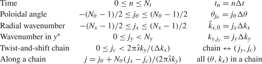
 ). The discrete indices used in this work are defined in table 2. With these definitions, the time derivative of any fluctuating quantity $\varPhi$
 is approximated by

where $\sigma$ is the sign of $\boldsymbol {v}\boldsymbol {\cdot } \hat {\boldsymbol {b}}$
 . Similarly, derivatives in $\theta$
 are approximated by

and all other terms are approximated by

Indices used in discrete notations.

We now use bold-font vector notation for the potential and distribution function, to denote discrete arrays whose indices span every $(\theta ,k_x)$ of a single twist-and-shift chain. Matrices with two such indices are denoted using bold uppercase letters. With this notation, discretising the gyrokinetic equation (2.14) according to (A 1), (A 2) and (A 3) yields

where we have defined the matrices


Finally, the quasineutrality equation, (2.21), is evaluated at time step $n +1$ and written in the discrete form

where we have defined the matrix

The velocity-space integral operator ${\boldsymbol{\mathsf{W}}}$ is defined such that, for any function $\varPhi$
 ,