1. Introduction
Against the backdrop of rapid technological development, wearable exoskeletons have been developed to enhance human capabilities, frequently being used in military applications to enhance soldiers’ endurance and in industrial applications to improve workers’ efficiency [Reference Zeng, Gan and Li1]. Among these devices, lower limb-assisted exoskeletons are crucial, as the hip joint of a lower limb exoskeleton robot is the main load-bearing joint.
The hip joint of a lower limb exoskeleton robot is the main load-bearing joint. The hip joint is a complex system that bears the greatest forces and serves as the crucial connection between the upper and lower limbs [Reference Zhang, Cao, Chen, Yu, Wu and Meng2]. Its indispensable role is highlighted by its contribution of 45% of the mechanical power and the largest joint mechanical work during a gait cycle [Reference Chen, Zi, Qin and Pan3]. Therefore, the design of effective hip joint assistance mechanisms is a key challenge in the development of lower limb exoskeletons. Many studies have been conducted on hip joint assistive exoskeletons both domestically and internationally. Current research on hip joint assistive exoskeletons can be broadly divided into active and passive systems. Active/rigid exoskeletons, such as the hydraulically driven Human Universal Load Carrier (HULC) [Reference Kazerooni, Steger and Huang4–Reference Sankai6] and the complex HAL-5 [Reference Zhang, Yang and Chen7], offer high load-bearing capacity and multi-dimensional motion mimicking natural gait. However, these systems generally face limitations including short endurance (e.g., HULC’s 1-h limit), high technical complexity, and high costs. Furthermore, rigid systems like REWALK [Reference Zoss8, Reference Toyama and Yamamoto9], while lightweight due to carbon fiber, often only support basic walking with short battery life. Passive and soft exoskeletons offer lightweight, lower-cost, and comfortable alternatives. For instance, soft exoskeletons or lightweight elastic garments [Reference Yang, Park, Kim, Park and Lee10] utilize flexible materials [Reference Cao, Chen, Hu, Fang and Wu11] or optimized springs to reduce metabolic costs [Reference Shen, Sam, Allison and Cui12] (e.g., up to 15.28% reduction under a 15 kg load). More recent advances in soft exoskeletons have shown improvements in control strategies and energy transfer efficiency, aiming to increase the effective assistive torque and adaptability for various gaits [Reference Williams, Cuddeback, Fang, Colley, Enlow, Cox, Pridham and Lerner13–Reference Sun, Deng, Wang, Zhou and Song15]. However, reconciling high assistive torque with low weight and true multi-mode adaptability remains a critical challenge for most soft systems.
Based on the limitations of existing active and passive systems, a significant challenge remains: the hip joints of current lower limb-assisted exoskeletons suffer from single mechanisms, few degrees of freedom, and limitations in the types of gaits they can assist. Modern exoskeleton applications require assistance not just for simple walking but for a variety of complex and alternating motions (e.g., running, carrying, climbing), a concept known as polymorphism [Reference Siviy, Baker, Quinlivan, Porciuncula, Swaminathan, Awad and Walsh16]. Therefore, there is an increasing demand for an exoskeleton capable of providing effective and adaptable assistance across multi-mode operations. To address the challenge of achieving multi-mode assistance, this paper proposes a novel double-cam hip joint assist mechanism. This mechanism utilizes a passive drive, employing a double cam and two rectangular compression springs with different stiffness to satisfy the varying assistance requirements across multiple gaits (walking, running, and carrying). Our methodology involves (1) using OpenSim for biomechanical simulation to obtain multi-mode hip joint data, (2) planning cam contours and determining spring stiffness, and (3) verifying the assistance through a human–machine coupling model and muscle power analysis.
2. Structural design
2.1. Analysis and simulation of walking, running, and carrying gait
Walking is the most common and basic gait of the human body [Reference Quínto, Pinheiro, Gonçalves, Roupa, Simoes and da Silva17]. As shown in Fig. 1, the walking gait cycle is universally divided into two primary phases: the support phase (or stance phase) and the swing phase. This fundamental classification is standard in biomechanics, with the support phase accounting for approximately 60% of the cycle and the swing phase accounting for approximately 40% [Reference Perry and Burnfield18].
Walking gait cycle [Reference Yeung19].

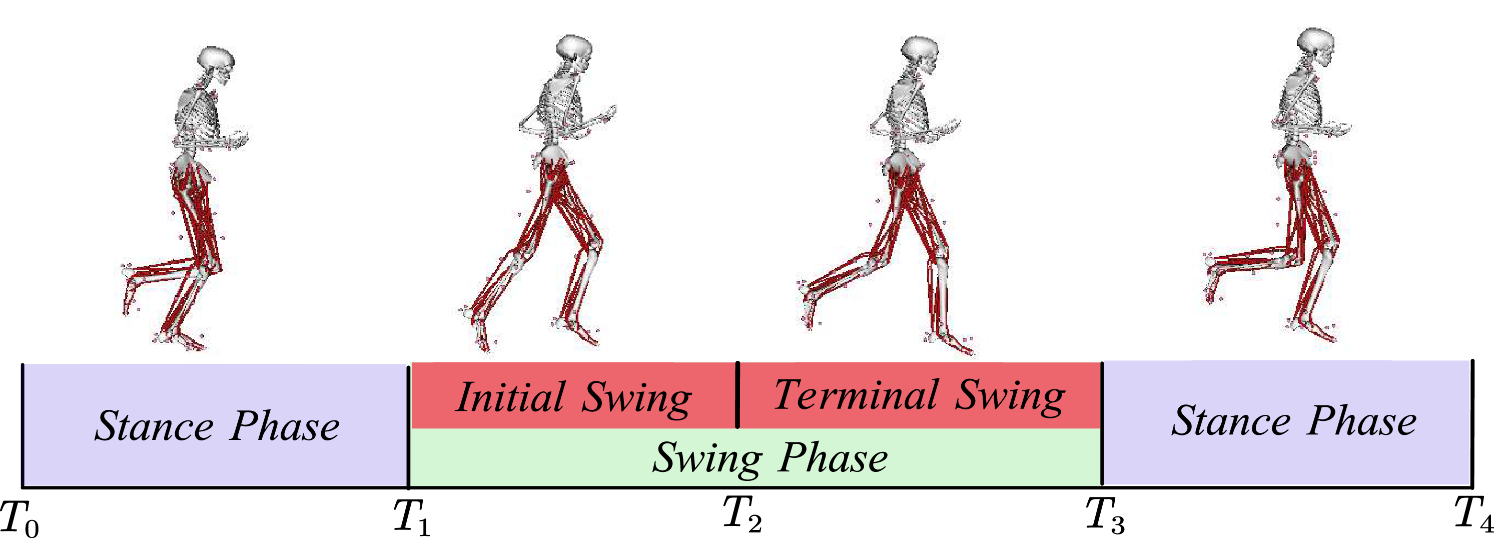
Compared to walking, running involves larger stride lengths, higher step frequencies, and more intense shifts in the body’s center of gravity. The changes in leg movement during running can be divided into the following time periods, as shown in Fig. 2: support phase, swing phase (initial swing phase, terminal swing phase), and support phase. For both walking and running, the muscles around the hip joint, such as the sartorius muscle, gracilis muscle, and iliopsoas muscle, have higher metabolic rates.
Running gait cycle.
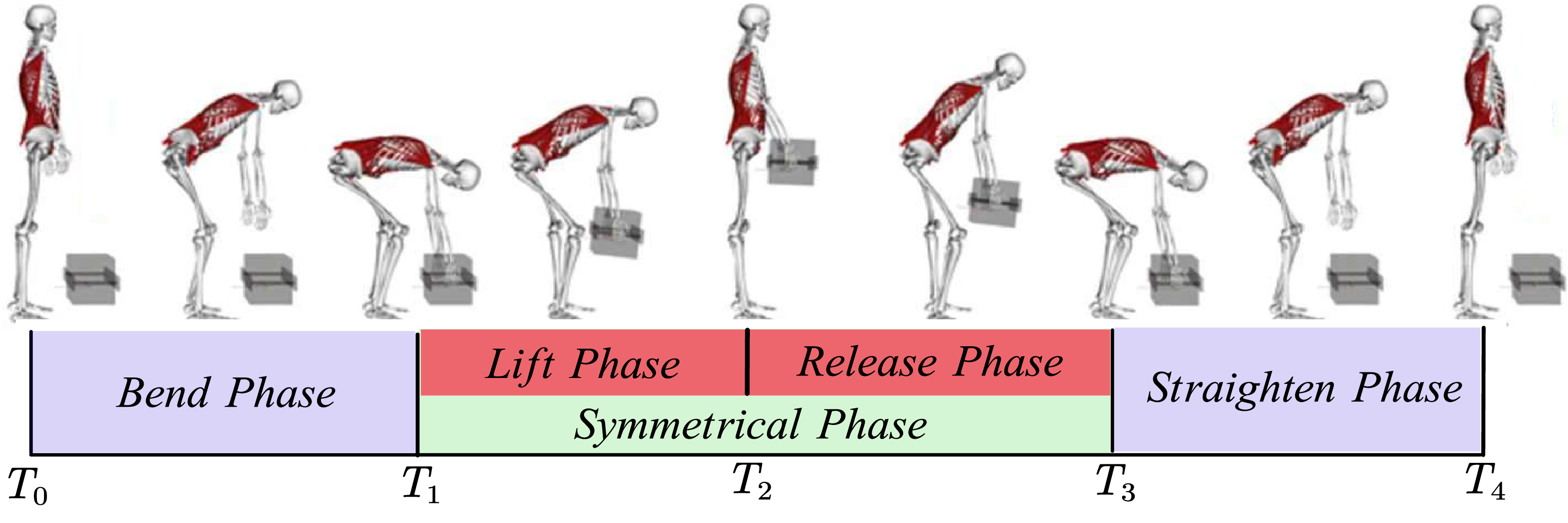
Carrying is a common action during the transfer of objects, as shown in Fig. 3. In the carrying gait, the gait cycle can be divided into the bending phase, the symmetrical moving phase, and the straighten phase, with the symmetrical phase further divided into the lifting phase and the release phase. Within a single cycle, these phases account for 26%, 24%, 24%, and 26%, respectively. During this process, the metabolic rate of the muscles in the waist and back, such as the erector spinae muscles, rectus abdominis muscles, and latissimus dorsi muscles, increases significantly, and there are noticeable changes in muscle length.
Carrying gait cycle [Reference Akhavanfar, Uchida, Clouthier and Graham20].
Polymorphism analysis model.
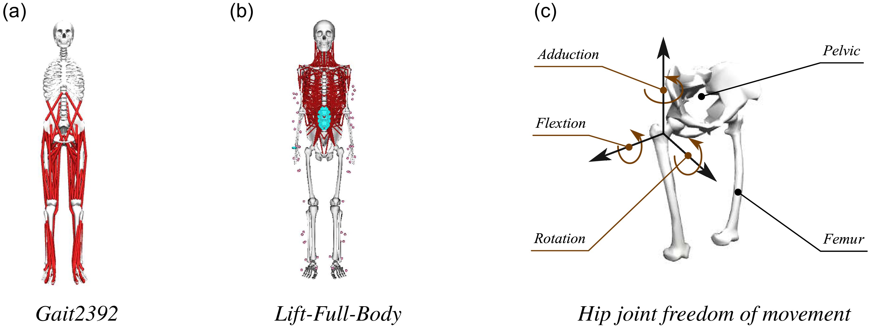
The models used (Gait2392 and Lift-Full-Body) are validated, publicly available models from the OpenSim (SimTK) repository, as shown in Fig. 4. The required experimental motion data (kinematics and ground reaction forces) for simulating walking, running, and carrying gaits were sourced directly from the standard datasets associated with these models within the SimTK repository (e.g., the “Lifting” motion data for the Lift-Full-Body model). These datasets represent pre-validated, generalized human motion trials, thus eliminating the need for new experimental data collection for model initialization. The selection of these standardized and validated datasets enhances the reliability and repeatability of the simulation results.
In OpenSim, walking, running, and carrying gaits were loaded for simulation, and the hip joint rotation angles were analyzed under multiple gaits. The three degrees of freedom of the hip joint rotation angles are shown in Fig. 5. It can be seen that the range of hip joint flexion/extension angles is most significant during walking, running, and carrying gaits.
Three degrees of freedom rotation diagram of a polymorphic hip joint.

Simulation analysis of walking gait, running gait, and carrying gait all correspond to a single gait cycle of the human body. During carrying gait, the hip joint undergoes two symmetrical “peaks” in its flexion/extension angle (
 $\theta _{Hip}$
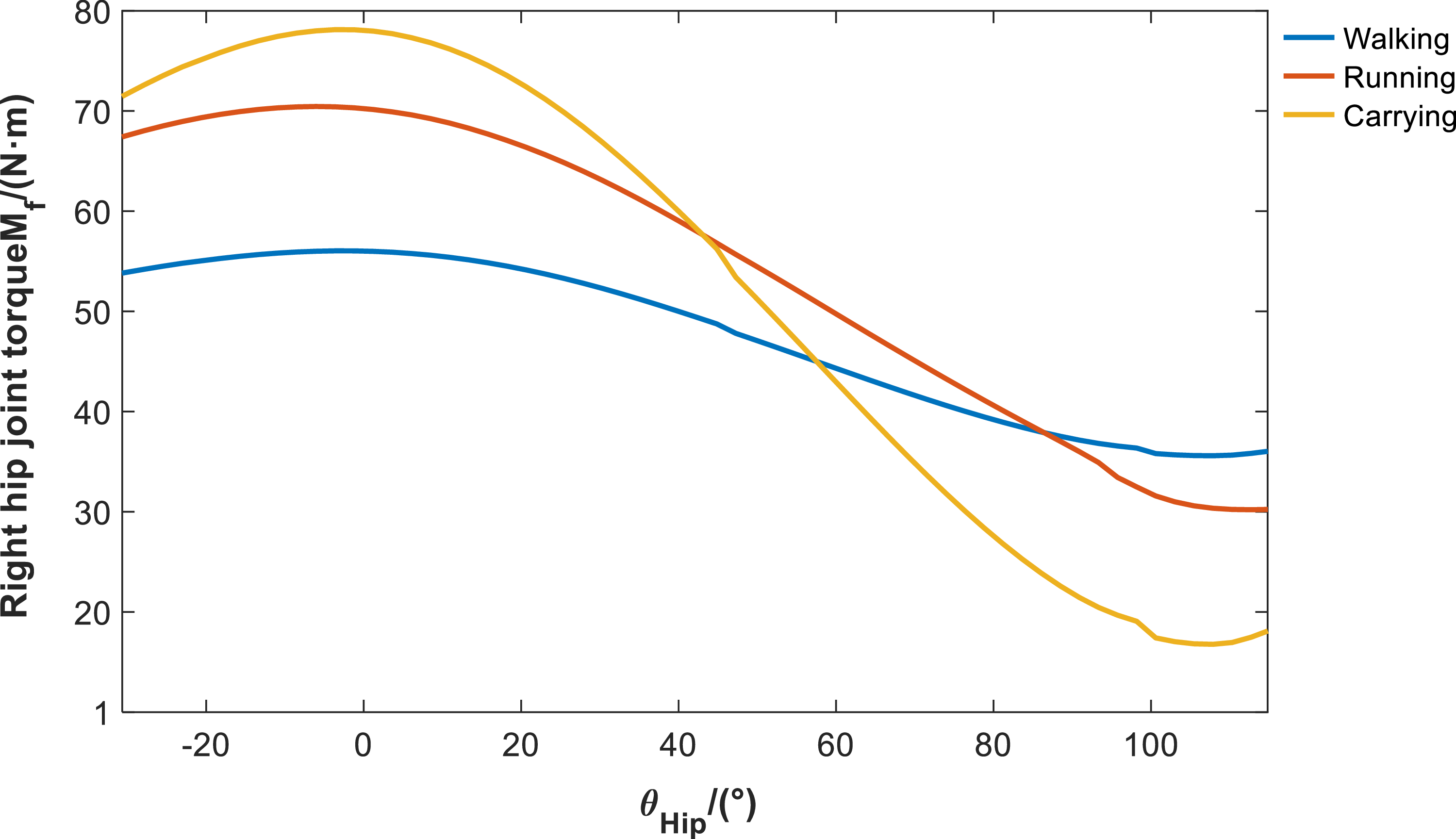
), indicating that it goes through a bending phase-straightening phase-bending phase-straightening phase. The first half of this cycle is the loading phase, while the second half is the unloading phase. The significant changes in the hip joint flexion/extension angle during multi-mode provide design insights, suggesting that the passive components of the hip joint should be positioned along its flexion/extension axis. This arrangement allows significant changes in joint angle during active movement to drive the deformation of elastic elements, thereby facilitating assistance. Figure 6 shows the torque
 $M_{f}$
acting on the right hip joint in the flexion/extension direction during the multi-mode experiment. This study’s dual-wheel auxiliary mechanism is designed to meet the demands of three multi-modal gaits: walking, running, and carrying heavy loads. Consequently, the torque-angle curve shown in Fig. 6 reflects the composite requirements derived from superimposing all three gaits. Specifically, normal walking (see Fig. 5(a)) corresponds to a hip flexion–extension angle range of approximately
 $[{-}30^\circ , 20^\circ ]$
, which primarily aligns with the left portion of the Fig. 6 curve. The curve’s extension up to a
 $100^\circ$
angle range is contributed entirely by the carrying gait. In the carrying gait, the human body performs a large stooping motion to lift heavy objects from the ground, causing the hip flexion angle to significantly exceed
 $100^\circ$
(see Fig. 5(c)). Therefore, the angle range of
 $[{-}20^\circ ,100^\circ ]$
shown in Fig. 6 represents the required design envelope that this mechanism must satisfy to achieve multi-modal assistance, and it does not solely represent the single walking range of a healthy population.
Polymorphic hip flexion/extension directional torque.

It can be observed that in the multi-mode condition, the torque reaches its peak when the hip joint is in the balanced position, when no flexion/extension occurs. The peak torque is highest during the carrying gait phase, followed by running and walking.
2.2. Exoskeleton structure design
Based on the hip joint torque analysis in Section 2.1, during continuous walking and running, the internal torque is greatest when the hip joint is close to aligning with the vertical axis on a single leg. Based on this design principle, a double-cam assist mechanism is proposed to provide an assistive torque when the hip joint is at a flexion–rotation angle of 0 degrees.
In previous studies, researchers have attempted to combine torsion springs and cams to provide torque. However, the torque accumulation in this approach is unidirectional and only effective during walking or running-like gaits, failing to meet the assistive requirements for other types of locomotion beyond walking and running. Therefore, this study proposes the design of two disc-shaped cams, referred to as double cam, and equipped with two rectangular compression springs of different stiffness to accommodate the varying requirements for exoskeletal assistance across different gait patterns. Cam 1 functions during walking, running, and carrying gait patterns, with a higher operational frequency, larger preload, and more complex changes. It is positioned on the side distant from the hip joint for ease of installation. Cam 2 functions during walking and running, positioned on the inner side with a smaller preload compared to Cam 1. Its axonometric view is shown in Fig. 7. Considering the machining accuracy of the cam profiles, both cams 1 and 2 are equipped with locating reference holes and reference grooves.
Axonometric view of double-cam mechanism.

Figure 8 shows the overall structure of the hip exoskeleton. The hip exoskeleton primarily consists of the double-cam mechanism, thigh follower rod, connecting plate, and fixed plate shown in Fig. 8. The connecting plate secures both sides of the hip exoskeleton to the rear support waist rod. The double-cam mechanism is fixed to the connecting plate via the fixed plate using set screws. The thigh follower rod is secured to the thigh via the thigh fixation fixed to it.
Polymorphic hip flexion/extension directional torque.

When rotating the thigh rod with one leg, the length of the springs in the follower systems 1 and 2 on the thigh rod changes under the action of the cam profiles 1 and 2, generating two spring forces. These spring forces produce a torque at the hip joint center, thereby providing assistance in multiple positions as the hip joint angle
 $\theta _{Hip}$
changes.
Double-cam structure design.

As shown in Fig. 9(a) and (b), the double-cam mechanism is tangentially fixed to the fixed plate via slotted shaft holes and axially fixed via locking nuts, ensuring that the double-cam mechanism, fixed plate, and connecting plate are all securely connected to the rear support waist rod. The double-cam mechanism features two layers of flat disc-shaped cams. The layer furthest from the body on the coronal axis is referred to as cam 1, while the layer closest to the body is referred to as cam 2. Each cam has a follower system, which consists of a rectangular spring, a slide groove, and a follower. The slide groove is inserted into the thigh rod and secured with set screws, with the follower placed inside the groove. The follower is in close contact with the cam profile under the preload of the rectangular spring.
2.3. Double-cam mechanism contour design
The design process for a cam mechanism generally includes the following steps:
1) Select the type of cam mechanism. Considering factors such as weight, space, and manufacturing difficulty, this paper selects a planar cam mechanism as the basic structural form and a cam-driven translating follower as the specific form for the exoskeleton cam system. The follower is chosen with a circular end, which produces low noise and ensures smooth transitions during contour curve changes.
2) Determine the basic dimensions of the cam mechanism. In this paper, the basic geometric dimensions of the double cam are selected based on the cavity dimensions. According to the empirical calculation method [Reference Shao, Xiang, Liu and Li21]:
 \begin{equation} \begin{aligned} & R_b(Theoretical\,base\,circle\,radius) \\[5pt] & =d/2(Cam\,shaft\,diameter)+Safety\,clearance \end{aligned} \end{equation}
For cam 1, which has a more complex contour profile, to ensure its stiffness, the base radius
 $R_{b1}$
is preliminarily selected as 20 mm using Eq. (1), with a maximum lift of 30 mm; for cam 2, which has a simpler operating profile, the base radius
 $R_{b2}$
is selected as 18 mm using Eq. (1), and the maximum lift is 20 mm. Based on experience, the roller radius
 $r_{b1}=r_{b2}=6mm$
is selected. Next, the offset is selected. The assist principle of the double-cam mechanism is to generate a torque around the hip joint center. This critical point requires that the offsets corresponding to cams 1 and 2 be symmetrically arranged along the sagittal axis. Additionally, considering the forces acting on the fixed plate, they should also be symmetrically arranged vertically. Cam 1 experiences greater forces, so to fully utilize the spring force to generate torque, offset
 $e_{1}$
should be slightly larger than offset
 $e_{2}$
. For testing,
 $e_{1}$
is set to 6 mm and
 $e_{2}$
to 5 mm.
3) Select the motion law of the follower. The motion laws of translating followers mainly include several common types, such as uniform motion, uniform acceleration and deceleration motion, sinusoidal acceleration law, and polynomial law, etc. [Reference Shao, Xiang, Liu and Li21, Reference Chang, Hu and Chang22]. Among them, the sinusoidal acceleration law is particularly suitable for the periodic flexion motion of the human hip in multiple states. The displacement
 $s_{\mathrm{p}}$
, velocity
 $\nu _{\mathrm{p}}$
, acceleration
 $a_{\mathrm{p}}$
, and displacement change
 $j_{\mathrm{p}}$
during the push phase of the sinusoidal acceleration pattern are generally expressed by Eq. (2).
 \begin{equation} \begin{cases} \begin{aligned} s_{\mathrm{p}}& =h\left (\frac {t}{t_{\mathrm{h}}}-\frac {1}{2\pi }\sin \frac {2\pi t}{t_{\mathrm{h}}}\right ) \\[5pt] \nu _{\mathrm{p}}& =\frac {h}{t_{\mathrm{h}}}\left (1-\cos \frac {2\pi t}{t_{\mathrm{h}}}\right ) \\[5pt] a_{\mathrm{p}}& =\frac {2\pi h}{t_{\mathrm{h}}^2}\sin \frac {2\pi t}{t_{\mathrm{h}}} \\[5pt] j_{\mathrm{p}}& =\frac {4\pi ^2h}{t_{\mathrm{h}}^3}\cos \frac {2\pi t}{t_{\mathrm{h}}} \end{aligned} \end{cases} \end{equation}
During the return phase, the expressions of various variables are similar to those in the forward phase. The velocity
 $\nu _{\mathrm{r}}$
, acceleration
 $a_{\mathrm{r}}$
, and jump
 $j_{\mathrm{r}}$
are opposite to those in the forward phase, and the displacement
 $s_{\mathrm{r}}$
is given by Eq. (3).
 \begin{equation} s_{\mathrm{r}}=h\left (1-\frac {t}{t_{\mathrm{h}}}+\frac {1}{2\pi }\sin \frac {2\pi t}{t_{\mathrm{h}}}\right ) \end{equation}
4) Divide the motion stages and plan the displacement of the follower. The double-cam mechanism requires the motion stages to be divided separately for cams 1 and 2 in order to achieve coordinated operation of the double cam in the three gaits of walking, running, and carrying.
As shown in Fig. 10(a) and (b), the two disks represent the angular divisions of the cam, and the red dots indicate the assist switching points for different gait states. For the motion phase division of cam 1, as the disk rotates, the end of disk 1 starts from the initial contact point and sequentially passes through three assist switching points. When passing through the first assist switching point, the rotation angle of the disk is
 $\theta _{walk}$
; when passing through the second assist switching point, the rotation angle of the disk is
 $\theta _{run}$
; and when passing through the third assist switching point, the rotation angle of the disk is
 $\theta _{carry}$
. Let
 $\theta _{walk}$
,
 $\theta _{run}$
, and
 $\theta _{carry}$
represent the maximum hip joint flexion angles for walking, running, and carrying gait, respectively. For walking and running gait, when
 $0\lt \theta _{Hip}\lt \theta _{walk}$
, cam 1 acts on the circular end 1 to gradually release the preload force as hip joint flexion assistance. When
 $\theta _{walk}\lt \theta _{Hip}\lt \theta _{run}$
, cam 1 acts on the circular end 1 to transition, continuing to release spring force; the circular end continues to rotate. For the carrying gait, when
 $\theta _{run}\lt \theta _{Hip}\lt \theta _{carry}$
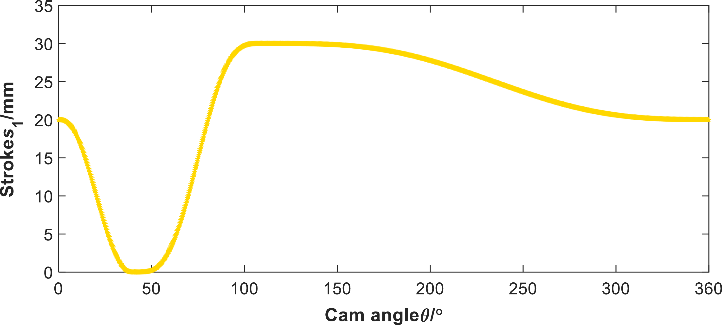
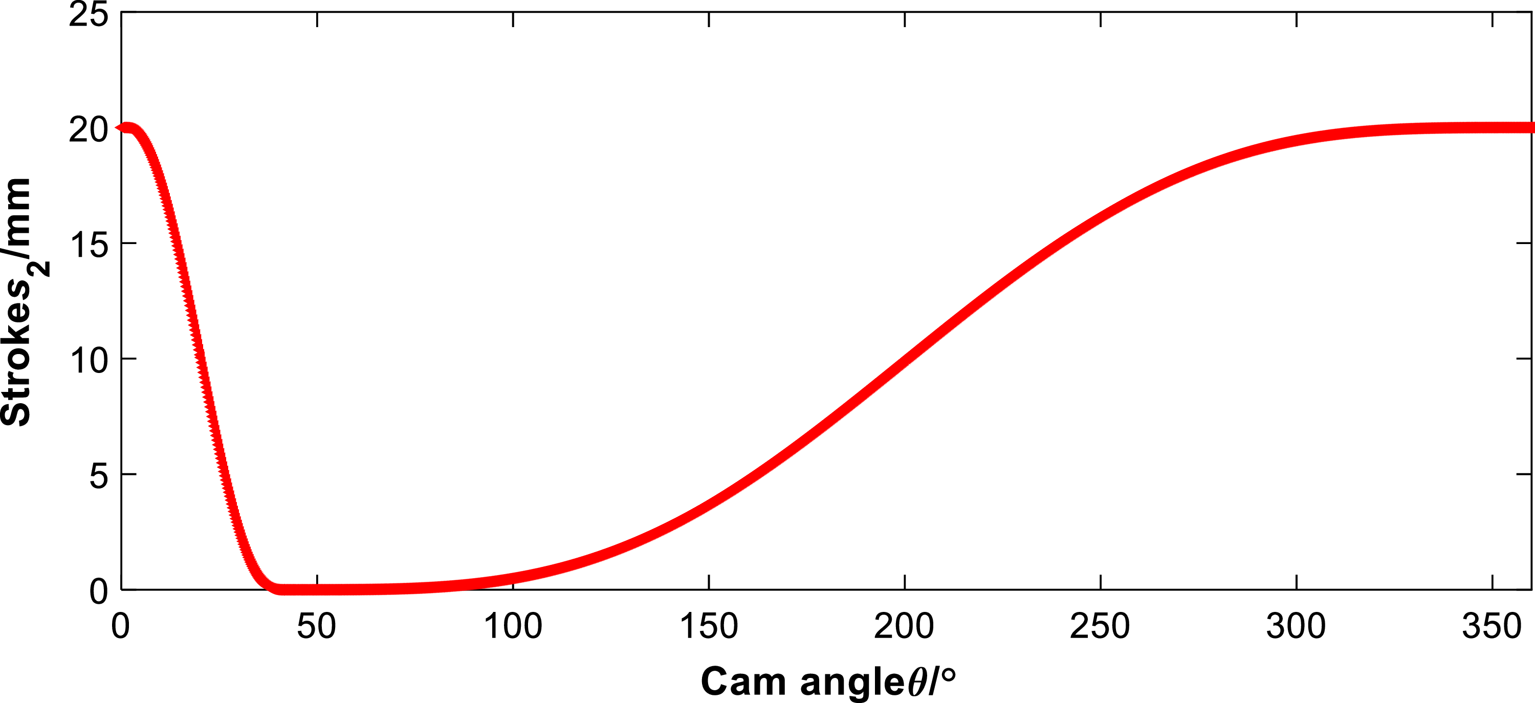
, the preload gradually increases, accumulating elastic force for the human body during the straighten phase of the carrying gait. The design process for cam 2 is similar but does not include the assist switching point for the carrying gait. After determining the cam profiles of cam 1 and cam 2, set the interpolation conditions and boundary conditions for the circular end travel distances
 $s_{1}$
and
 $s_{2}$
of cam 1 and cam 2 as shown in Table I. Solving the equations in the table yields the travel distance variation curves
 $s_{1}$
and
 $s_{2}$
of the two circular ends of the double cam, as shown in Figs. 11 and 12.
5) Solve the cam profile curve. After obtaining the stroke changes of the two circular ends of the double cam, the profile curves of cams 1 and 2 in the double cam can be calculated using the reverse analysis method. Figure 13 shows a simplified diagram of the cam profile for the translating follower in contact with the circular end, obtained using the reverse method.
Double-cam interpolation conditions and boundary conditions.

Double-cam motion phase planning diagram.

Cam 1 stroke diagram.

Cam 2 stroke diagram.

Reverse analysis method.

In the
 $\text{XOY}$
plane shown in Fig. 13, the formula for calculating the cam theory profile is:
 \begin{equation} \begin{cases} x=-e\cos \varphi -(s+s_0)\sin \varphi \\[5pt] y=-e\sin \varphi +(s+s_0)\cos \varphi & \end{cases} \end{equation}
In this equation,
 $\varphi$
represents the cam angle,
 $\mathrm{s}$
represents the stroke, and
 $s_{0}$
represents the initial displacement. Substituting
 $s+s_{0}$
into the equation and solving it in MATLAB yields the profile curves of cams 1 and 2. It is worth noting that the
 $\text{X}$
-coordinate of the contour of cam 2 is opposite to that of cam 1. Then, solve for the actual contour of the cam using Eq. (6).
 \begin{equation} \begin{cases} \begin{aligned} x^{\prime }& =\left (e-\frac {\mathrm{d}s}{\mathrm{d}\varphi }\right )\mathrm{sin}\varphi -\left (s_0+s\right )\mathrm{cos}\varphi \\[5pt] y^{\prime }& =\left (e-\frac {\mathrm{d}s}{\mathrm{d}\varphi }\right )\mathrm{cos}\varphi -\left (s_0+s\right )\mathrm{sin}\varphi \\[5pt] \gamma & =\arctan (\frac {y^{\prime }}{x^{\prime }}) \end{aligned} \end{cases} \end{equation}
 \begin{equation} \begin{cases} x_K=x-r_b\cdot \sin \gamma \\[5pt] y_K=y+r_b\cdot \cos \gamma & \end{cases} \end{equation}
 $(x_{K},y_{K})$
represents the actual contour of the double cam. These curves (Fig. 14) are generated based on the selected base dimensions:
 $R_{b1}=20 \text{ mm}$
,
 $e_1=6 \text{ mm}$
for cam 1, and
 $R_{b2}=18 \text{ mm}$
,
 $e_2=5 \text{ mm}$
for cam 2, with a uniform roller radius of
 $r_{b1}=r_{b2}=6 \text{ mm}$
(as detailed in Section 2.3).
Double-cam profile diagram.

2.4. Selection of spring stiffness and analysis of assist torque
In the rigid system of a double-cam system, once the basic dimensions and contour lines of the cam are determined, the spring stiffness of the translating follower is not only a key factor in providing assistance but also an important factor influencing the smoothness of multi-mode assistance in hip joint exoskeletons. In the following section, we will optimize the spring stiffness of the hip joint exoskeleton from the perspectives of the d’Alembert principle and elastic dynamics.
Equivalent kinetic modeling of multi-mode boost switching.

Assume that the forward rotation angle of the human hip joint is
 $\delta$
, and
 $0\lt \delta \lt \theta _{run}$
. The length release of cams 1 and 2 corresponding to angle
 $\delta$
is
 $C_i(i=1,2)$
. At this point, the cam mechanism generates an assistive torque due to the slope of the contour surface and the preload force, and the equilibrium equation is:
 \begin{equation} \begin{aligned} & k_{S1}C_{1}e_{1}+k_{S2}C_{2}e_{2}+\tau _{m}=\tau _{G}+J_{femur}a, \\[5pt] & C_{i}=s_{i}(\delta )\quad i=1,2. \end{aligned} \end{equation}
Similarly, for angle
 $\delta _{1}$
, it is worth noting that
 $\theta _{run}\lt \delta _{1}\lt \theta _{carrry}$
, then we have:
 \begin{equation} \begin{aligned} & k_{S1}C_{1}e_{1}+k_{S2}C_{2}e_{2}+\tau _{m}+\tau _{G}=J_{femur}a_{1}, \\[5pt] & C_{i}=s_{i}(\delta _{1})\quad i=1,2. \end{aligned} \end{equation}
At this point,
 $k_{S2}C_2e_2\approx 0$
. The reliance method can only solve the numerical open intervals of
 $k_{S1}$
and
 $k_{S2}$
, but cannot solve their optimal values. Therefore, it is necessary to establish equations based on the elastic dynamics of cam mechanisms with compliance. As shown in Fig. 15(a), according to the principle of mass conservation in mechanical dynamics, the mass of the translating follower is uniformly distributed at both ends, that is:
 \begin{equation} \begin{aligned} & m_{e1}=\frac {1}{2}m_{O1}+\frac {1}{6}m_{k1},m_{e2}=\frac {1}{2}m_{O2}+\frac {1}{6}m_{k2}, \\[5pt] & \frac {1}{k_{e1}}=\frac {1}{k_1}+\frac {1}{k_{C1}}+\frac {1}{k_{S1}},\frac {1}{k_{e2}}=\frac {1}{k_2}+\frac {1}{k_{C2}}+\frac {1}{k_{S2}}. \end{aligned} \end{equation}
Establish elastic dynamics equations separately:
 \begin{equation} \begin{aligned} & m_{e1}\ddot {y}_2=k_{e1}(s_1-y_1)-k_{\mathrm{S1}}y_1-F_{P1}+G_1, \\[5pt] & m_{e2}\ddot {y}_2=k_{e2}(s_2-y_2)-k_{\mathrm{S2}}y_2-F_{P2}-G_2. \end{aligned} \end{equation}
 $F_{Pi}$
and
 $G_{i}$
are both low-frequency static loads that only cause static deformation. During the transition state of the cam profile curve, they are considered vibration analysis scenarios and are therefore neglected. The stiffness of the compression springs is mapped to the equivalent stiffness and is also neglected. Cams 1 and 2 have different basic dimensions. To facilitate unified analysis, dimensionless expressions are used:
 \begin{equation} \ddot {Y}_1+(2\pi \lambda _1)Y_1=S_1,\ddot {Y}_2+(2\pi \lambda _2)Y_2=S_2. \end{equation}
 $\lambda _i=t_h^i/t_0^i,t_0^i=2\pi /\omega _n^i,\omega _n^i=\sqrt {k_{ei}/m_{ei}}$
, it is worth noting that cam 1 has two rise times for running gait and carrying gait. In order to obtain a smaller equivalent stiffness, the rise time of the carrying gait is selected as
 $t_{h}^1$
, then:
 \begin{equation} \begin{aligned} & \lambda _i=\frac {t_h^i}{2\pi }\sqrt {k_{ei}/m_{ei}}\quad (i=1,2), \\[5pt] & k_{ei}=\frac {1}{k_i^{-1}+k_{Ci}^{-1}+k_{Si}^{-1}}. \end{aligned} \end{equation}
When the double cam is in the return stroke, push stroke, or rest phase, the above equation is in the main oscillation phase. When the contour curve of any cam is in the state transition, the excitation
 $S(T)=0$
. Additionally, the main oscillation phase
 $Y_{i}$
is related to the residual oscillation phase
 $Y_{ri}$
, where
 $Y_{ri}=Y_i-1$
. Therefore, the dynamic differential equations for cams 1 and 2 are:
 \begin{equation} \begin{aligned} & \ddot {Y}_{r1}+(2\pi \lambda _1)^2Y_{r1}=0,\ddot {Y}_{r2}+(2\pi \lambda _2)^2Y_{r2}=0, \\[5pt] & Y_{r1}(T)=Y_{r2}(T)=\frac {1}{\pi }\frac {1}{\lambda ^{3}-\lambda }\sin \pi \lambda \cos [\pi \lambda (2T-1)]. \end{aligned} \end{equation}
The maximum amplitude of
 $Y_{ri}$
should be as small as possible, and
 $T\in [0,1]$
, so this problem can be regarded as an optimization problem of
 $\lambda$
and
 $T$
with respect to the function
 $Y_{ri}$
.
 \begin{equation} \begin{aligned} & \min \max (Y_r) \\[5pt] & subject\,to\;:\;T\in [0,1],\lambda _i\gt 0(i=1,2) \\[5pt] & k_{S1}C_1e_1+k_{S2}C_2e_2+\tau _m=\tau _G+J_{femur}a \\[5pt] & k_{S1}C_1e_1+k_{S2}C_2e_2+\tau _m^{\prime }+\tau _G^{\prime }=J_{\mathrm{\,femur}}a^{\prime } \end{aligned} \end{equation}
The Nelder–Mead method was used to solve the problem in MATLAB, with a step size of 0.1. The distribution of each variable is shown in Fig. 16.
Optimization results.

It is desirable to select a smaller equivalent stiffness at smaller residual amplitude values. Since
 $\lambda _i\sim k_{ei}\sim k_{Si}$
, the stiffness of the two springs can be selected and calculated:
 \begin{equation} k_{S1}=372.17N/m,k_{S2}=187.11N/m. \end{equation}
When the human body is walking or running, the single leg is in the swing phase, and the hip joint is at an angle of
 $\theta _{Hip}$
. The torque generated by the spring is defined as:
 \begin{equation} \begin{aligned} M_{h} & =(F_1-k_{S1}\cdot s_1(\theta _{Hip}))\cdot e_1 \\[5pt] & +(F_2-k_{S2}\cdot s_2(\theta _{Hip}))\cdot e_2 \end{aligned} \end{equation}
where
 $F_1$
and
 $F_2$
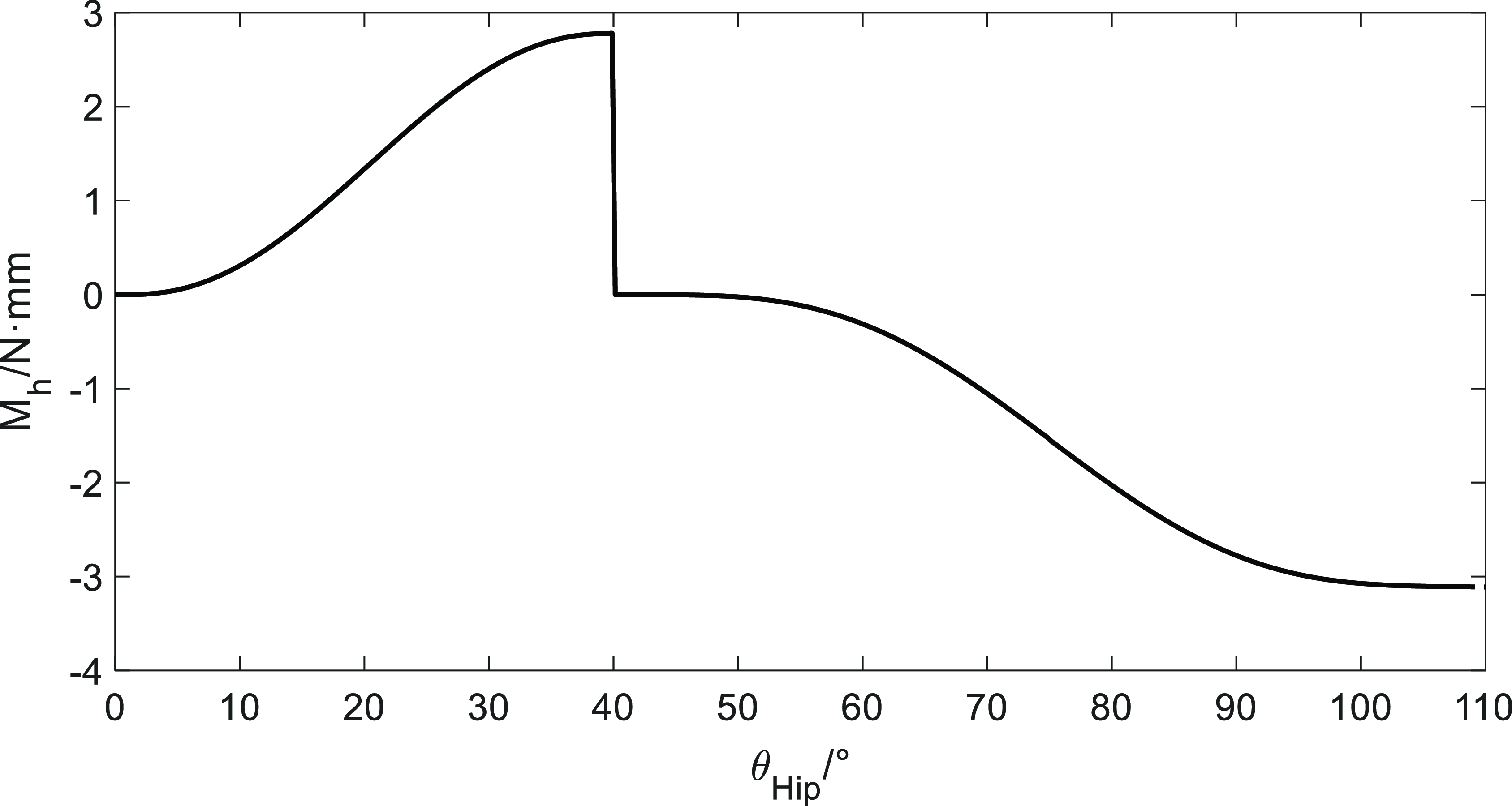
are the preload forces of rectangular springs 1 and 2, respectively. The relationship curve between
 $M_{h}$
and
 $\theta _{Hip}$
is shown in Fig. 17. It is observed in Fig. 17 that the generated torque
 $M_{h}$
exhibits a sharp discontinuity at
 $\theta _{Hip}=40^\circ$
. This angle corresponds to the transition point between the walking/running assistance phase (where
 $s_i$
decreases to zero) and the subsequent carrying gait phase transition, as defined by the phase division in Fig. 10 and Table I. While the chosen Sinusoidal Acceleration Law ensures continuity of displacement and velocity at this juncture, the sudden change in the required acceleration profile (i.e., the torque required by the spring system) results in a theoretical discontinuity in the jerk, leading to the sharp drop in
 $M_{h}$
. Although this sharp transition is a theoretical limitation of the segmented profile design, the practical application (e.g., machining constraints and roller radius) naturally smooths the profile. For future optimization, a higher-order polynomial function will be used to ensure the continuity of the jerk (third derivative) across all phase transition points, thus eliminating this theoretical "infinite stiffness" issue and minimizing dynamic impact.
 $M_{h}$
-
 $\theta _{Hip}$
curve diagram.

Perform a positive analysis along the
 $\theta _{Hip}$
-axis for the
 $M_{h}$
-
 $\theta _{Hip}$
curve. During walking and running gait,
 $0\lt \theta _{Hip}\lt \theta _{run}$
, when the single leg is in the swing phase, the hip joint flexion angle is
 $\theta _{Hip}$
, and
 $\theta _{Hip}$
gradually increases from
 $0\circ$
to
 $\theta _{run}$
. At this point,
 $M_{h}$
gradually increases, causing hip joint flexion and generating a torque at the center of hip joint flexion, which assists the single-leg swing phase. In the carrying gait,
 $\theta _{run}\lt \theta _{Hip}\lt \theta _{carry}$
, as
 $\theta _{Hip}$
gradually increases from
 $\theta _{run}$
to
 $\theta _{carry}$
,
 $M_{h}$
acts as a counter-torque, resisting hip joint flexion, and maintaining stability as the gravitational potential energy of the upper body decreases. While the
 $M_{h}$
-
 $\theta _{Hip}$
curve can qualitatively indicate assistance, this isolated structural analysis cannot determine the precise interaction dynamics between the exoskeleton and the human limb. Therefore, a human–machine coupling model must be established for further analysis.
3. Human–machine coupling model
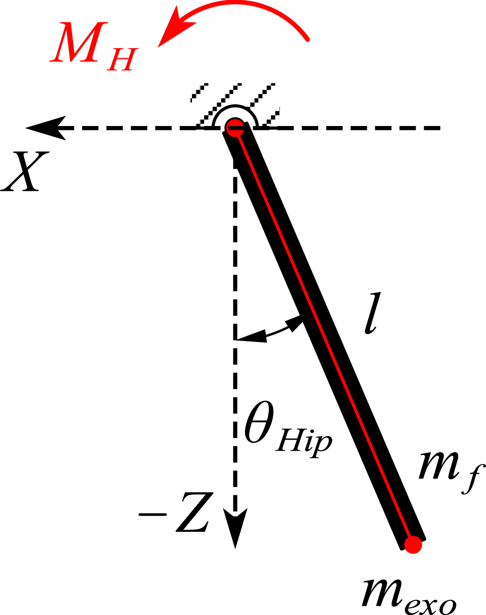
To investigate whether a hip exoskeleton can provide passive assistance for hip movement, it is necessary to establish a human–machine coupling model using dynamic analysis methods. The use of the Lagrangian dynamics method to analyze the assistive properties of hip exoskeletons offers several advantages. According to multi-mode analysis, the kinematics and dynamics of both legs during walking and running exhibit a certain degree of symmetry. Therefore, the human–machine coupling model can be simplified [Reference Wu, Zeng, Ruan, Guo, Yang, Jing and Yao23], resulting in the model shown in Fig. 18.
Hip human–machine coupling equivalent model.

Assume that the single leg and the exoskeleton can be equivalently modeled as a rigid rod of length
 $\mathit{l}$
, with the exoskeleton rigidly connected to the single leg. The mass of the hip exoskeleton
 $m_{exo}$
and the mass of the single leg
 $m_{f}$
are both concentrated at the end of the rod, that is, at the theoretical knee joint. When the single leg and the hip exoskeleton are in the swing phase, the hip joint flexes forward by
 $\theta _{Hip}$
. According to the Lagrange function
 $\mathit{L}$
, which represents the kinetic energy minus the potential energy of the human–machine system:
 \begin{equation} L=T-V \end{equation}
Substitute the kinetic and potential energies of the human–machine coupling into the Lagrange function:
 \begin{equation} \begin{aligned} & T=T_f+T_{exo}=\frac {1}{2}(m_f+m_{exo})l^2\dot {\theta }_{Hip}^2 \\[5pt] & V=V_f+V_{exo}=-(m_f+m_{exo})gl^2\cos (\theta ) \\[5pt] & L=\frac {1}{2}(m_f+m_{exo})l^2\dot {\theta }_{Hip}^2+(m_f+m_{exo})gl^2\cos (\theta ) \end{aligned} \end{equation}
Due to the unique arrangement of the elastic components of the hip exoskeleton in this paper, the elastic torque
 $M_{H}$
is used to consider the influence of the elastic components. Based on this, the Lagrange equation is:
 \begin{equation} \frac {d}{dt}\left (\frac {\partial L}{\partial \dot {\theta }_{Hip}}\right )-\frac {\partial L}{\partial \theta _{Hip}}=M_h+M_f \end{equation}
Substituting Eq. (18) into the equation, we obtain:
 \begin{equation} (m_f+m_{exo})l^2\ddot {\theta }_{Hip}+(m_f+m_{exo})gl\sin (\theta _{Hip})=M_h+M_f \end{equation}
In Eq. (20),
 $(m_f+m_{exo})l^2$
represents the rotational inertia matrix of the hip joint and exoskeleton in the human–machine system, and
 $(m_f+m_{exo})gl$
represents the coupling matrix between the hip joint and exoskeleton, including centrifugal forces and Coriolis torque matrices. It is clear that these two key matrices are closely related to the mass and length of the human single leg and the hip exoskeleton. By transforming the Lagrange equations, we obtain:
 \begin{equation} \ddot {\theta }_{Hip}+\frac {g}{l}\sin (\theta _{Hip})=\frac {M_h+M_f}{(m_f+m_{exo})l} \end{equation}
Combining the torque
 $M_{h}$
obtained earlier with Eq. (21), we analyze the human body’s multi-mode behavior. Here, g is the gravitational acceleration,
 $\mathit{l}$
is the length of the thigh, and
 $m_f+m_{exo}$
is the mass of the human–machine system. All three physical quantities are constants. Assuming that the
 $\theta _{Hip}$
values are the same for both assisted and unassisted conditions, that is, assuming that the changes in hip joint angles between assisted and unassisted conditions are negligible, we proceed with the following assisted analysis.
During the single-leg swing phase of human walking or running (at this point,
 $0\lt \theta _{Hip}\lt \theta _{run}$
), muscles near the hip joint generate a torque
 $M_{f}$
that causes hip flexion. At this point, the torque
 $M_{h}$
is positive and aligned with the direction of
 $\theta _{Hip}$
(red direction in Fig. 18). Combining Eq. (21) with Fig. 17, the exoskeleton provides a torque to assist leg swinging, with the unassisted
 $\ddot {\theta }_{Hip}$
greater than the assisted
 $\ddot {\theta }_{Hip}$
, indicating exoskeleton assistance. At the end of the single-leg swinging phase during walking or running, the force
 $M_{f}$
acting on the hip joint causes the hip joint angular velocity to gradually decrease and reverse direction. At this point, the torque
 $M_{h}$
remains positive, combining Eq. (21) with Fig. 17, the exoskeleton provides a torque that also reduces the angular velocity of the leg, with the
 $\ddot {\theta }_{Hip}$
without assistance being smaller than the
 $\ddot {\theta }_{Hip}$
with assistance, making it easier for the leg to enter the support phase, and providing deceleration and stability.
For the carrying gait (at this point
 $\theta _{run}\lt \theta _{Hip}\lt \theta _{carry}$
), during the bending phase, muscles near the hip joint generate a torque
 $M_{f}$
that resists hip flexion. This torque
 $M_{f}$
plays a stabilizing role as the upper body center of gravity descends. At this point, combining Eq. (21) with Fig. 17,
 $M_{h}$
is negative, resisting hip flexion, and the
 $\ddot {\theta }_{Hip}$
without assistance is smaller than the
 $\ddot {\theta }_{Hip}$
with assistance. At this point, the hip exoskeleton also plays a stabilizing role. During the straighten phase, muscles near the hip joint generate a moment
 $M_{f}$
that causes hip extension. At this point,
 $M_{h}$
is negative, and the
 $\ddot {\theta }_{Hip}$
without assistance is greater than the
 $\ddot {\theta }_{Hip}$
with assistance, aiding hip extension. During the straighten phase, the muscles provide assistance. In summary, the torque generated by the double-cam mechanism exhibits certain assistive/stabilizing effects during different phases of the multi-mode process.
4. Muscle power analysis
For walking and running simulation experiments, maintain the same process and settings as in Section 2.1 (Model Integration and Co-simulation Details). To obtain the total muscle power with the assistive device, the double-cam mechanism was integrated into the OpenSim environment. This was achieved by:
-
1. Mechanism Modeling: The double-cam mechanism, thigh follower rods, and two rectangular springs were modeled as a simplified mechanical subsystem.
-
2. Integration: The mechanism was rigidly attached to the hip joint axis (flexion/extension) of the Gait2392/Lift-Full-Body model. The influence of the double-cam system was represented by adding two spring elements (using OpenSim’s internal elastic force components) whose forces were applied to the thigh segment via the cam followers.
-
3. Torque Application: The assistive torque
 $M_h$
(derived from the spring forces and cam geometry, as analyzed in Section 2.4) was automatically calculated by OpenSim’s dynamics engine as the joint angle
$\theta _{Hip}$
changed, effectively acting as an external actuator torque on the hip joint.
-
4. Simulation Process: The simulation utilized the Computed Muscle Control (CMC) tool. CMC determined the minimal muscle activation required to achieve the target motion (kinematics from Section 2.1) while factoring in the assistive torque
$M_h$
provided by the integrated spring mechanism. -
5. Output: The total muscle power was then calculated from the reduced muscle activations and the corresponding muscle force and contraction velocity.


Total muscle power diagram for walking and running.

The simulation results for walking and running gait are shown in Fig. 19. As shown in the figure, between 0 s and approximately 0.15 s, passive drive helps maintain the stability of muscle movement. Between approximately 0.15 s and 0.32 s, passive drive significantly reduces the power of the three muscles, performing positive work in place of the muscles and providing assistance. After 0.36 s, the total muscle negative power amplitude of passive drive decreases. When combined with the hip joint flexion angle in Section 2.1, at this point, the passive drive exoskeleton provides deceleration and stability for the end of the hip joint extension movement.
5. Conclusion
This paper successfully utilized a rigorous multi-mode biomechanical simulation framework using OpenSim and validated public models to obtain essential hip joint angle and torque data, which served as the precise reference for the subsequent mechanism design. The result is a novel passive double-cam hip joint assist mechanism. This innovative structure employs two disc-shaped cams and differential stiffness springs, designed via inverse dynamic principles to precisely manage the assistive torque across various phase transition points. The mechanism achieves genuine multi-mode adaptive assistance for walking, running, and carrying gaits, providing precise assistive torque for propulsion and counter-torque for stabilization during high-flexion maneuvers. The efficacy of the design was verified through a human–machine coupling model and comparative OpenSim simulations using the CMC tool. The multi-mode results demonstrate that the cam mechanism exhibits a significant assist effect: During walking gait, the passive drive significantly reduces the total muscle power peak (as shown in Fig. 19(a)). For running gait, the passive drive performs positive work in place of the muscles, with a significant power reduction observed after 0.15 s, while also decreasing the amplitude of muscle negative power after 0.36 s, providing deceleration and stability (as shown in Fig. 19(b)).
We acknowledge that the current study, focusing on design optimization and theoretical validation, lacks empirical verification through physical experimentation. In the absence of device fabrication and real-world trials, our conclusions remain confined to the computational environment. For future work, the immediate priority will be the fabrication and optimization of the double-cam prototype. Subsequent research will focus on comprehensive experimental studies involving human subjects across walking, running, and carrying tasks. This empirical validation will compare measured human metabolic cost and muscle activity (e.g., using electromyography) with our current simulation results, providing definitive proof of the mechanism’s multi-mode assistive efficacy and addressing the stability concerns related to the cam switching points.
Beyond validation, future work will explore the integration of the double-cam mechanism with external components to create a hybrid system. This could involve combining the passive torque profile with lightweight electrical actuators to supplement peak power needs or incorporating smart materials (such as shape-memory alloys or variable stiffness elastomers) to allow for real-time adaptation of the cam’s geometric parameters or spring stiffness (
 $k_S$
). Such a hybrid approach could retain the energy efficiency of passive design while achieving the precise, active control required for complex terrain or highly individualized rehabilitation protocols.
Data availability statement
The datasets generated and/or analyzed during the current study are available in the [SimTK] repository, accessible via https://simtk.org/projects/lfbmodel.
Author contributions
Xuegong Huang was responsible for the theoretical conception and methodological design of this study. The fieldwork was conducted by Yutong Zhai. Zijun Guo and Yutong Zhai jointly designed and developed the modeling and simulation. Zijun Guo drafted and prepared the original manuscript, while Xuegong Huang and Yutong Zhai reviewed and revised the manuscript.
Funding statement
This research received no specific grant from any funding agency, commercial, or not-for-profit sectors.
Competing interests
The authors declare that no conflicts of interest exist.
Ethical approval
Not applicable.
AI use
We used Gemini 2.5pro to optimize the linguistic expression and adjust the format of the paper. The authors take full responsibility for the content of the paper.