



1 Introduction
In undulatory swimming, fish use their body and caudal fin to interact with the surrounding flow. The caudal fin is considered as the main propulsor to generate thrust during steady swimming. Previously, the hydrodynamics of caudal fins and caudal-fin inspired models were studied in isolation in order to eliminate the confounding effects associated with the motion of the body or other fins (Koochesfahani Reference Koochesfahani1989; Triantafyllou, Triantafyllou & Grosenbaugh Reference Triantafyllou, Triantafyllou and Grosenbaugh1993; Anderson et al. Reference Anderson, Streitlien, Barrett and Triantafyllou1998; Buchholz & Smits Reference Buchholz and Smits2006; Dong, Mittal & Najjar Reference Dong, Mittal and Najjar2006), even though it is widely thought that the interaction between the caudal fin and other body parts can potentially improve thrust production and propulsive efficiency (Lighthill Reference Lighthill1970; Wu Reference Wu1971; Ahlborn et al. Reference Ahlborn, Harper, Blake, Ahlborn and Cam1991; Gopalkrishnan et al. Reference Gopalkrishnan, Triantafyllou, Triantafyllou and Barrett1994).
To elucidate some of these interactions, Drucker & Lauder (Reference Drucker and Lauder2001) employed a digital particle image velocimetry (DPIV) technique to study the wakes shed from the dorsal fin of a bluegill sunfish. Their results showed that vortices generated by the dorsal fin were captured by the caudal fin to enhance trailing-edge vortices. Tytell (Reference Tytell2006) further investigated the behaviour of streamwise vortices in bluefill sunfish swimming and the vortical interactions between the median fins (dorsal and anal fins) and the caudal fin. His results showed that the streamwise circulation decreased as the flow moved from the median fins to the caudal fin, which suggested vorticity exploitation by the caudal fin. Based on the measured two-dimensional (2-D) flows in a number of vertical planes, Tytell (Reference Tytell2006) also proposed a three-dimensional (3-D) flow structure model behind the fish, which is more complex than the flow structures observed in the wake of a single caudal-fin-inspired model (e.g. two sets of vortex rings in Dong et al. (Reference Dong, Mittal and Najjar2006)) due to the involvement of vortices generated by the median fins. In addition, a similar DPIV study applied to flow measurements around swimming brook trout found that the caudal fin moved through incident flow greatly altered by the dorsal and anal fins instead of directly encountering a free-stream flow (Standen & Lauder Reference Standen and Lauder2007). All of these 2-D PIV results have indicated that flows associated with a swimming fish are dominated by unsteady mechanisms, such as vortex shedding, fin–vortex interaction and vortex merging, which suggests that propulsive performance may be enhanced due to fin–fin and fin–body interactions.
Experimental and computational studies on rigid hydrofoils also showed that multiple foils in tandem can improve swimming performance when their movements are offset with the correct phase angle (Akhtar et al.
Reference Akhtar, Mittal, Lauder and Drucker2007; Boschitsch, Dewey & Smits Reference Boschitsch, Dewey and Smits2014). Numerical simulations suggested that the downstream foil could produce three times more thrust when the phase offset is
 $48^{\circ }$
and the distance between the two plates was approximately a chord length (Akhtar et al.
Reference Akhtar, Mittal, Lauder and Drucker2007). Boschitsch et al. (Reference Boschitsch, Dewey and Smits2014) further studied the performance of two in-line pitching foils over a wide range of spacings and phase offsets in a water tunnel, and found that the thrust and propulsive efficiency of the downstream foil could be as high as
 $1.6$
times that of an isolated foil at a spacing of 0.25 chord length and phase offset of
 $300^{\circ }$
.
A number of previous computational studies examined the fluid dynamics and force production in simplified fish models (Borazjani & Sotiropoulos Reference Borazjani and Sotiropoulos2008; Xin & Wu Reference Xin and Wu2013; Xia et al. Reference Xia, Chen, Liu, Wu and Cao2015). Of particular note here is the study of vorticity fields and the performance of the body–tail system by Zhu et al. (Reference Zhu, Wolfgang, Yue and Triantafyllou2002). Using a panel method (Wolfgang et al. Reference Wolfgang, Anderson, Grosenbaugh, Yue and Triantafyllou1999) and two simplified fish models, they tested the swimming models at different Strouhal numbers, and found that the fin–fin interactions could increase the thrust by up to 15.9 % and the propulsive efficiency by approximately 4 % compared to the model without dorsal and anal fins. While the aforementioned work suggested performance gains are possible in fin–fin and fin–body systems, they were limited by their inability to provide high-fidelity 3-D flow structures in the near field and the detailed measurement of vortex–body interactions in fish swimming. There are still key questions that remain concerning the vortex dynamics and hydrodynamic benefits resulting from body–fin interaction during a fish’s undulatory swimming, especially for high-speed swimming fishes such as many carangiform species with elongate dorsal and anal fins that extend along the posterior body margins.
One of the key differences between previous studies and the current effort is that both the fish model and the undulatory motion are built from detailed experimental examination of freely swimming fishes in all their complexity. In particular, body and fin models for computational analysis were adopted from a 3-D scan of the fish body with ultra-fine resolution. Figure 1 shows the 3-D body–fin model and its comparison with instantaneous high-speed video frames during swimming. A large number of surface meshes are needed to resolve the fish body and the fins, such as the dorsal fin, the anal fin and the caudal fin. These mesh points need to be tracked to accurately reconstruct the kinematics in the computational model. Next, the water tunnel experiments have documented in detail fish body–fin kinematics during steady swimming of a jack fish by using a photogrammetry system with two high-speed cameras orthogonally aligned around the test section. Figure 2 shows experimental visualizations of the body–fin kinematics which clearly highlight the complex motion of the body–fin system during undulatory swimming (see also supplementary movie 1 available at https://doi.org/10.1017/jfm.2017.533).
A side and ventral view of a live Crevalle Jack (Caranx hippos) fish during swimming (a,c) and the reconstructed computer model (b,d) of the body and fins. In (a,c), virtual skeletons (in red) used for the kinematics reconstruction are shown along with the live fish images. The caudal fin (tail) is shown in red and the dorsal/anal fins are shown in green in (c,d).
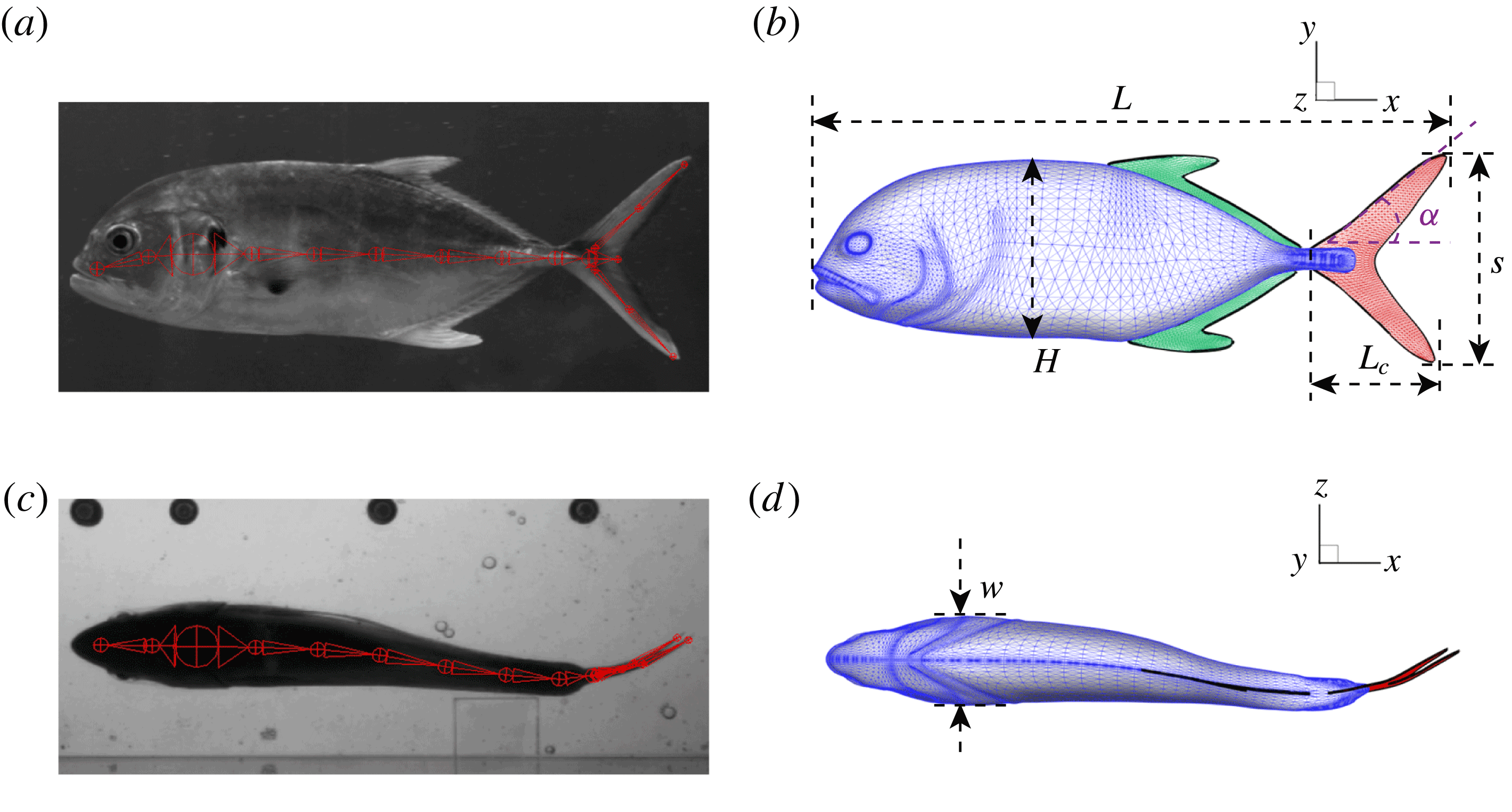
In order to fully understand the body–fin interactions as well as to identify the hydrodynamic role of the body and the fins in fish swimming, three computational models, a full body–fin model (M1) including the dorsal fin and the anal fin as shown in figure 1(b), a body–caudal-fin model (M2) and a caudal fin-only model (M3, highlighted in red), are built for the flow simulation. The models use the same undulatory motion documented in figure 2. Force production and power consumption of the body and the fins are compared among these three models to assess the corresponding hydrodynamic performance. Flow mechanisms are studied by analysing the vorticity fields and the surface force distribution in detail. The effects of fish size and undulatory frequency on the associated findings in body–fin and fin–fin interactions are also examined by varying two key flow parameters, the Strouhal number (
 $St$
) and the Reynolds number (
 $Re$
), respectively.
Snapshots of a Crevalle Jack (Caranx hippos) fish swimming steadily at
 $2L/s$
during one representative tail beat cycle.

The rest of this paper is organized as follows. First, live fish experiments, morphometrics and model reconstruction are presented in § 2. Then, the simulation methodology is presented in § 3. A detailed discussion of the hydrodynamic performance and the vortex structures observed over different computational models and their changes along with key flow parameters (
 $St$
and
 $Re$
) are included in § 4. Finally, conclusions are provided in § 5.
2 Jack fish body–fin model and kinematics
Live fish experiments were conducted by following the same protocol as previous work (Akanyeti et al.
Reference Akanyeti, Thornycroft, Lauder, Yanagitsuru, Peterson and Liao2016). The model of a Crevalle Jack (Caranx hippos) was selected for the computational study. This fish species belongs to the family Carangidae, after which one of the major fish swimming modes, Carangiform locomotion, is named. In the laboratory’s water tunnel, we swam 12 individuals (mean total length
 $L=33.8\pm 1.8~\text{cm}$
) in a recirculating flow tank at speeds ranging from 1 to 4 body lengths per second (
 $L/s$
). Since body kinematics did not change much with speed, we selected one representative swimming speed for an average-sized individual (
 $2.0L/s$
,
 $L=31~\text{cm}$
) for extracting the kinematics of the fish-like locomotion in the current study. The swimming kinematics is recorded with two synchronized high-speed high resolution cameras (ventral and side view) at 500 f.p.s. Six snapshots during a full undulatory cycle in ventral view are shown in figure 2. At the swimming speed studied here, the fish’s pectoral fins and pelvic fins were held against the body throughout swimming and are thus not expected to have a significant effect on the predicted hydrodynamics. As such, only the fish’s trunk (TK), dorsal fin (DF), anal fin (AF) and caudal fin (CF) are considered in the full body–fin model (figure 1
b). TK is modelled as a solid body with surface closed and the fins are modelled as zero-thickness membranes. The surfaces of the model are represented by triangular cells. There are in total
 $2.86\times 10^{4}$
surface meshes (TK:
 $2.27\times 10^{4}$
, DF:
 $1.66\times 10^{3}$
, AF:
 $1.68\times 10^{3}$
, CF:
 $2.56\times 10^{3}$
) used in the model to resolve the complexity of the body and fins.
The key geometric quantities are marked in figure 1(b,d) and measured when the fish body and fins are stretched (see table 1 for the details). Here,
 $L$
represents the total length of the body and is selected as the reference length in our simulations and discussions.
 $H$
and
 $w$
are the body height and body width, respectively.
 $L_{c}$
is the total length of the CF.
 $s$
is its span length and
 $\unicode[STIX]{x1D6FC}$
is the angle between the leading edge of the CF and the horizontal line. All fins areas are measured from the model and are denoted as
 $A_{DF}$
,
 $A_{AF}$
and
 $A_{CF}$
for DF, AF and CF, respectively. The aspect ratio (
 $AR$
) of the CF is calculated as
 $AR=s^{2}/A_{CF}$
.
Geometric quantities of the Crevalle Jack fish model. (All the quantities in length scale and area scale are normalized by
 $L$
and
 $L^{2}$
, respectively.)

The method used to reconstruct the Crevalle Jack body–fin kinematics is the same as that used by Liu et al. (Reference Liu, Ren, Zhu, Bart-Smith and Dong2015) and Fish et al. (Reference Fish, Schreiber, Moored, Liu, Dong and Bart-Smith2016), and is developed from the method employed by Koehler et al. (Reference Koehler, Liang, Gaston, Wan and Dong2012) for tracking the kinematics of insect flights. For completeness, we briefly summarize it as follows. We bound the fish body and fins with a series of virtual skeletons, which were connected one after another and can be rotated about their joints with three degree of freedom (figure 1 a,c). At each time step, we adjust the rotating angles of those skeletons to match our models with the high-speed videos from two orthogonal views. The accuracy of this reconstruction method has been evaluated by comparing the positions of the fish body and fins between the model and the high-speed images. The error was found to be less than 3 %.
The reconstructed body and fin undulatory kinematics of fish model is shown in figure 3. The midline profile (figure 3
a) is similar to that of a carangiform swimmer (Lauder & Tytell Reference Lauder and Tytell2006), in which the anterior half of the body has much smaller oscillating amplitude compared with the posterior tail region. The wavelength (
 $\unicode[STIX]{x1D706}$
) measured from the midline profile is approximately
 $1.05L$
, which is in the range of
 $0.89\sim 1.1L$
observed in most carangiform swimmers (Videler & Wardle Reference Videler and Wardle1991). It is slightly lower than that of a thunniform swimmer (
 $1.16\sim 1.21L$
in yellowfin tuna reported by Dewar & Graham (Reference Dewar and Graham1994)).
(a) Midlines of the Crevalle Jack fish model during undulatory motion. (b) Posterior view of the three-dimensional movement of the model when caudal fin moves from right to left (
 $0\leqslant t/T\leqslant 0.5$
). (c) Movement of the model when caudal fin moves from left to right (
 $0.5<t/T\leqslant 1$
). The red and blue dashed lines above the top and below the bottom of the tail are the trajectories of the upper and the lower tip of the caudal fin, respectively, during a full cycle. The heat map superimposed on the caudal fin shows the lateral amplitude of the caudal fin in the fish frame of reference (
 $z_{c}$
is the position of the midplane when fish body is stretched).

Flapping of the CF exhibits a dorsoventral asymmetry. The 3-D shapes of the fish model during leftward flapping and rightward flapping of the CF are shown in figures 3(b) and 3(c), respectively. The amplitude of the upper tail tip is
 $0.189L$
, which is 13 % higher than that of the lower tip (figure 3
b,c). Also visible is a small phase advance (approximately 4 % of the total period) in the upper tip with respect to the lower tail tip. These kinematic features could cause the dorsoventral asymmetry of the thrust production between the upper and the lower lobe of CF.
In addition, the undulatory motion is not strictly left–right symmetric. This can be seen from the midline shapes in figure 3(a). Also evidence for this asymmetry is that the maximum lateral speed of the upper tip during rightward flapping is approximately 7 % higher than that during leftward flapping of the CF (results not shown here).
In the majority of previous fish swimming studies (Liu & Kawachi Reference Liu and Kawachi1999; Zhu et al. Reference Zhu, Wolfgang, Yue and Triantafyllou2002; Borazjani & Sotiropoulos Reference Borazjani and Sotiropoulos2008; etc.), the undulatory motion was treated as an ideal 2-D kinematic model (a simplified sinusoidal wave) which was based on the midline motion of the fish observed from the dorsal or ventral view. Both the asymmetries of the motion (dorsoventral asymmetry and left–right asymmetry) and their hydrodynamic effects were not considered. However, we do observe the asymmetric features in all jack fish swimming videos. We will describe the hydrodynamic effects of these kinematic asymmetries on the propulsive performance later in this paper.
3 Numerical method and simulations
The 3-D incompressible Navier–Stokes equations are discretized using a cell-centred collocated arrangement of the primitive variables and are solved using a finite-difference-based Cartesian grid immersed-boundary method (Mittal et al. Reference Mittal, Dong, Bozkurttas, Najjar, Vargas and von Loebbecke2008). The equations are integrated in time using the fractional step method. The Navier–Stokes equations are discretized on a Cartesian mesh and boundary conditions on the immersed boundary are imposed through a ghost cell procedure. This method was successfully applied in many simulations of flapping propulsion (Dong et al. Reference Dong, Bozkurttas, Mittal, Madden and Lauder2010; Liu et al. Reference Liu, Ren, Zhu, Bart-Smith and Dong2015; Wan, Dong & Gai Reference Wan, Dong and Gai2015; Liu, Dong & Li Reference Liu, Dong and Li2016). More details about this method can be found in Dong et al. (Reference Dong, Mittal and Najjar2006) and Mittal et al. (Reference Mittal, Dong, Bozkurttas, Najjar, Vargas and von Loebbecke2008) and related validations about this solver can be found in our previous work (Mittal et al. Reference Mittal, Dong, Bozkurttas, Lauder and Madden2006; Dong et al. Reference Dong, Bozkurttas, Mittal, Madden and Lauder2010; Li, Dong & Liu Reference Li, Dong and Liu2015; Wan et al. Reference Wan, Dong and Gai2015).
As shown in figure 4, the simulations are carried out on a non-uniform Cartesian grid. The computational domain size is chosen as
 $12L\times 6L\times 6L$
with
 $384\times 192\times 192$
(approximately 14.2 million) grid points in total. A cuboidal region around the fish model with high-resolution grids (spacing of
 $0.007L$
,
 $0.004L$
and
 $0.0038L$
in the
 $x$
-,
 $y$
- and
 $z$
-directions, respectively) is employed to resolve the near-field vortex structures. At the right-hand boundary (upstream boundary), we provide a constant inflow velocity boundary condition. The left-hand boundary (downstream boundary) is the outflow boundary, allowing the vortices to convect out of this boundary without reflections. The zero-gradient boundary condition is provided at all lateral boundaries. A homogeneous Neumann boundary condition is used for the pressure at all boundaries.
The selection of the current grid set-up is based on extensive tests to ensure that the domain is large enough to achieve accurate results, and grid refinement has been performed to make sure that the simulation results are grid independent. Figure 5 shows the comparison of caudal-fin thrust coefficients of the full body–fin model in three grids. It shows that the difference of both the mean value and the peak value of the thrust coefficient between the medium grid case (adopted in this paper) and the fine grid case is less than 1.8 %. This demonstrates that the hydrodynamic force in the current study is grid independent.
Schematic of the computational mesh and boundary conditions employed in the present simulations.

Comparison of the caudal-fin thrust coefficient of full body–fin model for demonstrating the grid independence of the computed results. The grids employed in the simulations are
 $356\times 144\times 144=7.38\times 10^{6}$
with minimum grid spacing
 $\unicode[STIX]{x1D6E5}_{min}=0.0078$
(for coarse mesh),
 $384\times 192\times 192=14.15\times 10^{6}$
with
 $\unicode[STIX]{x1D6E5}_{min}=0.0038$
(for medium mesh) and
 $412\times 202\times 202=16.81\times 10^{6}$
with
 $\unicode[STIX]{x1D6E5}_{min}=0.0029$
(for fine mesh).

In order to examine the hydrodynamics of the body–fin and fin–fin interactions during undulatory swimming, three computational models were employed to measure the difference between the full body–fin model (M1), the body–caudal-fin model (M2) and the caudal-fin-only model (M3). It is worth noting that the CF kinematics and the flow condition in M3 are the same as those used in M1 and M2. Two key dimensionless parameters, the Strouhal number (
 $St$
) and the Reynolds number (
 $Re$
), are varied to examine the effect of size and frequency on the fish swimming performance. The
 $St$
is defined as
 $St=fA/U$
, where
 $f$
is the flapping frequency;
 $A$
is the averaged peak-to-peak amplitude of the CF and
 $U$
is the swimming speed. The
 $Re$
is defined as
 $Re=UL/\unicode[STIX]{x1D708}$
, where
 $\unicode[STIX]{x1D708}$
is the kinematic viscosity of water.
In the aforementioned laboratory experiments, the measured
 $St$
of the live jack fish swimming is around 0.3 and the
 $Re$
ranges from 110 000 to 457 000. It is very challenging to directly simulate the flow at a
 $Re$
in this range with current computational capabilities. The purpose of the viscous flow simulation is to capture the key features of the wake structures to address the fundamental hydrodynamic mechanisms of fish-like swimming. Previous studies (Buchholz & Smits Reference Buchholz and Smits2006; Bozkurttas et al.
Reference Bozkurttas, Mittal, Dong, Lauder and Madden2009) have shown that the major flow features in flapping propulsion are similar for a changing Reynolds number. Kern & Koumoutsakos (Reference Kern and Koumoutsakos2006) simulated a model fish swimming at
 $Re$
ranging from 2400 to 3900, which is a 5- to 30-fold reduction of that in experimental studies. The wake patterns obtained in their simulations showed strong similarities with the experimental results (Müller et al.
Reference Müller, Smit, Stamhuis and Videler2001). There are also other precedents that reduce the
 $Re$
to the order of
 $10^{3}$
or lower in viscous model simulations of fish swimming (Dong & Lu Reference Dong and Lu2007; Borazjani & Sotiropoulos Reference Borazjani and Sotiropoulos2008, Reference Borazjani and Sotiropoulos2010; Borazjani et al.
Reference Borazjani, Sotiropoulos, Tytell and Lauder2012; Wang, Zhang & He Reference Wang, Zhang and He2012; Liu et al.
Reference Liu, Ren, Zhu, Bart-Smith and Dong2015; Fish et al.
Reference Fish, Schreiber, Moored, Liu, Dong and Bart-Smith2016) with the goal of understanding fundamental physical mechanisms without the requirement of simulating flow features at very large Reynolds numbers, of the order of
 $10^{4}$
or greater. It is worth noting that few studies that employed turbulence models in fish swimming simulations (such as Chang, Zhang & He (Reference Chang, Zhang and He2012) and Bottom II et al. (Reference Bottom, Borazjani, Blevins and Lauder2016)) can be found. In this paper, in order to understand the predominant vortex dynamics, the Reynolds number in the current viscous flow simulation has been reduced to the order of
 $10^{3}$
(see table 2) to meet the requirement of the mesh resolution and computational cost of the simulation of swimming fish models. This is equivalent to a smaller size body performing a slower motion. We have covered a wide range of
 $St$
in our simulations, which is also summarized in table 2. It should be noted that in our simulations we fixed the CF amplitude (mean amplitude of the upper and lower tip) as
 $0.178L$
, according to the measured value from the experiment.
Variations of
 $St$
and
 $Re$
, and the normalized flapping amplitude
 $A/L$
in the current study.

The forces on the fish model’s body and fins are computed through direct integration of the surface pressure and shear, which are projected from the flow variables around the fish body (Mittal et al.
Reference Mittal, Dong, Bozkurttas, Najjar, Vargas and von Loebbecke2008). The thrust force (
 $F_{T}$
, along the swimming direction) is presented as a non-dimensional coefficient (
 $C_{T}$
), which is computed as
 $C_{T}=F_{T}/0.5\unicode[STIX]{x1D70C}U^{2}A_{CF}$
, where
 $U$
is the incoming flow speed and
 $\unicode[STIX]{x1D70C}$
is the fluid density. The total power is defined as the rate of the output work done by the fish model. Its non-dimensional coefficient (
 $C_{P}$
) is defined as,
 $C_{P}=\oint -(\bar{\bar{\unicode[STIX]{x1D748}}}\boldsymbol{\cdot }\boldsymbol{n})\boldsymbol{\cdot }\boldsymbol{V}\,\text{d}s/0.5\unicode[STIX]{x1D70C}U^{3}A_{CF}$
, where
 $\oint$
denotes the integration along the model surface,
 $\bar{\bar{\unicode[STIX]{x1D748}}}$
and
 $\boldsymbol{V}$
represent the stress tensor and the velocity vector of the fluid adjacent to the model surface, respectively, and
 $\boldsymbol{n}$
is the normal vector of each point on the model surface. Note the root region of the CF in both M1 and M2 does not produce force because it is covered by the peduncle of the body model. As such, the force and power produced by the same area in M3 is not included into the calculation of the force coefficients for the comparisons among these three models. The 3-D wake structures are then visualized by the isosurface of the imaginary part of the complex eigenvalue (
 $\unicode[STIX]{x1D706}_{i}$
) derived from the instantaneous velocity gradient tensor, which identifies flow regions where rotation dominates over strain (Mittal & Balachandar Reference Mittal and Balachandar1995; Koehler et al.
Reference Koehler, Wischgoll, Dong and Gaston2011).
4 Results and discussion
In this section, we first present the simulation results of the full body–fin model (M1) at
 $St=0.5$
and
 $Re=2100$
in § 4.1. The comparison among M1, M2 and M3 are shown in §§ 4.2–4.4. Then a parametric study on the effects of the Reynolds number and the Strouhal number is presented in § 4.5.
4.1 Hydrodynamic forces and wake topology of full fish model
In all simulations, five undulatory cycles have been simulated. The hydrodynamic forces of the fish model reach a periodic state after three cycles. The periodic state in M1 is shown in figure 6, where force and power coefficients are plotted as function of time.
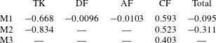
Figure 6(a) shows the time history of the thrust coefficient produced by all four parts, i.e. TK, CF, DF and AF, of the fish model. It indicates that the TK produces drag force (negative
 $\bar{C}_{T}$
), while the CF mainly produces propulsive force during the strokes. Both the TK force and the CF force demonstrate that the force production is slightly different between the leftward flapping and the rightward flapping. This is consistent with the left–right asymmetry of the kinematics discussed in § 2.
Figure 6(b) shows the time history of the power coefficient (
 $\bar{C}_{P}$
) of different body parts. It can be seen that the amplitudes of
 $\bar{C}_{T}$
and
 $\bar{C}_{P}$
of DF and AF are much smaller than those of TK and CF due to their small areas. The cycle-averaged
 $\bar{C}_{T}$
and
 $\bar{C}_{P}$
have also been tabulated in tables 3 and 4, respectively. It is found that the DF and the AF generate a drag force with a small amount of hydrodynamic power consumption. The hydrodynamic benefit of the DF and the AF in the whole body propulsion system will be discussed in the following sections.
(a) Thrust and (b) power coefficients generated by TK, DF, AF and CF of the full body–fin model (M1) during one representative tail beat cycle. The black solid lines in (a) and (b) are total thrust and power, respectively.
 $St=0.5$
,
 $Re=2100$
.

Cycle-averaged thrust coefficient (
 $\bar{C}_{T}$
) generated by the different parts of the fish models (
 $St=0.5$
,
 $Re=2100$
).
Cycle-averaged power coefficient (
 $\bar{C}_{P}$
) generated by the different parts of the fish models (
 $St=0.5$
,
 $Re=2100$
).
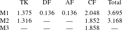
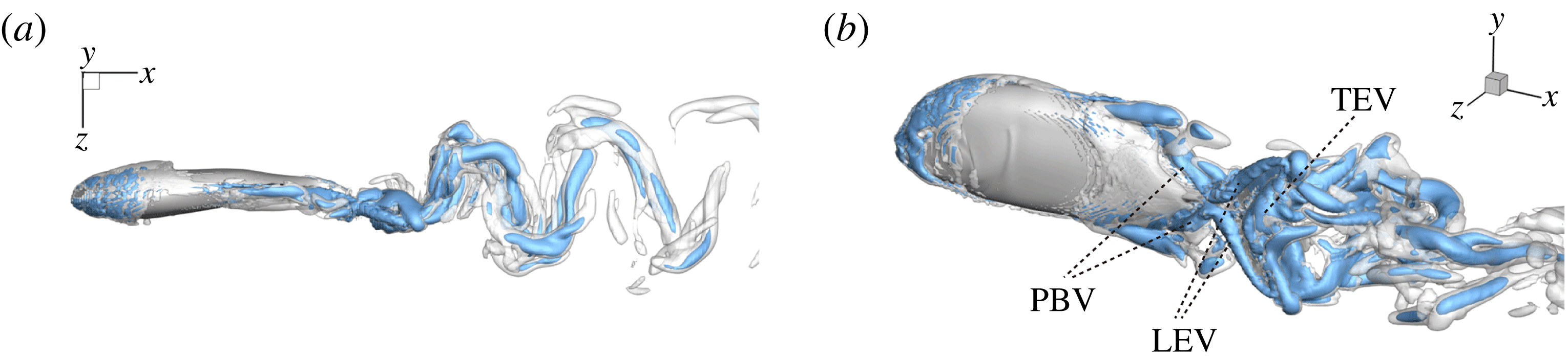
Figure 7 shows the 3-D wake vortex topology of M1 during rightward flapping. From the top view of the flow structures (figure 7
a), two sets of interconnected vortex rings are generated and convect to the downstream. This is consistent with the double row wake structures found by Borazjani & Sotiropoulos (Reference Borazjani and Sotiropoulos2008) at a Strouhal number higher than
 $0.3$
. In addition, many smaller-scale vortices generated from the fish posterior body are found emerged with the vortex rings after interacting with CF. This can be observed in the perspective view of the wake structures (figure 7
b) as well. As indicated in the plot, these small vortices include the trailing-edge vortices (TEVs), the posterior body vortices (PBVs) and the leading-edge vortices (LEVs). In particular, the PBVs, which are generated by the posterior part of the body, will be inevitably captured by the CF, termed the caudal-fin wake capture mechanism in this paper. This will further affect the strength of the LEVs formed around the caudal fin. The consequent change of the propulsive performance will be investigated later.
Three-dimensional wake structures in M1 at
 $t/T=0.67$
from (a) the top view and (b) a perspective view. The wake structures are visualized by the isosurface of
 $\unicode[STIX]{x1D706}_{i}$
.
 $|\unicode[STIX]{x1D706}_{i}|=5.6$
is for the isosurface in white and
 $|\unicode[STIX]{x1D706}_{i}|=11.2$
highlights the vortex core in blue.
4.2 Comparison of body and fin performance in the models
Following the same simulation set-up as in the previous section, the hydrodynamic role of TK, DF and AF in the fish model propulsion is examined by evaluating their performance in M1, M2 and M3, respectively.
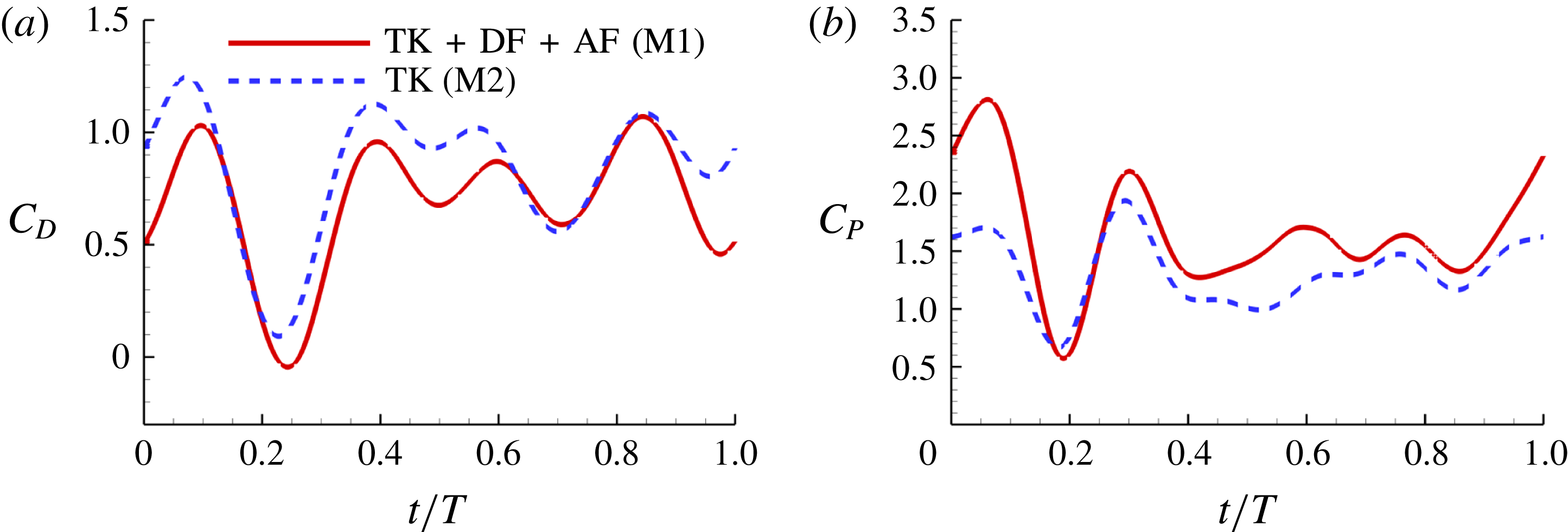
Figure 8(a) shows the comparison of body drag between the M1 model and the M2 model. Table 3 summarizes the cycle-averaged drag coefficients of the fish body, the median fins and the caudal fin in all three computational models, respectively. The total drag coefficient in M1 is 0.668, which is 20 % smaller than that of M2. This indicates a significant body drag reduction due to the appearance of the median fins on the fish body in M1. In the mean time, the thrust produced by the CF in M1 is found to be 13.4 % higher than that produced in M2. From the time history of caudal-fin thrust production in figure 9(a), it is found that the enhancement happens in the mid-strokes.
Figures 8(b) and 9(b) show the comparison of the time history of hydrodynamic power consumption between M1 and M2 by the body and the tail, respectively. Results in table 4 indicate that 16.7 % more total hydrodynamic power is needed in M1 due to the appearance of the median fins. To further understand the propulsive efficiency of both models, the Froude efficiency
 $\unicode[STIX]{x1D702}_{F}$
(Liu, Wassersug & Kawachi Reference Liu, Wassersug and Kawachi1996; Liu, Yu & Tong Reference Liu, Yu and Tong2011a
,Reference Liu, Yu and Tong
b
) is compared between M1 and M2. It is defined by
 $\unicode[STIX]{x1D702}_{F}=\bar{C}_{T}\cdot \tilde{U} /\bar{C}_{P\_T}$
, where
 $\bar{C}_{T}$
is the cycle-averaged CF thrust coefficient,
 $\bar{C}_{P\_T}$
is the cycle-averaged total power coefficient and
 $\tilde{U}$
is the non-dimensional incoming flow speed. It is found that the Froude efficiencies in M1 and M2 are 16 % and 16.5 %, respectively. This indicates that change of the swimming efficiency due to the median fins is only approximately 3 % with remarkable body drag reduction and tail thrust enhancement.
(a) Drag coefficient (
 $C_{D}=-C_{T}$
) and (b) power coefficient (
 $C_{P}$
) of the fish body in M1 (TK, DF and AF together) and M2 (TK only) during one representative tail beat cycle. In both cases,
 $St=0.5$
,
 $Re=2100$
.
(a) Caudal-fin-generated thrust coefficients and (b) caudal-fin power coefficients of M1, M2 and M3 during one representative tail beat cycle. In all cases,
 $St=0.5$
,
 $Re=2100$
.
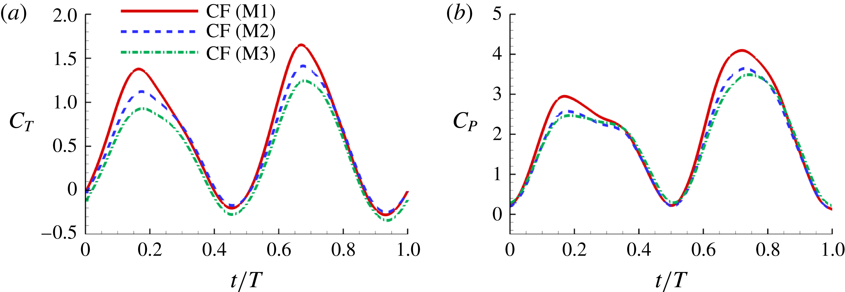
In order to understand the effect of the body–fin interaction on the tail’s propulsive performance, comparison of tail force production and its hydrodynamic power consumption between M2 and M3 are shown in figure 9 and table 3. It is found that the thrust force produced by the caudal fin in M2 is 29.8 % higher than that produced in M3. This suggests that in carangiform swimming the fish body has positive impact on the thrust production of the CF. In addition, the time history of the hydrodynamic power coefficients (
 $C_{P}$
) of CFs in M2 and M3 is shown in figure 9(b). We can see that the CF power consumptions in the both cases are very close during the stroke. From table 4, the cycle-averaged power coefficients are 1.852 and 1.858 in M2 and M3, respectively. This implies that trivial extra hydrodynamic power is needed for the CF’s 29.8 % thrust gain due to the presence of TK.
In summary, both body–fin and fin–fin interactions could result in remarkable hydrodynamic benefits in terms of propulsive force production and body drag reduction. First, the body drag is found alleviated by 20 % comparing the body–median-fin model and the body-only model. Second, the caudal-fin thrust is found a 29.8 % increase by comparing the body–caudal-fin model and the caudal-fin-only model. Third, the caudal-fin thrust production by the full body–fin model is found to be 13.4 % higher than that produced by the body–caudal-fin model.
4.3 Vortex dynamics analysis
In this section, we aim to understand the mechanisms of the above performance enhancement by analysing the flow structures of the three models. Figures 10 and 11 show the comparison of instantaneous wake structures during the leftward flapping and rightward flapping, respectively. Plots associated with M1, M2 and M3 are placed in the left column (labelled a1,b1,c1, see also supplementary movie 2), middle column (a2,b2,c2) and the right column (a3,b3,c3), respectively. The major vortical structures are also labelled in these two figures. The superscripts ‘
 $l$
’ and ‘
 $r$
’ represent the vortices generated during the leftward flapping and rightward flapping, respectively.
4.3.1 Formation of major vortices
In case M1, PBVs are generated periodically by the upper and lower edges of the posterior body. Taking the upper edge as an example, at
 $t/T=0.17$
(figure 10
a1), a fully developed
 $\text{PBV}^{l}$
tube is found attaching to the body. Later on, this vortex tube is separated from the body and moves downstream slightly (figure 10
b1). At the end of the leftward flapping (figure 10
c1), a new vortex tube (
 $\text{PBV}^{r}$
), which has opposite direction compared to the previous
 $\text{PBV}^{l}$
, is formed. The major feature of PBVs in the present study is similar to the body vortices generated by a larvae fish (figure 2 in Li et al. (Reference Li, Müller, van Leeuwen and Liu2016)), which exploits the body vortices to produce thrust. It can also be seen that the strength of the PBVs in M1 case is much stronger than that formed in M2 (figure 10). This would lead large instantaneous pressure difference between the left and right side of the fish body in M1. The comparison of the resulting surface pressure distribution between M1 and M2 will be discussed in a later section.
Three-dimensional wake structures in M1 (a1,b1,c1), M2 (a2,b2,c2) and M3 (a3,b3,c3) at (a)
 $t/T=0.17$
; (b)
 $t/T=0.31$
; (c)
 $t/T=0.46$
. The wake structures are visualized by the isosurface of
 $\unicode[STIX]{x1D706}_{i}$
.
 $|\unicode[STIX]{x1D706}_{i}|=5.6$
is for the isosurface in white and
 $|\unicode[STIX]{x1D706}_{i}|=11.2$
highlights the vortex core in blue. The arrows indicate the directions of the vortex tubes or vortex rings. The CF is flapping leftwards in this figure.

Three-dimensional wake structures in M1 (a1,b1,c1), M2 (a2,b2,c2) and M3 (a3,b3,c3) at (a)
 $t/T=0.58$
; (b)
 $t/T=0.67$
; (c)
 $t/T=0.79$
. The wake structures are visualized by the isosurface of
 $\unicode[STIX]{x1D706}_{i}$
.
 $|\unicode[STIX]{x1D706}_{i}|=5.6$
is for the isosurface in white and
 $|\unicode[STIX]{x1D706}_{i}|=11.2$
highlights the vortex core in blue. The arrows indicate the directions of the vortex tubes or vortex rings. CF is flapping rightwards in this figure.

A recent numerical study by Borazjani & Daghooghi (Reference Borazjani and Daghooghi2013) reported that attached LEVs were formed in caudal fins undergoing fish-like flapping kinematics. Our simulations confirm the existence of LEVs in carangiform swimming. At the early stage of the rightward flapping, for example, at
 $t/T=0.58$
(figure 11
a), rudiments of the LEVs are found to be attached to the leading edges of CF. At (
 $t/T=0.67$
), two obvious LEV tubes are formed (see
 $\text{LEV}^{r}$
in figure 11
b). At this moment, the thrust force reaches a peak value as shown in figure 9(a). This is because of the high pressure difference between the left side and the right side of the CF generated by the LEVs. When the CF flaps rightwards, the LEVs become larger and are about to be shed (figure 11
c). At this moment, the whole left side surface of the CF is covered by the LEVs. At the end of this half-stroke, the LEVs move downstream along with the fin surface and eventually merge with the vortices generated by the trailing edge. This vortex merging forms a big TEV and this TEV sheds from the trailing edge of the CF after the stroke reversal (figure 10
a). This TEV, together with the previous shed TEV, forms a vortex ring and then convects downstream (figure 10
b,c). The latest vortex rings are labelled R1 and R2 in figures 10 and 11, respectively (we do not label R1 in case M1 and M2 in figure 10 as they are blocked by other smaller vortical structures).
4.3.2 Interactions between PBVs and LEVs
As the PBVs move downstream, they will inevitably interact with the aforementioned vortices produced by the caudal fin. For instance, at the middle of rightward flapping in M1 (figure 11
b1), the CF flaps through the
 $\text{PBV}^{l}$
so that the
 $\text{PBV}^{r}$
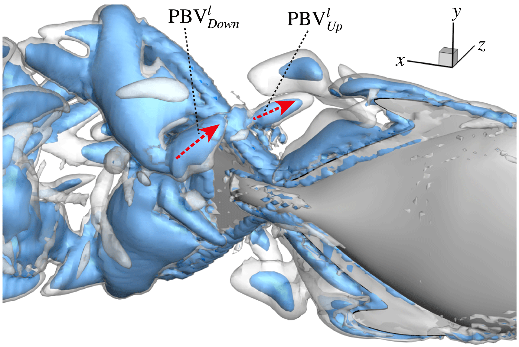
is cut into two parts, the downstream part and the upstream part. We label these two parts in figure 12 (see
 $\text{PBV}_{Down}^{l}$
and
 $\text{PBV}_{Up}^{l}$
), which shows the flow structures from the right-side view at the same moment as figure 11(b1). The downstream part (
 $\text{PBV}_{Down}^{l}$
) is on the right side of the CF and merges with the
 $\text{TEV}^{r}$
. Later on, it will shed from the trailing edge. However, the upstream part (
 $\text{PBV}_{Up}^{l}$
) gets around the leading edge and moves towards the left side. It will be further stretched and elongated as the CF keeps flapping leftwards (figure 11
c1). At
 $t/T=0.79$
(figure 11
c1), we can observe four PBV tubes on the left side of the CF. In the following leftward flapping, these vortex tubes will shed into the wake behind the CF. Similar flow features can be seen in M2 with much weaker PBVs than those observed in M1. This indicates a weaker wake capture between the CF and the PBVs in M2.
 $\text{PBV}^{l}$
is cut into two parts at
 $t/T=0.67$
.
 $\text{PBV}_{Up}^{l}$
and
 $\text{PBV}_{Down}^{l}$
are upstream part and downstream part, respectively. The CF is flapping rightwards.
An obvious feature of this interaction is that the upper and lower PBVs are compressed towards the root region of CF when they propagate downstream after shedding from DF and AF. This is mainly because of the narrowing of the posterior body. Those PBVs will merge with the LEVs near the root region of CF. Similar vortex compression of the PBVs can be found in Zhu et al. (Reference Zhu, Wolfgang, Yue and Triantafyllou2002) (e.g. figure 8 in their paper), in which a potential flow model was used.
In order to better illustrate the compounding vortex interactions near the root region of the CF, we use two different slices (vertical and horizontal) to cut the flow field near this region. Figures 13 and 14 show the contour of
 $\unicode[STIX]{x1D714}_{x}$
and
 $\unicode[STIX]{x1D714}_{y}$
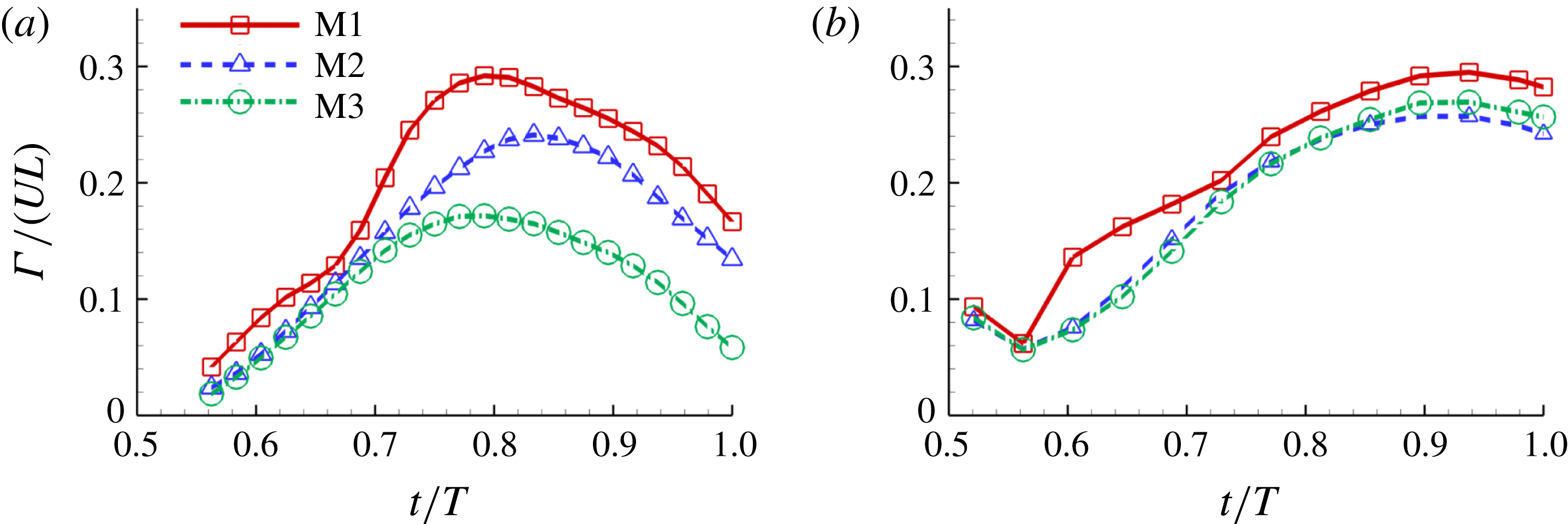
on the two slices, respectively. Comparison of the corresponding circulations is shown in figure 15.
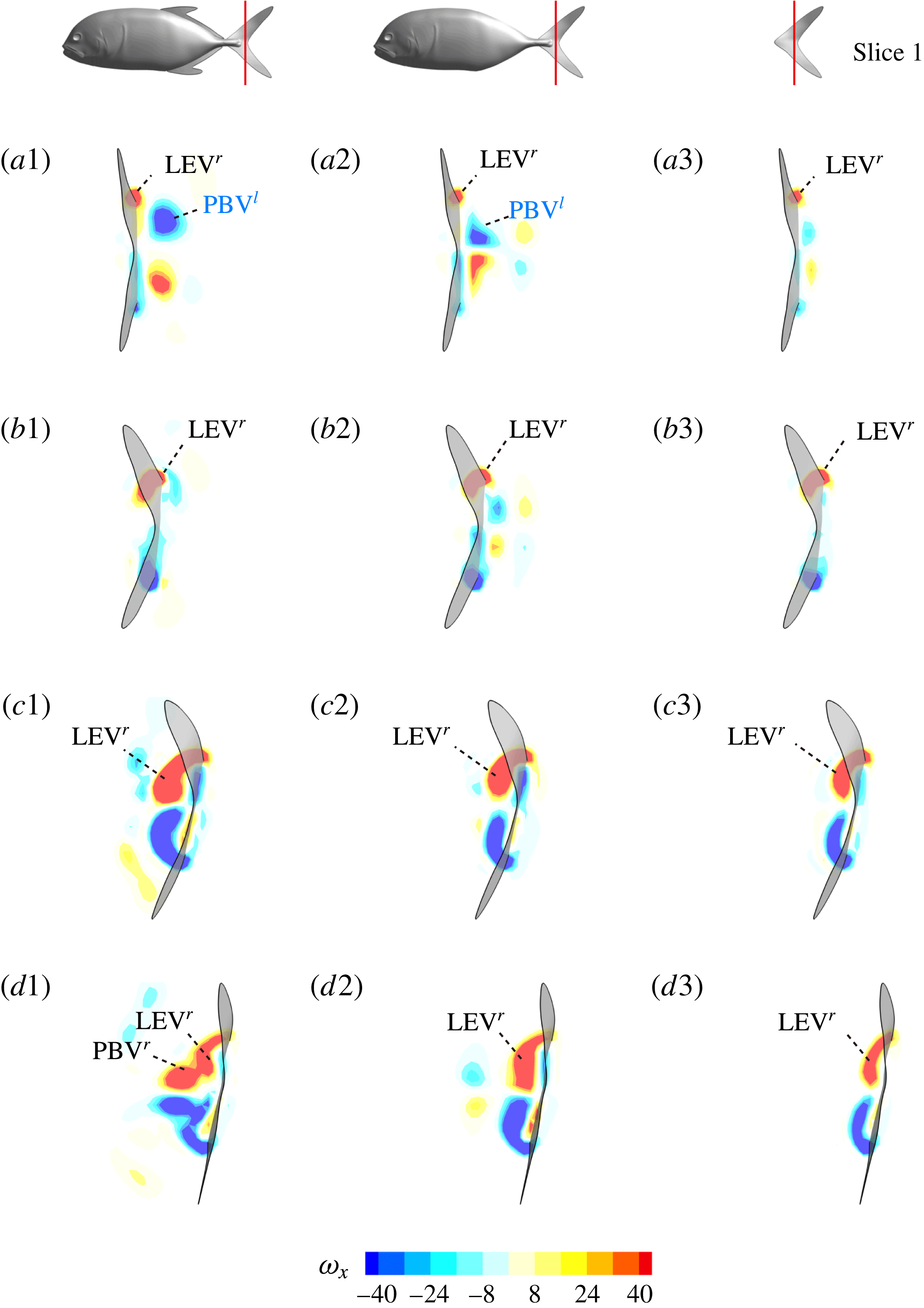
Contour of
 $\unicode[STIX]{x1D714}_{x}$
on a vertical slice (slice 1 whose position is shown by the red lines on the top of this figure) cutting through the flow field of case M1 (a1,b1,c1,d1), case M2 (a2,b2,c2,d2) and case M3 (a3,b3,c3,d3). (a)
 $t/T=0.58$
; (b)
 $t/T=0.67$
; (c)
 $t/T=0.79$
; (d)
 $t/T=0.94$
.
Contour of
 $\unicode[STIX]{x1D714}_{y}$
on a horizontal slice (slice 2 whose position is shown by the red lines on the top of this figure). (a1,b1,c1): model M1; (a2,b2,c2): model M2; (a3,b3,c3): model M3. (a)
 $t/T=0.56$
; (b)
 $t/T=0.625$
; (c)
 $t/T=0.69$
.

Circulation (
 $\unicode[STIX]{x1D6E4}$
) of (a) vorticity
 $\unicode[STIX]{x1D714}_{x}$
on slice 1 and (b) vorticity
 $\unicode[STIX]{x1D714}_{y}$
on slice 2 of the
 $\text{LEV}^{r}$
labelled in figures 13 and 14, respectively. The circulation is normalized by
 $UL$
and only the results during rightward flapping of CF is shown.
Surface pressure of M1 (a1,b1) and M2 (a2,b2) at
 $t/T=0.25$
: (a1,a2) show the left side of fish model from a perspective view; (b1,b2) show the right side from another perspective view. The pressure coefficient is defined as
 $\tilde{p}=(p-p_{\infty })/0.5\unicode[STIX]{x1D70C}U^{2}$
, where
 $p_{\infty }$
is the pressure in the free stream. Red and blue contours mean higher and lower pressure, respectively, relative to
 $p_{\infty }$
. These two colours indicate pushing (red) and suction (blue) forces acting on the body surface, respectively.
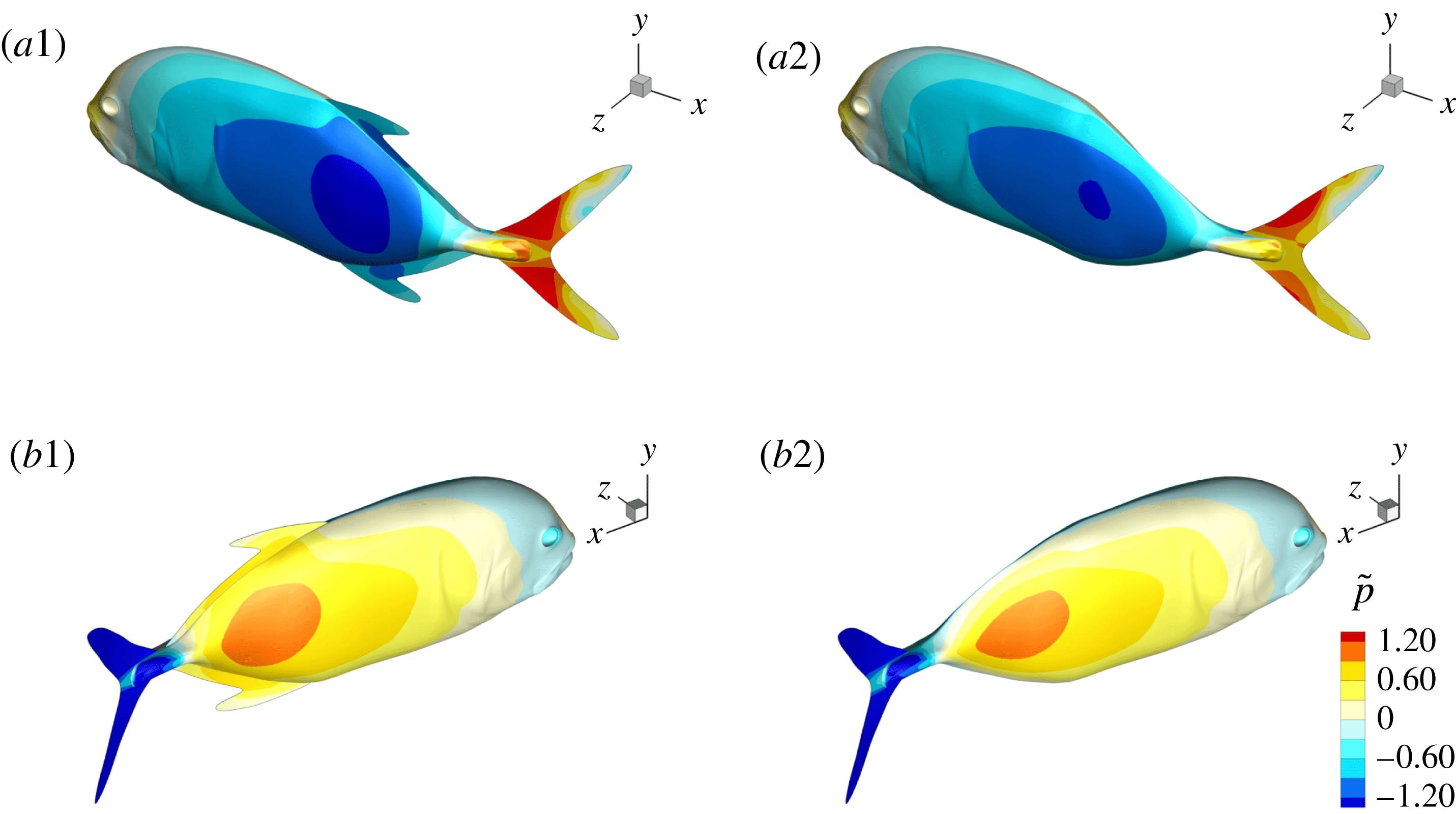
Figure 13 shows four snapshots of the contours of
 $\unicode[STIX]{x1D714}_{x}$
on a vertical slice (slice 1) during rightward flapping for model M1 (a1,b1,c1,d1), M2 (a2,b2,c2,d2) and M3 (a3,b3,c3,d3). In all cases, the strength of the vorticity
 $\unicode[STIX]{x1D714}_{x}$
of
 $\text{LEV}^{r}$
first increases (see figure 13
a–c) and then decreases in the late stage of this stroke (see figure 13
c–d). However, the difference of
 $\unicode[STIX]{x1D714}_{x}$
development between these models is more obvious, which indicates the effect of the body–caudal-fin interaction on the streamwise vorticity near the root region. At the early stage, besides the LEVs, we can also observe two concentrated vortices on the right side of CF in both M1 and M2. These two vortices are the PBVs generated by the previous leftward flapping (see
 $\text{PBV}^{l}$
in figure 13
a1,a2). As discussed in § 4.3.1, after detaching from the body, those PBVs will propagate downstream and soon shed into the wake behind CF, which is the reason that those two PBVs become much weaker at
 $t/T=0.67$
(figure 13
b1,b2). But the newly generated PBVs (
 $\text{PBV}^{r}$
) in the present stroke are also propagating downstream. When they pass the CF root region, they will enhance the LEV by merging into it. This explains the much higher strength of
 $\text{LEV}^{r}$
in M1 compared with that in M3 at
 $t/T=0.79$
(see figure 13
c1,c3). Since the PBVs in M2 are not as strong as those in M1, the strength of LEVs in M2 is in between M1 and M3 (see figure 13
c2). Later on, however, the
 $\text{PBV}^{r}$
will separate with
 $\text{LEV}^{r}$
before the stroke reversal (see figure 13
d1). During the stroke reversal of M1, the
 $\text{LEV}^{r}$
is diminishing, leaving the
 $\text{PBV}^{r}$
on the left side of the tail. And then a new
 $\text{LEV}^{l}$
will be generated, which is like figure 13(a1) but is a left–right reflection. It should be noted that the streamwise vorticity enhancement of LEV is mainly due to the interaction between the LEV and PBV generated by the same stroke (
 $\text{LEV}^{r}$
and
 $\text{PBV}^{r}$
).
The dynamics of the vorticity
 $\unicode[STIX]{x1D714}_{y}$
near the CF root region is also examined. We plot a series of vorticity
 $\unicode[STIX]{x1D714}_{y}$
contours on a horizontal slice (slice 2) shown in figure 14. Vorticity
 $\unicode[STIX]{x1D714}_{y}$
of PBVs in M1 is much stronger than that in M2 by comparing the left column and the right column in this figure. This is consistent with the comparison of the 3-D flow structures between these two models. It should be noted that the PBVs in M1 could maintain their strength after shedding from the posterior body. As a result, a LEV enhancement mechanism whereby the CF captures the vorticity from the upcoming PBVs in case M1 can be found in this figure (see figure 14
a1,b1). However, unlike the enhancement of
 $\unicode[STIX]{x1D714}_{x}$
, the strength increase of
 $\unicode[STIX]{x1D714}_{y}$
is due to the interaction between the LEV generated in this stroke (
 $\text{LEV}^{r}$
) and the PBV generated in the previous stroke (
 $\text{PBV}^{l}$
). In models M2 and M3, the aforementioned interactions are not seen. This is because the
 $\unicode[STIX]{x1D714}_{y}$
of PBVs in M2 is too weak (figure 14
a2–c2) and the CF in M3 experiences a uniform incoming flow (figure 14
a3–c3).
To quantify the circulation of the vortices, we first visualize the vorticity field using contour lines. After each vortex is identified, a closed contour line is generated around this vortex with a specified vorticity level (10 % of the maximum vorticity was chosen in this paper), and then the circulation is computed along this line. Figure 15 shows the comparison of the strength of both
 $\unicode[STIX]{x1D714}_{x}$
(figure 15
a) and
 $\unicode[STIX]{x1D714}_{y}$
(figure 15
b) among the three models during rightward flapping. It is found that the circulations of both vorticities in model M1 are always higher than those in M2 and M3. According to figure 15(a), even at the early stage of the rightward flapping, circulation of
 $\unicode[STIX]{x1D714}_{x}$
in M1 is already stronger than those in M2 and M3. This result explains why the CF thrust in M1 is the highest among all three cases. The circulation of the
 $\unicode[STIX]{x1D714}_{y}$
component of the LEVs in M2 has the similar strength as that in M3 (see figure 15
b), however, the streamwise component in M2 is significantly higher than that in M3. As a result, the CF thrust in M2 is in between those of the other two cases.
4.4 Surface pressure and thrust distribution
In this section, we first briefly introduce the pressure distribution on the body to show how the body drag is reduced by DF and AF, and then focus on the thrust distribution on the caudal fin to explore the thrust enhancement mechanism.
The pressure coefficient is defined as
 $\tilde{p}=(p-p_{\infty })/0.5\unicode[STIX]{x1D70C}U^{2}$
, where
 $p_{\infty }$
is the pressure in the free stream. Figure 16 shows the comparison of pressure distribution on fish surface between M1 and M2 at
 $t/T=0.25$
, at which a big valley of the body drag occurs. According to this figure, the anterior bodies in both cases do not exhibit a big pressure difference between the left and right sides, but we do find a significant pressure difference in the posterior body. This is mainly because of the formation of the PBVs, which is consistent with the findings in Li et al. (Reference Li, Müller, van Leeuwen and Liu2016). The low and high pressure acting on the body surface will result in suction and pushing forces, respectively. Apparently, the pressure difference between two sides in M1 is higher than that in M2. This suggests that a higher forward force component is generated in M1 and as a result, the drag force is reduced.
Distribution of the cycle-averaged thrust (
 $\bar{C}_{T}$
) on the caudal fin. (a) M1, (b) M2 and (c) M3.
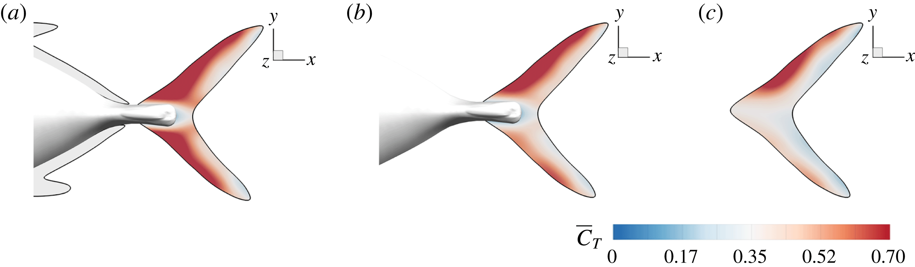
The mean thrust distribution on the caudal-fin surface is also calculated and is shown in figure 17(a–c). This indicates that most of the thrust is generated by the leading-edge region of the caudal fin, which in turn suggests that the LEVs is directly responsible for most of the thrust production. By comparing figure 17(a–c), it is found that the M1 model generates a much higher thrust over a flapping cycle than the other two. This is consistent with the strongest LEVs found in M1 as discussed in previous section.
We also note that the upper half of the CF generates slightly more thrust than the lower half of the fin, especially in M2 and M3 as shown in figure 17(b,c). It is because of the dorsoventral asymmetry of the CF oscillating motion, in which the upper half has a slightly higher amplitude. Unlike M2 and M3, the thrust production in M1 is more symmetric. This is because the height of the AF is approximately 25 % larger than that of DF, which results in a stronger interaction between AF and CF. This improves the thrust production on the lower half of the fin in M1 and results in a more balanced thrust distribution than those in M2 and M3. This even distribution observed in the full body–fin also implies a more stabilized swimming motion by reducing the pitching moment generated by the asymmetry of the force distribution on CF found in M2 and M3.
In summary, our results demonstrate that the interaction between the PBVs and LEVs enhances the strength of the LEVs, thus improving the thrust production of CF.
4.5 Effects of key flow parameters
In this section, we examine the effects of the
 $St$
and
 $Re$
, which are important to the hydrodynamic performance during fish swimming. For a range of each parameter, the body drag and tail-generated thrust among the three models are compared. Only major conclusive results are listed below.
4.5.1 Strouhal number effect
First, we focus on the effect of the Strouhal number,
 $St$
. For this analysis, the
 $Re$
is fixed at 2100. Figure 18(a) shows the variation of the mean body drag coefficient (
 $\bar{C}_{D}$
) with
 $St$
changing from 0.3 to 0.6. It is found that body
 $\bar{C}_{D}$
in M2 does not change too much with
 $St$
, while in M1 it decreases monotonically with an increasing
 $St$
. At a relatively low
 $St$
, the body drag reduction of body–dorsal/anal-fin interaction is not significant at this Reynolds number (
 $Re=2100$
). In particular, at
 $St=0.3$
, the body drag coefficients in M1 and M2 are the same but as
 $St$
increases, the body drag reduction becomes more and more significant.
Figure 18(b) shows the cycle-averaged CF thrust coefficients (
 $\bar{C}_{T}$
) of the three models versus
 $St$
. As
 $St$
increases, the CF thrust coefficients in all models are increasing monotonically. Among these three models, M1 always has the largest CF
 $\bar{C}_{T}$
within the
 $St$
range examined here. And the total thrust enhancement of the fin–fin interaction and body–caudal-fin interaction is always significant by comparing M1 with M3. However, the body–caudal-fin interaction results in more thrust increase (comparison between M2 and M3) than that of fin–fin interaction (comparison between M1 and M2). This result demonstrates that the fin–fin interaction plays an assistant role in the CF thrust enhancement compared with the body–caudal-fin interaction.
(a) Variation of mean body drag coefficients and (b) variation of mean CF thrust coefficients with
 $St$
in three models.
 $Re=2100$
for all cases.

4.5.2 Reynolds number effect
The hydrodynamic performance of the three models with
 $Re$
changing from 500 to 8000 are studied in this section. For this analysis,
 $St$
is fixed at 0.5. The variation of mean body drag coefficients of M1 and M2 with
 $Re$
is shown in figure 19(a). It is found that the body drag is decreasing as
 $Re$
increases, which is mainly because a higher
 $Re$
case has smaller viscous drag. Also visible is that among all
 $Re$
examined in this study, M1 always experiences lower body drag force than M2. And this body drag reduction is more significant at high
 $Re$
cases. According to this trend, a larger benefit due to body–dorsal/anal-fin interaction could be predicted in medium- to large-size fish swimming at a higher
 $Re$
(e.g.
 $Re\geqslant 10^{4}$
).
Figure 19(b) shows the comparison of the mean CF thrust coefficients (
 $\bar{C}_{T}$
) among the three models with a changing
 $Re$
. It is found that for all three models, the CF thrust coefficients are increasing as
 $Re$
increases. Not only the thrust coefficient, the Froude efficiency is also increased as
 $Re$
increases. For instance,
 $\unicode[STIX]{x1D702}_{f}=16\,\%$
in M1 at
 $Re=2100$
while it increases to
 $\unicode[STIX]{x1D702}_{f}=21.7\,\%$
at
 $Re=8000$
(not shown in the figure).
By comparing M1 with M2, we see that the fin–fin interaction leads to an increase of the CF thrust production only at
 $Re>1000$
. Furthermore, this enhancement becomes larger when
 $Re$
is higher. Also found is that, by comparing M2 with M3, the thrust enhancement in M2 reaches a maximum value when
 $Re=500$
among all the cases tested in this study. These results indicate that the thrust enhancement due to body–caudal-fin interaction is more pronounced in relatively low
 $Re$
flows (
 $Re<1000$
), while the fin–fin interaction is more significant in high
 $Re$
flows (
 $Re>4000$
). In addition, the total increase of both fin–fin and body–caudal-fin interactions, as shown in figure 19(b), remains at a constant value when
 $Re>4000$
.
(a) Variation of mean body drag coefficients and (b) variation of mean CF thrust coefficients with
 $Re$
in three models.
 $St=0.5$
for all cases.

5 Conclusions
Numerical simulations have been used to study the hydrodynamics associated with a carangiform swimming model. The body and fin kinematics were reconstructed from experimental measurement using a high-speed photogrammetry system. The focus of the current paper was to examine in detail, the production of forces by the body and fins, the three-dimensional vortex dynamics and body/fin surface force distribution at intermediate Reynolds number flows to understand fish propulsion mechanisms in body–fin and fin–fin interactions.
The simulations revealed that the morphology and motion of fish body and fins (including median fins and the caudal fin) are highly coordinated. Comparisons were made using three different models containing different combination of the fish body and fins to quantitatively measure the performance enhancement and illustrate the associated 3-D vortex dynamics. Simulations indicated that both body–fin and fin–fin interactions could result in remarkable hydrodynamic benefits in terms of propulsive force production and body drag reduction. First, the body drag was alleviated by 20 % comparing the full body–fin model (with median fins) and the body–caudal-fin model (without median fins). Second, the caudal-fin thrust was increased by 29.8 % comparing the body–caudal-fin model and the caudal-fin-only model. Furthermore, the caudal-fin thrust production by the full body–fin model was found to be 13.4 % higher than that produced by the body–caudal-fin model.
Detailed vortex dynamics analysis has shown that the motion of the fish model creates a number of distinct vortex structures including leading-edge vortices and trailing-edge vortices produced by the caudal fin, and posterior body vortices produced by the posterior part of the fish body including the dorsal fin and the anal fin. These vortices convect into the downstream and interact with each other in the wake to create a complex vortex–ring structure. Detailed analyses of the body/fin motion, vortex dynamics and the surface force distribution indicate that during caudal-fin undulatory motion, the formation of a strong and long-lasting attached LEV is responsible for producing most of the thrust. These vortices could be strengthened by capturing the upstream vorticity of the posterior body vortices (caudal-fin wake capture mechanism). Meanwhile, the pressure difference between two sides of the fish body resulting from the PBVs helps with the alleviation of the body drag. The appearance of the median fins further strengthens the PBVs and the caudal-fin wake capture mechanism.
Simulations from a wide range of Strouhal numbers and Reynolds number have shown that the body drag reduction is more significant at high
 $St$
cases, while the enhancement of caudal-fin thrust production due to both the body–caudal-fin and fin–fin interaction is consistently significant at all
 $St$
numbers. The magnitude of body drag reduction due to body–median-fin interaction is more pronounced as Reynolds number increases. Meanwhile, the increase of caudal-fin thrust production is nearly constant when Reynolds number is greater than 4000.
Acknowledgements
This work is supported by National Science Foundation CBET-1313217 and Office of Naval Research (ONR) MURI N00014-14-1-0533. National Institute on Deafness and Other Communication Disorders grant RO1-DC-010809 and National Science Foundation grant IOS 1257150 to J.C.L.
Supplementary movies
Supplementary movies are available at https://doi.org/10.1017/jfm.2017.533.



