1. Introduction
The atomization mechanisms which dictate the primary break-up of a liquid jet are partly defined by the state of the surrounding gas-phase medium (Engelbert, Hardalupas & Whitelaw Reference Engelbert, Hardalupas and Whitelaw1995; Faeth, Hsiang & Wu Reference Faeth, Hsiang and Wu1995; Lasheras & Hopfinger Reference Lasheras and Hopfinger2000; Shavit Reference Shavit2001; Dumouchel Reference Dumouchel2008; Gorokhovski & Herrmann Reference Gorokhovski and Herrmann2008; Shinzo & Umemura Reference Shinzo and Umemura2010; Herrmann Reference Herrmann2011). In the case where a liquid column of bulk mean velocity
 $U_{l}$
is injected into a gaseous flow with a mean velocity
 $U_{g}\gg U_{l}$
, instabilities that form on the liquid jet surface heavily dictate the atomization processes (Sharp Reference Sharp1984; Lin & Lian Reference Lin and Lian1990; Engelbert et al.
Reference Engelbert, Hardalupas and Whitelaw1995; Lasheras, Villermaux & Hopfinger Reference Lasheras, Villermaux and Hopfinger1998; Lasheras & Hopfinger Reference Lasheras and Hopfinger2000; Lee & Park Reference Lee and Park2002; Varga, Lasheras & Hopfinger Reference Varga, Lasheras and Hopfinger2003). This problem is inherently multiscale, and involves wave instabilities developing on the liquid jet surface (Lasheras & Hopfinger Reference Lasheras and Hopfinger2000), large- and small-scale turbulent structures in the surrounding gas-phase medium, as well as random topologies (from ligaments to droplets) that are naturally polydisperse (Lasheras & Hopfinger Reference Lasheras and Hopfinger2000; Gorokhovski & Herrmann Reference Gorokhovski and Herrmann2008; Shinzo & Umemura Reference Shinzo and Umemura2010, Reference Shinzo and Umemura2011; Herrmann Reference Herrmann2011). Practically, such a problem is ubiquitous in steady flow spray applications, such as in gas turbine sprays and propellant systems. While in many practical combustors the gas-phase medium is at elevated temperature and pressure, the investigation of this canonical problem lends itself to the development of simple phenomenological models that allow for basic physical understanding. The atomization process involves a range of mechanisms which take place, likely simultaneously, particularly Kelvin–Helmholtz instabilities and Rayleigh–Taylor instabilities (Beale & Reitz Reference Beale and Reitz1999; Liu & Reitz Reference Liu and Reitz2000; Varga et al.
Reference Varga, Lasheras and Hopfinger2003) along with gas-phase mixing. The latter issue has not received sufficient attention in the literature. Models suggested in coaxial airblast atomizers (Lasheras et al.
Reference Lasheras, Villermaux and Hopfinger1998; Lasheras & Hopfinger Reference Lasheras and Hopfinger2000; Varga et al.
Reference Varga, Lasheras and Hopfinger2003) have not been extended to account for randomness in the flow, and general fundamental understanding of the influence of gas-phase turbulence on break-up phenomena is insufficient. Given that the majority of practical coaxial airblast systems can exhibit gas-phase turbulent inflow conditions or highly intermittent flow fields, suggests that the effect of gas-phase turbulence and fluctuations on air-assisted atomization, be it in primary or secondary atomization, warrants further attention.
Much of the work on coaxial airblast atomizers has been extensively reviewed by Lasheras & Hopfinger (Reference Lasheras and Hopfinger2000) and only a brief account is provided here. The reader should also take note that physical arguments made in air-assisted droplet break-up (Hsiang & Faeth Reference Hsiang and Faeth1992; Lee & Reitz Reference Lee and Reitz1993; Hsiang & Faeth Reference Hsiang and Faeth1995; Arcoumanis, Whitelaw & Whitelaw Reference Arcoumanis, Whitelaw and Whitelaw1996; Liu & Reitz Reference Liu and Reitz2000; Lee & Reitz Reference Lee and Reitz2001) are also relevant to liquid jets as stated by Chigier & Reitz (Reference Chigier and Reitz1995). However, for a thorough overview of secondary atomization, the reader is directed to the review paper of Guildenbecher, Lopez-Rivera & Sojka (Reference Guildenbecher, Lopez-Rivera and Sojka2009). Key dimensionless numbers which define the problem are
 $$\begin{eqnarray}\displaystyle & \displaystyle \mathit{We}=\frac{{\it\rho}_{g}(U_{g}-U_{l})^{2}D_{l}}{{\it\sigma}_{l}} & \displaystyle\end{eqnarray}$$
 $$\begin{eqnarray}\displaystyle & \displaystyle \mathit{we}=\frac{{\it\rho}_{g}(u_{g}-U_{l})^{2}D_{l}}{{\it\sigma}_{l}} & \displaystyle\end{eqnarray}$$
 $$\begin{eqnarray}\displaystyle & \displaystyle \mathit{Re}_{l}=\frac{{\it\rho}_{l}U_{l}D_{l}}{{\it\mu}_{l}} & \displaystyle\end{eqnarray}$$
 $$\begin{eqnarray}\displaystyle & \displaystyle A_{gl}=\frac{D^{2}-D_{l}^{2}}{D_{l}^{2}} & \displaystyle\end{eqnarray}$$
 $$\begin{eqnarray}\displaystyle & \displaystyle m=\frac{{\it\rho}_{l}U_{l}}{{\it\rho}_{g}U_{g}A_{gl}}. & \displaystyle\end{eqnarray}$$
 $\mathit{We}$
based on the mean conditions at the exit plane provides a global measure of the effects of inertial to surface tension forces on spray break-up. An alternative definition of the Weber number can be based on the instantaneous velocity
 $u_{g}$
thus defining the instantaneous Weber number (
 $\mathit{we}$
). For turbulent liquid jets, which is not the case in this manuscript, the liquid jet Reynolds number
 $\mathit{Re}_{l}$
defining the turbulent state of the liquid core is important, and finally
 $m$
is the liquid to air mass ratio, which has been shown to be very relevant in defining atomization behaviour (Lasheras et al.
Reference Lasheras, Villermaux and Hopfinger1998). An additional definition of the Weber number to be used in this contribution is the turbulent Weber number (
 $\mathit{We}^{\prime }$
) defined here by (1.6) which utilizes the turbulent component of the velocity as a relevant scale where
 $u^{\prime }$
is the root mean square (r.m.s.) of the velocity fluctuations:
 $$\begin{eqnarray}\mathit{We}^{\prime }=\frac{{\it\rho}_{g}u^{\prime 2}D_{l}}{{\it\sigma}_{l}}.\end{eqnarray}$$
Depending on the magnitude of the dimensionless scales, a different range of instabilities will form on the liquid jet surface and this problem has been investigated in detail by others as reviewed in Faeth et al. (Reference Faeth, Hsiang and Wu1995), Lasheras & Hopfinger (Reference Lasheras and Hopfinger2000) and Dumouchel (Reference Dumouchel2008). One of the more complete investigations on coaxial airblast atomizers was performed by Engelbert et al. (Reference Engelbert, Hardalupas and Whitelaw1995) providing a full map of droplet size and velocity data in the downstream region. In the nearfield region, primary break-up frequencies as well as overall ‘cluster’ velocities were determined and correlated with the exit Weber number (Engelbert et al.
Reference Engelbert, Hardalupas and Whitelaw1995) showing the importance of the
 $\mathit{We}$
scaling in such flows. More recent work has shown that the primary instability on the liquid jet surface can be related to the vorticity layer thickness that develops around the jet, inside the nozzle
 ${\it\delta}_{g}$
(Raynal Reference Raynal1997). Use of this concept led to the development of a model which relates the ultimate Sauter mean diameter (SMD) of droplets after the break-up process to the most amplified Rayleigh–Taylor wavelength which develops after the primary instability on a liquid column (Varga et al.
Reference Varga, Lasheras and Hopfinger2003). Varga et al. (Reference Varga, Lasheras and Hopfinger2003) found that regardless of the exit mean velocity, the SMD can be related to the Rayleigh–Taylor wavelength through a constant, which was generally tested over mean Weber numbers in the range
 $37<\mathit{We}<437$
. Work by the same group led to a simple break-up length model which uses the momentum flux ratio
 $M={\it\rho}_{g}U_{g}^{2}/{\it\rho}_{l}U_{l}^{2}$
in determining the break-up length, effectively confirming the importance of turbulent entrainment (Lasheras et al.
Reference Lasheras, Villermaux and Hopfinger1998). The consistency in the break-up model results was promising, although not quantitatively confirmed in the paper. Further work was conducted by Liu et al. (Reference Liu, Li, Gong, Cao, Xu, Chen, Wang, Yu, Wang and Yu2006) and ultimately led to a quasi-universal empirical model that could estimate the SMD based on a number of initial conditions. The results showed good agreement with others but a rigorous physical interpretation was not made. More recent work by Kourmatzis, Pham & Masri (Reference Kourmatzis, Pham and Masri2013) has examined an air-assisted atomizer geometry and applied imaging techniques showing that the existence of particular non-spherical shapes in the flow trend with the exit Weber number
 $\mathit{We}$
.
Multiple studies have repeatedly investigated coaxial airblast atomizers (Nukiyama & Tanasawa Reference Nukiyama and Tanasawa1939; Rizkalla & Lefebvre Reference Rizkalla and Lefebvre1975; Lorenzetto & Lefebvre Reference Lorenzetto and Lefebvre1977; Engelbert et al. Reference Engelbert, Hardalupas and Whitelaw1995; Lasheras et al. Reference Lasheras, Villermaux and Hopfinger1998; Villermaux Reference Villermaux1998; Lasheras & Hopfinger Reference Lasheras and Hopfinger2000; Varga et al. Reference Varga, Lasheras and Hopfinger2003; Liu et al. Reference Liu, Li, Gong, Cao, Xu, Chen, Wang, Yu, Wang and Yu2006; Tamaki, Myojin & Yamaji Reference Tamaki, Myojin and Yamaji2011) and have suggested a wide range of models to describe the process. However, the influence of gas-phase turbulence on primary and secondary atomization, and thus the relevance of existing models in highly turbulent environments, requires further attention. In primary atomization, using two-point laser Doppler anemometry (LDA), Shavit (Reference Shavit2001) examined the effect of a liquid jet undergoing break up on the generation of turbulence in the gas phase. However, the results were limited to only a small selection of turbulence intensities, and droplet size measurements were unavailable. Kourmatzis & Masri (Reference Kourmatzis and Masri2014) recently investigated the effects of velocity fluctuations on the atomization of a liquid jet by fixing the mean velocity to a particular value and varying the turbulence intensity, in a similar approach to Shavit (Reference Shavit2001), however under Rayleigh break-up conditions only. This allowed for an isolated understanding of primary break-up, with no secondary atomization. The results showed a very significant effect of gas-phase fluctuations on the primary break-up morphology and a clear dependence of the deformation of droplets on a turbulent Weber number. However, as stated above, the experiments were limited to a weak Rayleigh regime, and measurements were restricted to qualitative information on the break-up structure and droplet deformation data only.
As stated by Chigier & Reitz (Reference Chigier and Reitz1995), delineations between break-up regimes of liquid jets and droplets in air assisted scenarios follow generally comparable trends so it is likely that information with regards to the effects of gas-phase turbulence on secondary atomization will be partly applicable to primary atomization. The effect of gas-phase turbulence on secondary atomization was examined first by Kolmogorov (Reference Kolmogorov1949) showing that for high gaseous Reynolds numbers where fragments of size
 $D_{B}$
satisfy
 $D_{B}\gg {\it\eta}({\it\nu}_{l}/{\it\nu}_{g})^{3/4}$
where
 ${\it\eta}$
is the Kolmogorov scale, then turbulent ‘resonant’ atomization can be exhibited. Hinze (Reference Hinze1955) and Sevik & Park (Reference Sevik and Park1973) revisited the problem and determined a critical turbulent Weber number where the velocity scale was taken as the square of velocity differences across a droplet surface. In general, it is now known that in highly turbulent flows, a critical turbulent Weber number which can lead to a droplet size reduction is far lower than the traditional Weber number leading to break-up (Sevik & Park Reference Sevik and Park1973). Work by Lasheras et al. (Reference Lasheras, Villermaux and Hopfinger1998) examined the effects of turbulence in the far downstream region where resonant break-up can supersede shear atomization of droplets. However, the effect of turbulent fluctuations on instability generation and subsequent droplet size formation were not examined systematically.
In this contribution, a novel experiment is presented to investigate the effects of shear-driven gas-phase turbulence on the primary atomization and break up morphology of non-turbulent liquid jets. A wide range of mean Weber numbers from
 $4.2<\mathit{We}<51.6$
have been examined where for each mean the axial gas-phase turbulence intensity is varied in multiple increments. This results in instantaneous Weber numbers (
 $\mathit{we}$
) that have been measured to vary from approximately 0.4 to
 ${\sim}170$
as deduced from LDA data, and described further in § 3. The experiment forms a platform for the re-examination and expansion of phenomenological models of primary atomization to statistically account for randomness in the flow. The paper is organized as follows: first, the experimental system including the diagnostic and image processing techniques employed are described along with associated errors and uncertainties. The test conditions used are then outlined followed by a presentation of the results which begins with a qualitative discussion of the morphological characteristics of the primary break-up zone. Discussion then progresses to quantitative analysis of both the primary and secondary break-up zones using microscopic backlit imaging and LDA/phase Doppler anemometry (PDA).
2. Experimental methodology
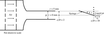
Figure 1 shows a schematic of the experimental set-up. A duct containing laminarizing meshes upstream of the final air ejection nozzle is used to provide an exit flow profile with minimal flow instabilities. The air nozzle in all experiments is fixed to
 $D=10~\text{mm}$
and is approximately 10 jet diameters long. A syringe located within the flow is used to inject an ethanol jet (
 ${\it\rho}_{l}=789~\text{kg}~\text{m}^{-3}$
and
 ${\it\sigma}_{l}=0.024~\text{N}~\text{m}^{-1}$
) which subsequently atomizes. The location of the syringe tip as well as the bulk jet velocity are varied to maintain, at the liquid injection point, conditions of constant mean axial velocity (
 $U_{g}$
) but varying levels of local turbulence intensity (
 $u^{\prime }/U_{g}$
). This is done by injecting the liquid jet both within and outside the valid cone of the turbulent air jet as will be described below. The circles in figure 1 indicate example liquid injection locations and the precise methodology will be described upon presentation of figure 2. The syringe which produces a liquid jet with diameter
 $D_{l}$
is inclined at a slight angle to the horizontal (
 ${\it\theta}=30^{\circ }$
) and this is necessary particularly due to hydraulic components attached upstream of the syringe exit (not shown in figure 1). Injecting at an angle reduces the influence of material disturbing the flow close to the jet but can introduce a slight trajectory, where the effect of this is quantified in § 2.1. Note that the geometry employed here is different to a conventional coaxial air blast atomizer and this is necessary in order to achieve the controlled change in local turbulence intensity for a given fixed mean velocity at the liquid injection location.
Schematic of experimental set-up where circles indicate example liquid jet injection locations.
 ${\it\lambda}_{1}$
is the primary instability wavelength.

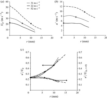
An example of the mean flow (a) and r.m.s. velocity characteristics (b) of the gaseous jets at
 $x/D=10$
for three different bulk air flow cases. Here
 $U_{g}$
is the local mean velocity and
 $u^{\prime }$
the local r.m.s. of velocity fluctuations. The open circles in both figures, indicate three typical experimental cases where the mean flow is fixed but the local r.m.s. changes, these cases are shown in bold in table 1. (c) Plots of
 $u^{\prime }/U_{g}$
(local turbulence intensity) and
 $u^{\prime }/U_{g,r=0\,\text{mm}}$
(turbulent velocity) along with the three cases chosen shown with circles.

To determine the injection locations, it is necessary to map the flow and turbulence fields over a range of bulk jet velocities. The air jets are seeded with water/glycol based droplets of nominal diameter
 $d<1~{\rm\mu}\text{m}$
and LDA measurements are performed on the pure gaseous flow at various axial and radial locations in jets of different bulk velocities. Figure 2(a,b) show radial profiles of mean axial velocity,
 $U_{g}$
and the r.m.s. of the velocity fluctuations
 $u^{\prime }$
for three cases of different centreline mean velocities at
 $x/D=10$
. The measured centreline velocities (
 $U_{g,r=0\,\text{mm}}$
) are noted on figure 2(a). Figure 2(c) presents for each of the three cases, radial profiles of
 $u^{\prime }/U_{g}$
and
 $u^{\prime }/U_{g,r=0\,\text{mm}}$
which are referred to as the local turbulence intensity and turbulent velocity, respectively.
In order to illustrate the experimental procedure adopted, the target of
 $U_{g}=22~\text{m}~\text{s}^{-1}$
(also shown in bold in table 1) is employed here as an example and a similar process is employed for the remaining cases listed in table 1. The circles in figure 2(a) show that for the three bulk velocities shown, a value of
 $U_{g}=22~\text{m}~\text{s}^{-1}$
is obtained when the syringe is located on the centreline for the case of
 $U_{g,r=0\,\text{mm}}=22~\text{m}~\text{s}^{-1}$
(solid curve), at
 $r=6~\text{mm}$
, for the case
 $U_{g,r=0\,\text{mm}}=31~\text{m}~\text{s}^{-1}$
(dotted curve) and at
 $r=10~\text{mm}$
for the case of
 $U_{g,r=0\,\text{mm}}=52~\text{m}~\text{s}^{-1}$
(dashed curve). At these locations, the r.m.s. fluctuations are respectively 5.1, 7.6 and
 $10.1~\text{m}~\text{s}^{-1}$
as shown by the circles in figure 2(b). The resulting turbulent velocities,
 $u^{\prime }/U_{g,r=0\,\text{mm}}$
as well as local turbulence intensities
 $u^{\prime }/U_{g}$
are shown in figure 2(c) as solid and open circles, respectively.
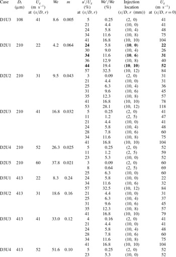
Initial flow conditions (nominal conditions) and dimensionless numbers for all cases examined.

A similar process is followed to locate the syringes for the other selected mean axial velocities of 31, 41, 52 and
 $60~\text{m}~\text{s}^{-1}$
. Table 1 shows the range of cases investigated for each of the three liquid jet diameters (
 $D_{l}$
), the axial and radial locations selected for each case (
 $x/D,r$
), the corresponding local turbulence intensity (
 $u^{\prime }/U_{g}$
) as well as the mean Weber number,
 $We$
, the ratio of turbulent to mean Weber number (
 $\mathit{We}^{\prime }/\mathit{We}$
) and the liquid to air mass ratio,
 $m$
. Also shown in the last column of table 1 are the centreline velocities
 $U_{g,r=0\,\text{mm}}$
corresponding to each case to enable the calculations of the turbulent velocities
 $u^{\prime }/U_{g,r=0\,\text{mm}}$
if needed. The naming of cases listed in table 1 will be used throughout the paper, where D1, D2 and D3 refer to liquid jet diameters
 $D_{l}=108~{\rm\mu}\text{m}$
,
 $D_{l}=210~{\rm\mu}\text{m}$
and
 $D_{l}=413~{\rm\mu}\text{m}$
respectively and velocities U1, U2, U3, U4 and U5, refer to local mean gas-phase velocities
 $U_{g}=22~\text{m}~\text{s}^{-1}$
,
 $U_{g}=31~\text{m}~\text{s}^{-1}$
,
 $U_{g}=41~\text{m}~\text{s}^{-1}$
,
 $U_{g}=52~\text{m}~\text{s}^{-1}$
and
 $U_{g}=60~\text{m}~\text{s}^{-1}$
, respectively.
2.1. Deviation from nominal conditions
In any type of air-assisted spray atomization geometry, after initial injection, the liquid jet will begin to ‘flap’ and radially migrate to different locations of the surrounding expanding air jet. This suggests that slightly downstream of the initial liquid jet injection location, the local flow conditions will change. Nevertheless, in estimates of break-up length (
 $X_{B}$
) and time (
 ${\it\tau}_{B}$
), it is common to use conditions at the injection location as the relevant parameters. In the current experiment, due to the nature of the liquid jet injection technique which is designed to increase the turbulence intensity, the liquid column is injected radially off-centre resulting in injection within a velocity gradient, which is a disadvantage of the technique. This section quantifies the maximum possible deviation from the initial
 $U_{g}$
that the liquid jet experiences, at the break-up length,
 $X_{B}$
.
The trajectory of the liquid can change from outer to inner radial locations leading to an increase in the mean velocity and thus decrease in the turbulence intensity surrounding the liquid. However, this is dependent on the level of liquid jet fluctuation and this effect is measured by observing the maximum and minimum radial displacement of the liquid jet from the initial syringe location up until the break-up length
 $X_{B}$
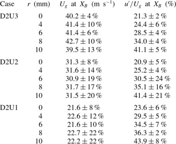
. These measurements are made using the imaging techniques described in §§ 2.2 and 2.3. The break-up length is quantified here from the images as the first location downstream where the main liquid column has formed at least two or more separate liquid packets where further details on the break-up length will be given in § 4. Table 2 shows for a number of cases the average deviation of
 $U_{g}$
and the turbulence intensity from the initial nominal conditions. For a typical case (D2U3) the deviation in
 $U_{g}$
at
 $X_{B}$
from the nominal
 $U_{g}$
value tabulated in table 1 ranges from 4 % at the centreline (
 $r=0~\text{mm}$
) to 13 % at
 $r=10~\text{mm}$
. Clearly, when the liquid jet is injected further off-centre, the local velocity at
 $X_{B}$
will deviate more from the value of
 $U_{g}$
at the initial axial location of liquid injection. However, as will be seen throughout the paper, appropriate physical scalings can be used to describe all results using initial conditions without any corrections. This is substantiated by comparing the radial migration from different liquid jet diameters, which is significantly different. For syringe case D1 for example, the maximum deviation in
 $U_{g}$
at
 $X_{B}$
does not exceed 5 %, in comparison with D2U3 and D2U1 where the deviations are significantly larger as may be seen in table 2. However, all liquid jet diameter scalings collapse based on definitions according to the initial conditions, therefore suggesting that different shear gradients across liquid jets do not supersede the impact of the local turbulence intensity at the jet injection location.
Initial flow conditions (nominal conditions) as well as maximum and minimum deviations from nominal conditions at the break-up length
 $X_{B}$
for selected cases. All cases shown above are for
 $D_{l}=210~{\rm\mu}\text{m}$
.

2.2. Diagnostics
A 2D commercial LDA/PDA system (TSI Model FSA
 $3500/4000$
) has been used both for characterization of the wind tunnel velocities in the ‘
 $X$
’ and ‘
 $r$
’ directions, and also for downstream spray characteristics. The receiver was operated in a
 $45^{\circ }$
forward scattering configuration where more details on the uncertainties of the system are given elsewhere (Gounder, Kourmatzis & Masri Reference Gounder, Kourmatzis and Masri2012).
High-speed imaging is achieved using a backlit microscopic imaging system. This consists of a Nd–YAG diode stack laser (Edgewave) operated at 532 nm and 5 kHz with a nominal power of
 $2~\text{mJ}/\text{pulse}$
as a source of illumination. Two glass diffusing optics are utilized to remove coherence from the beam. The detection system consists of a high-speed CMOS LaVISION camera with a QM-100 long-distance microscope lens. In this experiment the lens was set with a
 $4~\text{mm}\times 4~\text{mm}$
field of view at a pixel resolution of
 $1024\times 1024$
.
Sufficient images were collected for each case by ensuring that multiple integral timescales of the turbulent flow-field were sampled. This is confirmed through computation of the longest integral time scale of the flow, estimated using
 $$\begin{eqnarray}{\it\Lambda}=0.65Rh_{f}\end{eqnarray}$$
where
 $$\begin{eqnarray}\displaystyle & Rh_{f}=0.085X & \displaystyle\end{eqnarray}$$
 $$\begin{eqnarray}\displaystyle & \displaystyle {\it\tau}=\frac{{\it\Lambda}}{u^{\prime }} & \displaystyle\end{eqnarray}$$
 $Rh_{f}$
is the half-radius and
 ${\it\Lambda}$
is the integral length scale (Antonia & Bilger Reference Antonia and Bilger1973). While this is a reasonable estimate at
 $x/D=10$
, the situation is different at
 $x/D=2$
, as the turbulence is under-developed and within the valid cone and therefore a turbulent pipe flow assumption is made as an approximation such that
 ${\it\Lambda}\sim 0.07D$
. By collecting 1000 images per case, the largest integral timescale
 ${\it\tau}$
from all cases, being of the order of
 ${\it\tau}=1.2~\text{ms}$
, is sampled 83 times which is sufficient. These timescales will be quantified for all cases in § 4.1, and it is also confirmed that multiple break-up events are captured given that in § 4.1 it is confirmed that the break-up time is of the same order as the integral timescales.
2.3. Image processing and uncertainties
A detailed calibration technique has been employed here in order to account for defocusing effects when sizing liquid objects and to also make an appropriate choice of background threshold for image binarization. The methodology along with its associated uncertainties is fully described in the appendix of Kourmatzis, Pham & Masri (Reference Kourmatzis, Pham and Masri2014). Using the images, the break-up length is also determined, and this is done by manually observing the first downstream location where more than one object is detected in the image. Given that the images are small scale, this results in a reasonable degree of accuracy which is equal to
 $1/4$
of the field of view, or
 $\pm 1~\text{mm}$
.
In addition to the statistical classification of droplets (spherical objects), statistics are also computed for non-spherical objects as has also been done in the work by Ghaemi, Rahimi & Nobes (Reference Ghaemi, Rahimi and Nobes2009) and Ju, Shrimpton & Hearn (Reference Ju, Shrimpton and Hearn2012). The major axis of these objects will be referred to as
 $D_{max}$
, the minor axis as
 $D_{min}$
and the aspect ratio as
 $AR$
. Two broad types of objects defined here include long ligaments with
 $D_{max}>D_{l}$
and
 $AR>3$
and spherical objects or droplets with
 $D_{max}<D_{l}$
and
 $AR<2$
. While only surface information is presented, it allows for consistent results as demonstrated elsewhere (Kourmatzis et al.
Reference Kourmatzis, Pham and Masri2013).
Throughout the paper, reference to ‘ligaments’ or ‘spherical objects’ (the latter being synonymous to droplets) is made according to the definitions provided above. If reference is made to just an ‘object’ then this implies any liquid fragment detected in the field of view (spherical or otherwise).
3. Primary atomization morphology
One of the inherent assumptions made in the literature is that the primary atomization of an air-assisted liquid jet is dictated by the mean velocity and therefore mean exit Weber number, resulting in a particular break-up regime. It is shown in this paper, from measurement of the gas-phase flow field, for a fixed exit mean Weber number (
 $\mathit{We}$
) that the instantaneous Weber number (
 $\mathit{we}$
) can vary such that a liquid jet is randomly exposed to a range of Weber numbers over a particular length of time. Such variation is controlled in the current experiments. This can span the range from a weak Rayleigh break-up regime where the instantaneous Weber number (
 $\mathit{we}$
) is typically less than 12, to the liquid jet forming a bag-like structure as in secondary atomization, followed by shear break-up at
 $\mathit{we}\gtrsim 80$
when using the same physical arguments as in droplet break-up. As stated in the introduction, differentiation between break-up regimes in air-assisted liquid jet break-up can be roughly categorized following the same approach as with droplets.
3.1. Weber number distribution
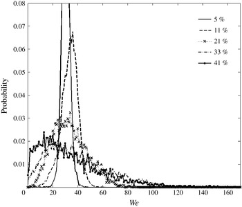
Figure 3 shows an example set of instantaneous Weber number probability distributions calculated from (1.2). This is done here for case D3U3 for a range of turbulence intensities using the measured gas-phase velocity data and assuming here that
 $U_{l}\ll U_{g}$
and
 $D_{l}=413~{\rm\mu}\text{m}$
. The instantaneous Weber number (
 $\mathit{we}$
) is therefore calculated using the time series of velocity. At a turbulence intensity level of 5 %,
 $\mathit{we}$
ranges from approximately 20 to 40 resulting in bag and multimode break-up regimes being possible. At 11 %, the
 $\mathit{we}$
number spans the range 10–50 so the regimes range from a weak Rayleigh or dripping regime to a multimode regime, with the same holding for 21 %. Past a turbulence intensity of 21 %, the
 $\mathit{we}$
range is much broader suggesting that up to four regimes are possible, confirming how an increase in turbulence intensity can substantially affect the break-up process.
Instantaneous Weber number (
 $\mathit{we}$
) probability distributions for case D3U3 (
 $\mathit{We}=33$
,
 $U_{g}=41~\text{m}~\text{s}^{-1}$
,
 $D_{l}=413~{\rm\mu}\text{m}$
) for a variety of turbulence intensities (
 $u^{\prime }/U_{g}\,\%$
).

Of importance is to note that an increase in local turbulence intensity will not just increase the instantaneous Weber numbers but it will also increase the range of Weber numbers about the mean. Therefore, the liquid jet can be exposed from very low-energy break-up to shear type break-up within few break-up timescales. The inertia of the liquid jet can also lead to a memory effect, such that when it is exposed instantaneously to a high and then low velocity, instabilities which developed on the jet surface due to one regime have yet to dissipate, and can interact with another regime. As will be seen in § 4 for the range of cases investigated, the turbulent integral timescale
 ${\it\tau}$
is generally smaller than the break-up time for these jets
 ${\it\tau}_{B}$
suggesting that energy from the surrounding flow-field can indeed be transferred to the liquid jet within a break-up timescale.
3.2. The qualitative effect of turbulence intensity and mean conditions
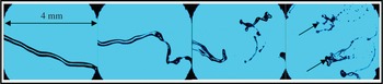
Figure 4 shows typical instantaneous snapshots of the primary break-up zone for case D2U2 for turbulence intensities from 3, 25, 35 and 41 % from left to right with a threshold being applied for purposes of clarity. What is clear from the images is that for a particular mean velocity, a wide range of regimes can be found at the vicinity of the break-up length, which will be quantified later in the paper. For the lowest turbulence intensity case a primary instability is clear, and the jet has yet to break into fragments. For the highest turbulence intensity case, a wider range of break-up regimes is covered and small ‘kinks’ in the liquid jet are commonly observed. These kinks, marked with arrows in figure 4, are generally observable on ligaments which have shed off of the main jet. Given that these ligaments should accelerate, these kinks are consistent with observations of Rayleigh–Taylor instabilities made by others (Lasheras & Hopfinger Reference Lasheras and Hopfinger2000).
Effect of turbulence intensity (3, 25, 35 and 41 % from left to right) on primary break-up morphology for case D2U2 (
 $D_{l}=210~{\rm\mu}\text{m}$
and
 $U_{g}=31~\text{m}~\text{s}^{-1}$
) at
 $X/D_{l}=14$
.

Figure 5 shows typical snapshots of the break-up morphology at a fixed turbulence intensity of 21 %, with an increase in the mean velocity from 22 to
 $60~\text{m}~\text{s}^{-1}$
(D2U1 to D2U5) leading to a decrease in the break-up length, as expected. In addition, kinks are again observable on ligaments ejected from the main liquid column. The overall break-up morphology is therefore similar to what was observed in figure 4 which showed the effects of increasing
 $u^{\prime }$
. However, at a fixed turbulence intensity, the overall deviation of the break-up regimes from the nominal regime defined by the mean conditions is kept constant. Therefore, direct comparison between cases with fixed turbulence intensity reveals only the effect of the overall shear force that exists at the liquid–air interface which leads to the generation of instabilities. When turbulence intensity increases, randomness is added to the break-up structure, and the effects of such randomness will be further explored in this paper.
Effect of mean velocity on primary break-up morphology for 21 % turbulence intensity for cases D2U1 (
 $D_{l}=210~{\rm\mu}\text{m}$
and
 $U_{g}=22~\text{m}~\text{s}^{-1}$
) to D2U5 (
 $D_{l}=210~{\rm\mu}\text{m}$
and
 $U_{g}=60~\text{m}~\text{s}^{-1}$
) of table 1 from left to right at
 $X/D_{l}=14$
.

3.3. Spatial and temporal evolution of the liquid jet
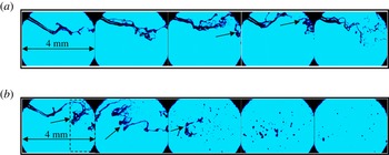
Figure 6(a) shows a typical temporal evolution of the primary break-up zone for case D2U4 which has a fixed turbulence intensity of 23 % at the exit of the syringe. The liquid column is seen to break into a number of liquid shapes including ligaments and droplets. Observing the exit of the liquid column from the syringe, it can be seen that it starts from a well-defined cylinder to a jet shedding ligaments with a highly deformed shape. The greater the turbulence intensity, the more rapid are the changes in the liquid column shape, leading to an instantaneous change in the break-up length. The time elapsed from the first frame to the last frame equates to 1 ms, where the integral timescale
 ${\it\tau}$
for this case corresponds to approximately 0.47 ms. This is
 ${\sim}0.5{\it\tau}_{b}$
where
 ${\it\tau}_{b}$
here is the approximate instantaneous break-up time, although this is revisited in detail in § 4.1. It is evident that the break-up times of these liquid columns occur on similar or longer timescales than the integral scales of the surrounding flow field and therefore interfacial instabilities that are generated on the liquid surface will be heavily influenced by the underlying turbulent flow field. This is examined further in § 4.
Typical temporal evolution with each image separated by
 $200~{\rm\mu}\text{s}$
(a) and typical evolution with downstream distance (b) for case D2U4 (
 $D_{l}=210~{\rm\mu}\text{m}$
and
 $U_{g}=52~\text{m}~\text{s}^{-1}$
) with turbulence intensity equal to 23 %. Dashed box indicates typical zone where liquid core begins to fragment into multiple packets. The middle of the zone, examined from hundreds of images is the location of
 $X_{B}$
.

Figure 6(b) shows a typical evolution of the break-up of the liquid column with downstream position (
 $X$
). The transformation from liquid column, to the generation of instabilities on the jet and finally to droplets is clear through the images. The break-up length of the liquid columns can be determined from images similar to this one as the first location
 $X$
, downstream of the syringe exit plane, where more than one object (spherical or otherwise) is detected. The dashed square shown in figure 6(b) indicates the vicinity of the break-up length, by observing hundreds of images similar to this typical snapshot. The mean break-up length
 $X_{B}$
is therefore a nominal break-up length taken to occur in the middle of this dashed square and this procedure is applied to calculate
 $X_{B}$
as done in § 4.
4. Liquid jet atomization and fragment formation
A particularly interesting theoretical finding in air-assisted primary atomization was that the break-up length can be related solely to the momentum flux ratio of liquid to air
 $M={\it\rho}_{g}U_{g}^{2}/{\it\rho}_{l}U_{l}^{2}$
(Lasheras et al.
Reference Lasheras, Villermaux and Hopfinger1998) although measurements of the break-up length were not made available. This conclusion is strictly only valid for cases where entrainment is the dominant break-up mechanism and where atomization is completely unaffected by surface tension which generally occurs for
 $\mathit{We}>200$
. Here, we measure the primary break-up length directly, and given that r.m.s. velocity measurements (
 $u^{\prime }$
) are also available, the break-up length is quantified as a function of the underlying degree of turbulence and mean conditions. Such a level of detail is not available in the literature.
The relevance of
 $u^{\prime }$
in determining the break-up length is firstly examined by calculating the turbulent Weber number, provided in (1.6). The term inherently accounts for differences in
 $D_{l}$
amongst all of the cases, as well as the measured value of
 $u^{\prime }$
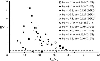
. Figure 7 shows the measured
 $\mathit{We}^{\prime }$
at the injection location plotted versus the break-up length
 $X_{B}$
normalized by the liquid jet diameter
 $D_{l}$
. There are three key variables which seem to control the primary atomization of the liquid jet.
Turbulent Weber number (
 $\mathit{We}^{\prime }$
) versus dimensionless break-up length for all cases of table 1.

The first variable, defined through
 $\mathit{We}^{\prime }$
, is the r.m.s. of the velocity fluctuations. Concentrating on a given case, for example case D2U1, it is clear that there is a trend in the break-up length with
 $\mathit{We}^{\prime }$
, showing the effect of gas-phase turbulent mixing on
 $X_{B}$
. The second variable defining the break-up length is the ratio of mass of liquid to air (
 $m$
), shown in table 1. Going across the plot of figure 7 at a given
 $\mathit{We}^{\prime }$
equal to one for example, it can be seen that the lowest
 $m$
case with a
 $\mathit{We}=8.6$
which corresponds to case D1U3, and the highest
 $m$
case or case D3U1 which has a
 $\mathit{We}=8.3$
show two very different break-up lengths even though their mean Weber numbers are almost identical. This confirms here how
 $\mathit{We}$
is not necessarily as significant as
 $\mathit{We}^{\prime }$
or
 $m$
in determining the break-up length. However, even though the mean
 $\mathit{We}$
number does not show an obvious effect on the break-up length when comparing cases D1U3 to D3U1 it is clear when looking at one particular liquid jet size (for example, all cases of D2). Therefore, a decrease in the break-up length also occurs due to an increase in the mean shear at the liquid–air interface defined by the mean velocity, making mean shear the third governing variable which controls the break-up length. This is particularly true for cases with a very low
 $\mathit{We}^{\prime }$
(those under the dashed line of figure 7), which quite clearly depict the effect of the mean velocity for a fixed liquid jet size. Going from the far right data point under the dashed line (data point from case D2U2) and moving progressively to the left, shows that an increase in the mean velocity (from case D2U2 to D2U3, to D2U4 and D2U5) clearly decreases the break-up length. As will be discussed in § 4.1, the cases underneath the dashed line are those with a very low turbulence intensity, whose break-up lengths are not dictated by
 $u^{\prime }$
, given that for those cases the impact of mean shear is far greater than the impact of fluctuations.
It should be noted that the delineation of various cases with a fuel to air ratio and with the level of
 $u^{\prime }$
agrees directly with the statements of Lasheras et al. (Reference Lasheras, Villermaux and Hopfinger1998) that for shear break-up conditions, the ratio of liquid to air mass, and therefore turbulent entrainment must dictate primary break-up and not the mean Weber number. This is confirmed here over a wide range of turbulence levels. However, it is clear that the primary atomization process is not only governed by
 $u^{\prime }$
,
 $m$
or the mean conditions, but by all three of these variables, suggesting that break-up models must account for them. Clearly, there is a balance where mean interfacial shear supersedes the effect of mixing on primary atomization, and this is now explored further.
4.1. Effect of turbulence on liquid jet atomization
It is apparent from the results of figure 7 that the degree of underlying turbulence, defined by
 $u^{\prime }$
and thus
 $\mathit{We}^{\prime }$
, must partly dictate the atomization process in these flows. For this to be possible an energy transfer must occur from the gas phase to the liquid phase over an appropriate timescale. The break-up time of the liquid column is estimated here from the measured break-up length
 $X_{B}$
as a mean break-up time
 ${\it\tau}_{B}=X_{B}/U_{l}$
where we assume that the main liquid column, prior to atomization travels at a velocity close to
 $U_{l}$
.
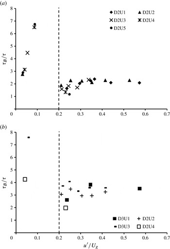
Figure 8(a,b) show the break-up time normalized by the integral timescale
 ${\it\tau}$
for liquid jet cases D2 and D3 (
 $D_{l}=210~{\rm\mu}\text{m}$
and
 $D_{l}=413~{\rm\mu}\text{m}$
) plotted versus the turbulence intensity where
 ${\it\tau}$
is calculated as in § 2.2. There are two regions on both plots showing a significant scatter in the data below a turbulence intensity threshold of 20–25 %. However, for data above this threshold, a reasonably well-defined trend can be observed and this shows agreement with previous work published in Kourmatzis & Masri (Reference Kourmatzis and Masri2014) which examined the effect of turbulence on liquid fragment deformation.
Break-up time (
 ${\it\tau}_{B}$
) normalized by integral timescale (
 ${\it\tau}$
) for cases of table 1 plotted versus turbulence intensity (
 $u^{\prime }/U_{g}$
) where vertical dashed lines indicate approximate zone delineations: (a)
 $D_{l}=210~{\rm\mu}\text{m}$
; (b)
 $D_{l}=413~{\rm\mu}\text{m}$
.

At a nominal turbulence intensity value above 20–25 %,
 ${\it\tau}_{B}/{\it\tau}$
approaches a constant value implying that an increase in the break-up time seems to occur roughly proportionally with an increase in the integral timescale
 ${\it\tau}$
. This is a critical result which indicates that the break-up time or length is directly related to the integral timescale, calculated here from the underlying r.m.s. velocity of the gas-phase fluctuations. This provides further experimental evidence that at sufficient turbulence intensities, the fragmentation of liquid columns is dependent strongly on gas-phase mixing and entrainment and not the mean Weber number, and that the break-up time can be accurately predicted using information about the turbulent eddy statistics.
However, to the far left of the figure 8(a,b), it is clear that the break-up time
 ${\it\tau}_{B}$
can increase to values much higher than the integral timescale, and there is no clear relationship; suggesting that the r.m.s. velocity is not the parameter governing the fragmentation of the jet in regions of low turbulence intensity. This is in direct agreement with previous work by Kourmatzis & Masri (Reference Kourmatzis and Masri2014) which looked at primary atomization in Rayleigh break-up regimes in a different experimental set-up. Here it may be seen that there are clearly mean Weber number dependencies at low turbulence intensities, although further data is required in that region to draw more rigid conclusions.
4.2. Effect of turbulence on liquid fragment formation
It is clear that the turbulent properties of the gas phase are paramount in determining the near-field fragmentation characteristics of the liquid jet. We have experimentally confirmed the theory of Lasheras et al. (Reference Lasheras, Villermaux and Hopfinger1998) that the ratio of liquid to air mass is key in determining the break-up length and have also directly assessed the relevance of the turbulent timescales in dictating the break-up time. A key issue that has not been dealt with in the literature however is what mechanism or range of mechanisms is involved in the final generation of ligaments and droplets in turbulent flows, not only in terms of where the break-up initiates, but also the final size of the objects. In order to isolate the effect of turbulence, and to provide a physical explanation of the generation of liquid fragments, the size of ligament and droplet shapes discussed in § 2.3 is calculated for all cases of table 1. From the images, we can measure the value of the primary instability wavelength or
 ${\it\lambda}_{1}$
, shown schematically in figure 1 and also shown schematically in figure 9( f), and we use this quantity as a datum to delineate between different cases.
Mean ligament lengths normalized by primary instability wavelength (
 $\langle L\rangle /{\it\lambda}_{1}$
) versus downstream location (
 $X/D_{l}$
) for cases of
 $D_{l}=210~{\rm\mu}\text{m}$
where TI is turbulence intensity (
 $u^{\prime }/U_{g}\%$
): (a) D2U1 (
 $D_{l}=210~{\rm\mu}\text{m}$
and
 $U_{g}=22~\text{m}~\text{s}^{-1}$
); (b) D2U2 (
 $D_{l}=210~{\rm\mu}\text{m}$
and
 $U_{g}=31~\text{m}~\text{s}^{-1}$
); (c) D2U3 (
 $D_{l}=210~{\rm\mu}\text{m}$
and
 $U_{g}=41~\text{m}~\text{s}^{-1}$
); (d) D2U4 (
 $D_{l}=210~{\rm\mu}\text{m}$
and
 $U_{g}=52~\text{m}~\text{s}^{-1}$
); (e) D2U5 (
 $D_{l}=210~{\rm\mu}\text{m}$
and
 $U_{g}=60~\text{m}~\text{s}^{-1}$
); ( f) snapshots (
 $3~\text{mm}\times 3~\text{mm}$
) showing initial weak points generated by the primary instability. A sample identification of
 $L$
and
 ${\it\lambda}_{1}$
for D2U4 (
 $D_{l}=210~{\rm\mu}\text{m}$
and
 $U_{g}=52~\text{m}~\text{s}^{-1}$
) at a TI of 4 % is also shown in ( f).

The primary instability wavelength is a measure of the initial interfacial instability that occurs on the liquid jets and according to the findings of Raynal (Reference Raynal1997) is dependent on the density gradient between the liquid jet and the surrounding air as well as the vorticity layer thickness. An expression for estimating
 ${\it\lambda}_{1}$
has been provided in Varga et al. (Reference Varga, Lasheras and Hopfinger2003), assuming a laminar boundary layer developing at the nozzle exit. Given here, that the liquid jet is injected at varying locations along a turbulent expanding jet, a laminar boundary-layer assumption might not be valid. However,
 $$\begin{eqnarray}\displaystyle {\it\lambda}_{1}\propto \left(\frac{{\it\rho}_{l}}{{\it\rho}_{g}}\right)^{1/2}{\it\delta}_{g}\end{eqnarray}$$
should still apply based on the findings of Raynal (Reference Raynal1997). In laminar flows, the vorticity layer thickness
 ${\it\delta}_{g}$
generally scales with
 $1/\mathit{Re}_{g}^{1/2}$
. In a turbulent boundary-layer assumption,
 ${\it\delta}_{g}$
would have to be calculated based on an assumption such as that of
 $$\begin{eqnarray}\displaystyle {\it\delta}_{g}=\frac{C_{2}{\it\Delta}}{\mathit{Re}_{g}^{1/5}}.\end{eqnarray}$$
with a suitable empirical constant
 $C_{2}$
. Here
 ${\it\Delta}$
is the length over which the boundary layer would develop, which would be of the order of multiple jet diameters, where the break-up length
 $X_{B}$
would represent the longest boundary-layer length. These expressions will be utilized in the model calculations of § 6.2. For the purposes of the current analysis however where assumptions are to be avoided,
 ${\it\lambda}_{1}$
is determined directly from the available image data and for cases D2U1–D2U5,
 ${\it\lambda}_{1}$
is equal
 $1000~{\rm\mu}\text{m}$
,
 $700~{\rm\mu}\text{m}$
,
 $700~{\rm\mu}\text{m}$
,
 $492~{\rm\mu}\text{m}$
and
 $400~{\rm\mu}\text{m}$
, respectively, where for cases D3U1–D3U4 and D1U3 it is equal to
 $826~{\rm\mu}\text{m}$
,
 $830~{\rm\mu}\text{m}$
,
 $410~{\rm\mu}\text{m}$
,
 $410~{\rm\mu}\text{m}$
and
 $378~{\rm\mu}\text{m}$
, respectively.
The length of measured fragments (
 $L=D_{max}$
) is presented here with respect to
 ${\it\lambda}_{1}$
which is measured for each case for the lowest turbulence intensity only. This is due to the inability to measure an accurate
 ${\it\lambda}_{1}$
for high turbulence intensity cases given the significant flapping in the liquid jet making
 ${\it\lambda}_{1}$
difficult to extract from the images. It is plausible that different statistical measures of
 ${\it\lambda}_{1}$
can be extracted, however this would require more complex image processing which is beyond the scope of this paper.
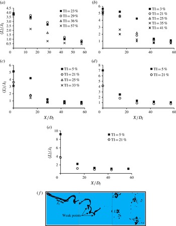
Figure 9 shows the evolution of long ligament mean length (
 $\langle L\rangle$
) (long ligament as defined in § 2.3) versus downstream location. Results are shown for various cases selected from table 1. In figure 9( f) are snapshot images showing how
 ${\it\lambda}_{1}$
and
 $L$
are identified. This mean ligament length is determined from taking the size of individual ligament lengths (
 $L$
) averaged over all images. Concentrating on any of the cases, such as figure 9(b) clearly shows how the turbulence intensity reduces the ligament length at a particular upstream
 $X/D_{l}$
. A striking result is that regardless of the turbulence intensity or mean
 $\mathit{We}$
number, the final mean length of ligaments for all r.m.s. cases converge from an initially different value to a value which is of the order of the primary instability wavelength such that the length
 $\langle L\rangle /{\it\lambda}_{1}\sim 1$
. This is true for all liquid jet sizes, including those not shown here. The results indicate that it is largely the primary instability wavelength that dictates the final size of ligaments prior to their conversion into droplets, where turbulence accelerates this process.
The primary instability can therefore be considered to create weak points along the primary liquid column which initially generates an arbitrary mean ligament size of
 $n{\it\lambda}_{1}$
. The minimum size of a ligament, on average, is obtained where
 $n\sim 1$
but larger values of
 $n$
are possible closer to the initial break-up location. An example of these clearly observable weak points in the primary liquid column is shown in figure 9( f). The data here confirms that those initial weak points lead to the formation of the final ligament lengths defined purely based on a mean primary instability wavelength. Whether or not this holds for other shapes such as spherical droplets, which form the majority of objects in turbulent atomizing sprays must be examined, and this is done in § 4.2.2 after examining ligament formation further.
4.2.1. Ligament convergence distance: mechanism of ligament generation
Given that all long ligaments converge to a final value of
 ${\it\lambda}_{1}$
, it is clear that their final structure is dictated by the primary interfacial instability. However, turbulence intensity leads to an acceleration in the ‘convergence distance’ of the ligaments, or the location downstream (
 $X_{L}$
) where the ligaments reach some constant value of
 $\langle L\rangle /{\it\lambda}_{1}$
, as may be seen through figure 9. This convergence length is calculated here as the distance from the exit plane of the syringe to when the size of ligaments has reached a constant value of
 $\langle L\rangle /{\it\lambda}_{1}=1.5$
. This value of
 $\langle L\rangle /{\it\lambda}_{1}=1.5$
is chosen over
 $\langle L\rangle /{\it\lambda}_{1}=1$
, because some cases do not converge to exactly
 $\langle L\rangle /{\it\lambda}_{1}=1$
and therefore for the sake of consistency and ease of processing, a value slightly larger than
 $\langle L\rangle /{\it\lambda}_{1}=1$
is chosen.
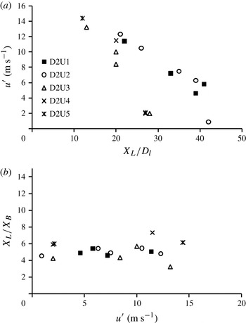
Root mean square of gas-phase velocity fluctuations versus dimensionless ligament length convergence distance (a) and convergence distance normalized by break-up length
 $X_{L}/X_{B}$
versus r.m.s. (b) for
 $D_{l}=210~{\rm\mu}\text{m}$
cases of table 1.

Figure 10(a) shows the r.m.s. of the axial velocity fluctuations
 $u^{\prime }$
plotted versus the dimensionless final convergence length of the long ligaments. The final mean ligament convergence distance
 $X_{L}$
is normalized by the mean break-up length
 $X_{B}$
and plotted versus the axial r.m.s. velocity as shown in figure 10(b). Over the full range of cases, it can be seen that
 $X_{L}/X_{B}\sim 5$
is generally a constant, therefore showing that it is precisely the same mechanism which dictates the length or time that it takes for the liquid column to break and for the ligaments to reach their final state. The break-up length of the liquid column (and for a given
 $U_{l}$
the break-up time of the column) is dictated by the integral length or time scales. Therefore, while the final size of ligaments is well described using
 ${\it\lambda}_{1}$
, the distance to form ligaments is heavily dictated by turbulence. This new result suggests that the same model used to determine the break-up length of a column can also be used to determine the final distance that it takes for ligaments to fully develop. Results such as these should be reproducible in Eulerian models of primary break-up (Desjardins, Moureau & Pitsch Reference Desjardins, Moureau and Pitsch2008; Gorokhovski & Herrmann Reference Gorokhovski and Herrmann2008; Shinzo & Umemura Reference Shinzo and Umemura2010; Herrmann Reference Herrmann2011).
4.2.2. Droplet formation
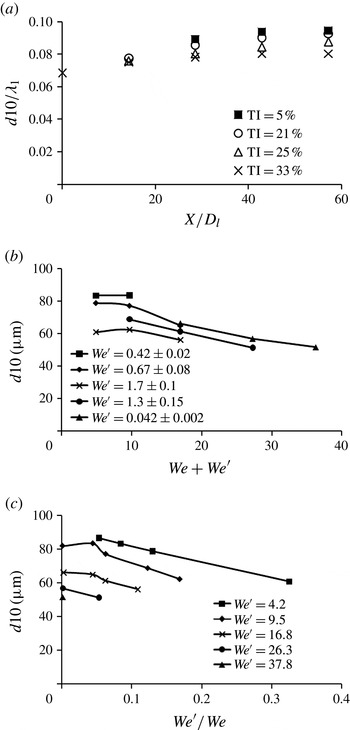
Figure 11(a) shows the evolution of spherical droplets, as described in § 2.3, with downstream location for case D2U3. All other cases of table 1 showed the same trends and are therefore not presented here. A phenomenon that was consistently observed for all cases of table 1 is that while the ligament sizes start from very different values of
 $\langle L\rangle$
they converge to a value of
 $\langle L\rangle /{\it\lambda}_{1}\sim 1$
. In contrast, the mean sizes of spherical droplets, shown in figure 11(a) diverge from a common value as they traverse downstream. This suggests that in these highly turbulent and intermittent flows, as ligaments atomize and become converted into droplets, the final process that leads to the formation of droplets cannot be solely linked to
 ${\it\lambda}_{1}$
, where some evidence of this was also provided in Varga et al. (Reference Varga, Lasheras and Hopfinger2003).
Mean droplet sizes normalized by primary instability wavelength (
 $d10/{\it\lambda}_{1}$
) versus dimensionless downstream location (
 $X/D_{l}$
) for case D2U3 (
 $D_{l}=210~{\rm\mu}\text{m}$
and
 $U_{g}=41~\text{m}~\text{s}^{-1}$
) (a), mean droplet sizes for a variety of cases plotted versus the ‘total’ Weber number (b) and
 $\mathit{We}^{\prime }/\mathit{We}$
(c) at the final downstream location: (a)
 $d10/{\it\lambda}_{1}$
versus (
 $X/D_{l}$
) for case D2U3; (b)
 $d10$
versus
 $\mathit{We}+\mathit{We}^{\prime }$
at
 $X/D_{l}=57$
; (c)
 $d10$
versus
 $\mathit{We}^{\prime }/\mathit{We}$
at
 $X/D_{l}=57$
.

Over all cases examined from table 1, beyond
 $X/D_{l}=20$
, the range of arithmetic spherical object size is of the order of
 $0.06<(d10)/{\it\lambda}_{1}<0.12$
and the SMD is of the order of
 $0.1<d_{SMD}/{\it\lambda}_{1}<0.21$
. The reader should note that an increase in the droplet size with downstream location occurs because ligaments (as defined in § 2.3) atomize and their products are binned by the processing routine as spherical droplets. However, by the end of atomization process there is a clear trend in droplet size with turbulence intensity. While there are clearly differences in the final size of spherical objects at the end of the atomization process, the general order of magnitude of these objects is close to
 $b\sim 0.1{\it\lambda}_{1}$
. This order of magnitude estimate was also observed by Varga et al. (Reference Varga, Lasheras and Hopfinger2003) in ligament thicknesses peeling off of the main liquid jet. Such a boundary-layer stripping model may therefore give an overall estimate of the final droplet size; however, given the divergences amongst cases, such models clearly cannot accurately account for randomness in the flow.
Based on these findings, it is shown here that
 ${\it\lambda}_{1}$
is a key indicator of downstream atomization performance of the majority of the spray volume which is in the form of ligaments. However,
 ${\it\lambda}_{1}$
does not dictate the final formation of spherical droplets which in practical applications, such as in combustion, will dictate the start of flame initiation. Given the importance of this issue, the remainder of this section is dedicated to further analyse the formation of droplets.
Spherical objects are observed to be significantly smaller than
 ${\it\lambda}_{1}$
, and generally decrease in size both with the mean and r.m.s. velocity acting on the liquid jet. This measured decrease in the droplet size is examined here by scaling the size both on the liquid jet mean and turbulent Weber numbers. In addition, by considering a total contribution of mean and dynamic forces on the jet, and assuming
 $U_{l}\ll U_{g}$
, then the total aerodynamic force will be proportional to
 ${\it\rho}_{g}D_{l}^{2}(U_{g}^{2}+u^{\prime 2})$
. This, being counteracted by the restorative surface tension force proportional to
 ${\it\sigma}D_{l}$
, yields a ‘total’ Weber number definition which accounts for both the mean and variance of the flow being equal to
 $\mathit{We}_{total}=({\it\rho}_{g}(U_{g}^{2}+u^{\prime 2})D_{l})/{\it\sigma}_{l}=\mathit{We}+\mathit{We}^{\prime }$
.
Figure 11(b) shows, for curves of constant turbulent Weber number, how the droplet size reduction scales with the total Weber number (
 $\mathit{We}+\mathit{We}^{\prime }$
). Figure 11(b) demonstrates the independent influence of the mean and turbulent components on droplet size for four typical cases. For a given turbulent Weber number, an increase in the overall Weber number, driven in this instance by an increase in the local mean kinetic energy, results in a spray with decreased droplet sizes. This generally occurs above a total
 $\mathit{We}$
equal to 12, corresponding, in secondary atomization, to the bag break-up threshold. At total Weber numbers less than 12, an increase in
 $\mathit{We}^{\prime }$
to values above approximately 0.67 has a substantial effect on the final droplet size. However, this effect reduces as the overall Weber number increases and therefore as the turbulence intensity decreases for a fixed
 $\mathit{We}^{\prime }$
. This is likely due to conventional shear atomization becoming a dominant mechanism at low
 $\mathit{We}^{\prime }$
. Figure 11(c) shows the impact of
 $\mathit{We}^{\prime }$
clearly by scaling the final droplet size to the ratio of
 $\mathit{We}^{\prime }/\mathit{We}$
where at a transition of approximately
 $(\mathit{We}^{\prime }/\mathit{We})=(u^{\prime 2}/U_{g}^{2})\sim 6\,\%$
which corresponds to a turbulence intensity of
 ${\sim}25\,\%$
, a decrease in the droplet size is observed for a fixed mean condition.
Here
 $\mathit{We}^{\prime }$
and
 $\mathit{We}$
are useful global scales given that they can be defined using initial conditions only and do not involve any assumptions. However, figure 11(a), as well as qualitative observation of many images, suggests that the droplets, in general, are not generated directly from the liquid jet, but from liquid ligaments, of length
 ${\it\lambda}_{1}$
. Given that an increase in
 $\mathit{We}^{\prime }/\mathit{We}$
above
 ${\sim}6\,\%$
corresponds to a droplet size reduction suggests that an enhanced degree of atomization could be occurring due to turbulent fluctuations acting on the scale of the liquid ligaments. The data of figure 11(c) is therefore examined further in the context of the traditional turbulent Weber number of Kolmogorov (Reference Kolmogorov1949) (
 $\mathit{We}_{t}$
) given by
 $$\begin{eqnarray}\mathit{We}_{t}=\frac{{\it\rho}_{g}\overline{u_{d}}^{2}D_{B}}{{\it\sigma}_{l}}.\end{eqnarray}$$
In this definition of the turbulent Weber number (
 $\mathit{We}_{t}$
) the relevant velocity scale is taken as the turbulent velocity difference on the scale of the atomizing fragment, assumed here to be a ligament of length
 ${\it\lambda}_{1}$
, and therefore this definition is different to that provided in (1.6). It is confirmed here that
 ${\it\lambda}_{1}\gg {\it\eta}({\it\nu}_{l}/{\it\nu}_{g})^{3/4}$
(a condition discussed in the introduction), however, an assumption must be made about the rate of dissipation of the turbulent kinetic energy
 ${\it\epsilon}$
, and for simplicity, we adopt the assumptions of Sevik & Park (Reference Sevik and Park1973) resulting in
 $$\begin{eqnarray}\overline{u_{d}}^{2}=2({\it\epsilon}D_{B})^{2/3}\end{eqnarray}$$
for the square of the velocity
 $\overline{u_{d}}^{2}$
across the fragment length written in terms of the dissipation
 ${\it\epsilon}$
and shown in
 $$\begin{eqnarray}\overline{u_{d}}^{2}=2({\it\epsilon}{\it\lambda}_{1})^{2/3}=2u^{\prime 2}\left(\frac{{\it\lambda}_{1}}{{\it\Lambda}}\right)^{2/3}\end{eqnarray}$$
in terms of the r.m.s. of the velocity fluctuations.
Determining
 $\mathit{We}_{t}$
from (4.3) for each of the cases of figure 11(c) at
 $\mathit{We}^{\prime }/\mathit{We}=0.06$
yields
 $\mathit{We}_{t}$
values of 0.8, 0.9, 1.7 and 1.4 for cases of
 $\mathit{We}$
equal to 4.2, 9.5, 16.8 and 26.3, respectively. These values of
 $\mathit{We}_{t}$
are in the range of the critical turbulent Weber numbers previously quoted which have ranged from 0.52 to 1.3 depending on the assumptions made (Kolmogorov Reference Kolmogorov1949; Hinze Reference Hinze1955; Sevik & Park Reference Sevik and Park1973). However, it must be borne in mind that these critical turbulent Weber numbers have been quoted for spherical droplets only. Nevertheless, the orders of magnitude suggest that at high
 $\mathit{We}^{\prime }/\mathit{We}$
, turbulence enhanced ligament atomization is a plausible mechanism. As will be discussed in § 5, it is Rayleigh–Taylor instabilities, defined using the broad range of velocities measured, likely in combination with turbulent fluctuations that is largely responsible for ligament atomization in these types of flows.
5. Theoretical mechanisms and droplet size predictions
Based on the results of the previous section, a robust model for the final droplet size must be related both to the underlying turbulent flow conditions and the interfacial instabilities acting on ligaments. A convincing theory that has been suggested to lead to final droplet formation is the Rayleigh–Taylor mechanism (Lasheras et al.
Reference Lasheras, Villermaux and Hopfinger1998; Lasheras & Hopfinger Reference Lasheras and Hopfinger2000; Varga et al.
Reference Varga, Lasheras and Hopfinger2003), defined using a wavelength equal to
 ${\it\lambda}_{RT}$
. In this contribution, we have not been able to measure
 ${\it\lambda}_{RT}$
. However, from the images shown in § 3, these instabilities are observed, and for very high
 $U_{g}$
cases, accelerate so rapidly that the full evolution of the instability cannot be temporally resolved. Therefore, given that it is known that a Rayleigh–Taylor instability develops on the interface of accelerating ligaments, it is assumed that in these flows, the ‘kinks’ observed in the images of § 3 dictate droplet size, and are indeed Rayleigh–Taylor instabilities. In addition, we assume that for sufficient levels of turbulence the droplets are not only defined by an initial Rayleigh–Taylor instability, but also by the enhancing effect of turbulent mixing as discussed in § 4.2.2. Varga et al. (Reference Varga, Lasheras and Hopfinger2003) developed an expression for the Rayleigh–Taylor wavelength and noted that there was no significant deviation from their measurements of
 ${\it\lambda}_{RT}$
when compared with other images. However, in highly turbulent flows such as those considered here, instantaneous velocity changes will likely lead to a range of
 ${\it\lambda}_{RT}$
wavelengths, and here we can control this range.
Previously, an instantaneous measurement of
 ${\it\lambda}_{RT}$
from images has generally been related to the SMD of the spray after break-up has occurred (Varga et al.
Reference Varga, Lasheras and Hopfinger2003), such that one value of wavelength describes the polydisperse nature of an entire spray plume. While this is suitable as an approximation given that the majority of the volume is dictated by large droplets, it is inadequate since one particular value of
 ${\it\lambda}_{RT}$
will relate to only one particular value of droplet size. Therefore, in turbulent flows such as those examined here,
 ${\it\lambda}_{RT}$
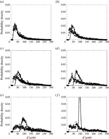
must be a statistical measure. In this section, a theoretical model for the Rayleigh–Taylor wavelength is rewritten simply as a time series. We subsequently test its suitability to predict the mean measured droplet sizes for all cases and therefore suggest a plausible fundamental mechanism of droplet formation in these flows. In addition, it is shown that for certain conditions the model is also able to recover the full distribution of experimentally measured droplet size.
5.1. The Rayleigh–Taylor mechanism in turbulent flows
Following the approach of Varga et al. (Reference Varga, Lasheras and Hopfinger2003), the acceleration of ligaments from the main liquid jet can be written using
 $$\begin{eqnarray}a=\frac{{\it\rho}_{g}\left(U_{g}(1+({\it\rho}_{g}/{\it\rho}_{l})^{1/2})-U_{l}\right)^{2}}{{\it\rho}_{l}b},\end{eqnarray}$$
where
 $U_{g}$
is the mean gas-phase velocity and
 $U_{l}$
the liquid jet velocity.
Experimental evidence from Varga et al. (Reference Varga, Lasheras and Hopfinger2003) suggested that on average, the thickness of liquid ligaments (b) was of the order of
 ${\it\lambda}_{1}/10$
and this order of magnitude was also confirmed through our experiments as outlined at the end of § 4.2. This leads to an expression for the acceleration of liquid ligaments off the main jet in terms of
 ${\it\lambda}_{1}$
as shown in
 $$\begin{eqnarray}a=\frac{10{\it\rho}_{g}\left(U_{g}(1+({\it\rho}_{g}/{\it\rho}_{l})^{1/2})-U_{l}\right)^{2}}{{\it\rho}_{l}{\it\lambda}_{1}},\end{eqnarray}$$
where
 ${\it\lambda}_{RT}$
can be written as
 $$\begin{eqnarray}{\it\lambda}_{RT}=2{\rm\pi}\left(\frac{3{\it\sigma}_{l}}{{\it\rho}_{l}a}\right)^{1/2}.\end{eqnarray}$$
In the absence of flow-field measurements,
 $U_{g}$
is the mean gas-phase velocity. However here, equations (5.2) and (5.3) can be rewritten as a time series, given that raw velocity data is available, such that
 $$\begin{eqnarray}\displaystyle & \displaystyle a(t)=\frac{10{\it\rho}_{g}\left(u_{g}(t)(1+({\it\rho}_{g}/{\it\rho}_{l})^{1/2})-U_{l}\right)^{2}}{{\it\rho}_{l}{\it\lambda}_{1}} & \displaystyle\end{eqnarray}$$
 $$\begin{eqnarray}\displaystyle & \displaystyle {\it\lambda}_{RT}(t)=2{\rm\pi}\left(\frac{3{\it\sigma}_{l}}{{\it\rho}_{l}a(t)}\right)^{1/2} & \displaystyle\end{eqnarray}$$
 $u_{g}(t)$
are representative.
Reconstructing a time series of
 ${\it\lambda}_{RT}$
therefore allows for a construction of a probability density function (PDF) of
 ${\it\lambda}_{RT}$
as well as for a determination of a number of mean calculations of
 ${\it\lambda}_{RT}$
. A key aim here is to determine a global constant that can be used to match the mean droplet sizes measured from the imaging system to model mean estimates as determined from the calculated time series of
 ${\it\lambda}_{RT}$
such that:
 $$\begin{eqnarray}\displaystyle & \displaystyle \mathit{SMD}=\frac{{\it\lambda}_{RT32}}{C_{SMD}} & \displaystyle\end{eqnarray}$$
 $$\begin{eqnarray}\displaystyle & \displaystyle d10=\frac{{\it\lambda}_{RT10}}{C_{D10}} & \displaystyle\end{eqnarray}$$
 ${\it\lambda}_{RT32}$
is a Sauter mean calculation of the
 ${\it\lambda}_{RT}$
time series and
 ${\it\lambda}_{RT10}$
is the arithmetic mean of
 ${\it\lambda}_{RT}$
. The values of SMD and
 $d10$
(arithmetic mean diameter) are the known, measured means such that the values of
 $C_{SMD}$
and
 $C_{D10}$
are values determined from the experimental data by normalizing the theoretical mean wavelength estimates by the measured mean diameters.
It was found by Varga et al. (Reference Varga, Lasheras and Hopfinger2003) that
 $C_{SMD}\sim 5$
regardless of flow conditions though
 ${\it\lambda}_{RT}$
was an instantaneous measurement as opposed to a mean of a model estimate as is done here. In addition, the reader is reminded that in the experiments of Varga et al. (Reference Varga, Lasheras and Hopfinger2003) the geometry of the air-assisted atomizer was fixed, in the sense that the liquid jet was always in the middle of the coflowing air, thereby likely resulting in a nearly constant turbulence intensity and thus constant ratio of (
 $\mathit{We}^{\prime }/\mathit{We}$
) amongst all cases.
5.2. Choice of
 ${\it\lambda}_{RT}$
normalization values

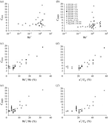
Figure 12(a) shows the
 $d10$
normalization value (
 $C_{D10}$
) used to match the mean Rayleigh–Taylor wavelength (
 ${\it\lambda}_{RT10}$
) to the measured
 $d10$
plotted versus the turbulent Weber number
 $\mathit{We}^{\prime }$
and figure 12(b) shows the analogous plot for
 $C_{SMD}$
. The calculations of
 $C_{SMD}$
determined by the current experiments are plotted alongside the estimates of Varga et al. (Reference Varga, Lasheras and Hopfinger2003) (codenamed ‘Var’ on figure 12
b) as well as measurements of Engelbert et al. (Reference Engelbert, Hardalupas and Whitelaw1995). Note that it has been assumed here that all cases of the literature have a turbulence intensity of roughly 17 % as suggested by Lasheras et al. (Reference Lasheras, Villermaux and Hopfinger1998). The reader should note that in Engelbert et al. (Reference Engelbert, Hardalupas and Whitelaw1995) values of
 ${\it\lambda}_{1}$
, which are required for the calculation of
 ${\it\lambda}_{RT}$
, were not provided but values of wave frequency
 $f_{W}$
were reported for a number of cases. Therefore, figure 12(b,e,f) use cases ‘s5’, ‘s6’, ‘s8’ and ‘s9’ (Engelbert et al.
Reference Engelbert, Hardalupas and Whitelaw1995). An assumption must also be made with regards to the velocity at which the waves on the liquid jet surface travel. Assumption 1 is that the wave travels at the ‘cluster velocity’ (
 $V_{C}$
) reported by Engelbert et al. (Reference Engelbert, Hardalupas and Whitelaw1995), hence yielding
 ${\it\lambda}_{1}=V_{C}/f_{W}$
. Assumption 2 is that close to the exit of the liquid jet, where the primary instability develops, the liquid is still travelling close to the ejected liquid jet velocity, hence providing
 ${\it\lambda}_{1}=U_{l}/f_{W}$
. Utilizing the SMD values reported at the spray centreline for each of the cases in Engelbert et al. (Reference Engelbert, Hardalupas and Whitelaw1995) and comparing with
 ${\it\lambda}_{RT}$
calculated from the two assumptions used for
 ${\it\lambda}_{1}$
, yields the results for ‘Eng.A1’ and ‘Eng.A2’ for assumptions 1 and 2, respectively, shown in figure 12(b,e,f).
Model normalization value
 $C_{D10}$
and
 $C_{SMD}$
plotted versus the turbulent Weber number (
 $\mathit{We}^{\prime }$
) (a,b),
 $C_{D10}$
plotted versus the ratio (
 $\mathit{We}^{\prime }/\mathit{We}$
) (c) and local turbulence intensity (
 $u^{\prime }/U_{g}$
) (d) and
 $C_{SMD}$
plotted versus
 $\mathit{We}^{\prime }/\mathit{We}$
(e) and the local turbulence intensity
 $u^{\prime }/U_{g}$
( f) for cases of table 1.

As seen both through figure 12(a,b), as the mean Weber number increases, it is clear that the influence of
 $\mathit{We}^{\prime }$
on the choice of the model normalization value begins to diminish and this is clear both through these experiments and those of Engelbert et al. (Reference Engelbert, Hardalupas and Whitelaw1995) and Varga et al. (Reference Varga, Lasheras and Hopfinger2003), where Varga et al. (Reference Varga, Lasheras and Hopfinger2003) state that the mean Weber number does not influence the ratio of droplet size to
 ${\it\lambda}_{RT}$
. Observation of figure 12(c–f) explains the apparent reason for this. For the extremely high-mean-Weber-number cases of Engelbert et al. (Reference Engelbert, Hardalupas and Whitelaw1995) and Varga et al. (Reference Varga, Lasheras and Hopfinger2003) the turbulent Weber number with respect to the mean
 $\mathit{We}^{\prime }/\mathit{We}=u^{2}/U_{g}^{2}$
is low (
 ${<}0.06$
), therefore suggesting that reductions in droplet size are driven entirely due to mean shear where turbulent mixing does not contribute further to the process, unlike in high
 $\mathit{We}^{\prime }/\mathit{We}$
cases from these experiments, which can have an impact on atomization behaviour as was discussed earlier in § 4.2.2.
By observation of figure 12(e,f), it can be seen that using assumption 2 of Engelbert et al. shows excellent agreement with the experimental data presented here yielding a
 $C_{SMD}$
of approximately 3.5. Utilizing assumption 1 results in a
 $C_{SMD}$
equal to an average of approximately 6.5. However, this is likely an overestimate as the ‘cluster velocity’ was measured by Engelbert et al. (Reference Engelbert, Hardalupas and Whitelaw1995) as the velocity of packets shedding off of the main core, which will be travelling faster than the primary instability due to ligament acceleration. The results of Varga et al. (Reference Varga, Lasheras and Hopfinger2003) show an average of approximately
 $C_{SMD}=5$
, which is a very reasonable agreement with the results presented here, where in those studies
 ${\it\lambda}_{RT}$
was measured directly.
Plotting
 $C_{SMD}$
or
 $C_{D10}$
versus the local turbulence intensity
 $u^{\prime }/U_{g}$
as opposed to
 $\mathit{We}^{\prime }/\mathit{We}$
yields the same conclusions, demonstrating here that
 $u^{\prime }/U_{g}$
can also be considered as a relevant scaling parameter for these sprays. At higher local turbulence intensities, the ratio of the break-up time of the liquid column is proportional to the turbulent timescale as described in § 4.1 and, clearly, the degree of turbulent mixing is dictating a wide range of atomization phenomena, from liquid jet fragmentation, to ligament formation and finally to droplet size formation as shown here.
Given that all cases used here lie on these model curves, leads to new expressions
 $$\begin{eqnarray}\displaystyle & C_{SMD}=\left\{\begin{array}{@{}ll@{}}\displaystyle 100m_{1}\left(\frac{u^{\prime }}{U_{g}}\right)-5,\quad & \text{if}~(u^{\prime }/U_{g})>0.25\\ 3.5,\quad & \text{if}~(u^{\prime }/U_{g})<0.25\end{array}\right. & \displaystyle\end{eqnarray}$$
 $$\begin{eqnarray}\displaystyle & C_{D10}=\left\{\begin{array}{@{}ll@{}}\displaystyle 100m_{2}\left(\frac{u^{\prime }}{U_{g}}\right)-2.3,\quad & \text{if}~(u^{\prime }/U_{g})>0.25\\ 5,\quad & \text{if}~(u^{\prime }/U_{g})<0.25\end{array}\right. & \displaystyle\end{eqnarray}$$
 $d10$
and SMD over the range of
 $\mathit{We}$
and
 $\mathit{We}^{\prime }$
examined. However, the reader should recall that due to reasons discussed in § 4.2,
 ${\it\lambda}_{1}$
is taken to be a constant for a given mean Weber number case and therefore the change in
 $C_{D10}$
and
 $C_{SMD}$
with
 $\mathit{We}^{\prime }/\mathit{We}$
and
 $u^{\prime }/U_{g}$
is only true under that assumption. Written alternatively in terms of the ratio of
 $\mathit{We}^{\prime }/\mathit{We}$
:
 $$\begin{eqnarray}\displaystyle & C_{SMD}=\left\{\begin{array}{@{}ll@{}}\displaystyle 60\left(\frac{\mathit{We}^{\prime }}{\mathit{We}}\right),\quad & \text{if}~(\mathit{We}^{\prime }/\mathit{We})>0.06\\ 3.5,\quad & \text{if}~(\mathit{We}^{\prime }/\mathit{We})<0.06\end{array}\right. & \displaystyle\end{eqnarray}$$
 $$\begin{eqnarray}\displaystyle & C_{D10}=\left\{\begin{array}{@{}ll@{}}\displaystyle 48\left(\frac{\mathit{We}^{\prime }}{\mathit{We}}\right)+2,\quad & \text{if}~(\mathit{We}^{\prime }/\mathit{We})>0.06\\ 5,\quad & \text{if}~(\mathit{We}^{\prime }/\mathit{We})<0.06\end{array}\right. & \displaystyle\end{eqnarray}$$
 $m_{1}=1/3$
and
 $m_{2}=0.3$
yielding
 $m_{1}\sim m_{2}$
and
 $\mathit{SMD}_{model}={\it\lambda}_{RT}/C_{SMD}$
and
 $d10_{model}={\it\lambda}_{RT}/C_{D10}$
.
5.3. Droplet size distribution calculation based on
$C_{D10}$

The previous section has demonstrated that mean values of
 $d10$
and SMD are recoverable using the model presented here, however here it is shown that for certain conditions droplet distributions may also be recovered. Utilizing the value of
 $C_{D10}$
determined, a PDF of
 ${\it\lambda}_{RT}$
is calculated by generating a histogram from (5.5) using the measured nominal raw
 $u_{g}$
signal from the LDA data at the liquid jet injection location and normalizing each calculated value of
 ${\it\lambda}_{RT}$
by
 $C_{D10}$
such that the
 $d10$
of the
 ${\it\lambda}_{RT}$
PDF and the measured
 $d10$
are matched. This is done for all cases measured, with only the main key findings presented here.
Figure 13 shows PDFs of
 ${\it\lambda}_{RT}$
normalized by the appropriate value of
 $C_{D10}$
as determined in § 5.2. Figure 13(a) shows the excellent match of
 ${\it\lambda}_{RT}/C_{D10}$
with the measured droplet size PDF at high turbulence intensities or at high values of
 $\mathit{We}^{\prime }/\mathit{We}$
. A good match is also present for a
 $\mathit{We}^{\prime }/\mathit{We}$
of 17 and 12 %, while the match at 6 % begins to deteriorate although it is still reasonable. A limitation of these PDF calculations is that
 ${\it\lambda}_{RT}$
cannot reconstruct the full range of measured droplet sizes at low turbulence intensity as seen through figure 13(e,f) although the agreement at droplet sizes greater than
 $100~{\rm\mu}\text{m}$
is reasonable. However, in applications where there is substantial intermittency in the velocity field, and where gas-phase turbulence drives the atomization process, an estimate of droplet size distribution would be possible using this simple model.
Theoretical PDFs of
 ${\it\lambda}_{RT}/C_{D10}$
(line) and measured PDFs of spherical droplet sizes (*) for case D2U2 (
 $D_{l}=210~{\rm\mu}\text{m}$
and
 $U_{g}=31~\text{m}~\text{s}^{-1}$
) at all available
 $\mathit{We}^{\prime }/\mathit{We}$
(%) values: (a) 28 %; (b) 17 %; (c) 12 %; (d) 6 %; (e) 4 %; ( f) 0.1 %.

The inability of the PDF to capture low turbulence intensity data is practically due to the inherent assumption made here that every calculated
 ${\it\lambda}_{RT}$
value will result in one particular droplet size. As the distribution of velocity scales narrows with the drop in turbulence intensity, then the ability for the narrow-band PDF of velocity to reconstruct a wide band polydisperse droplet size distribution fails. However, this finding demonstrates that for any case with a turbulence intensity of approximately 25 % and greater (
 $\mathit{We}^{\prime }/\mathit{We}>6\,\%$
), utilizing an appropriate model normalization value which depends on
 $\mathit{We}^{\prime }/\mathit{We}$
and
 $u^{\prime }/U_{g}$
, only velocity information and interfacial instability quantities are required to reconstruct the full droplet size distribution. This has been found true over all liquid jet sizes and velocities.
To summarize this section, it is clear that the
 ${\it\lambda}_{RT}$
model is able to reproduce mean sizes with a well-defined trend as demonstrated in § 5.2 although the full measured droplet size distributions downstream are only possible at high turbulence intensities and thus high
 $\mathit{We}^{\prime }/\mathit{We}$
. Nevertheless, this well-defined model using experimental data as an input provides evidence that
 ${\it\lambda}_{RT}$
as well as the turbulence intensity and
 $\mathit{We}^{\prime }/\mathit{We}$
are key quantities which can be used to estimate downstream droplet size, and can be used in statistical models in highly turbulent environments.
6. Measurements and predictions of droplet population
Turbulence has been shown to decrease the break-up length significantly and shorten the formation distance of ligaments, while also reduce the droplet size. The decrease in droplet size can be defined as a function of the initial Rayleigh–Taylor wavelength, by accounting for the raw flow-field velocity and by using a normalization value proportional to
 $\mathit{We}^{\prime }/\mathit{We}$
.
Given that both spray development and droplet sizes are related to the underlying turbulence, it is reasonable to assume that the turbulent flow-field also affects the number of droplets that are generated per unit of time, as the primary liquid column fragments. This is of use as a fundamental measure of atomization efficiency at the primary break-up location. Novel experimental data reported here confirms the overall size of ligaments and droplets, and therefore physical scalings should be possible for the prediction of total droplet number in a turbulent air-assisted spray. In this section, we present results of the total object number per image (all ligaments and all droplets), averaged over all images, at the primary break-up length, as a function of the turbulence level, and attempt to isolate the physical mechanisms responsible for changes in particle concentration. Analysis is restricted to the primary break-up location in order to concentrate on atomization phenomena only, by avoiding effects of downstream dispersion.
6.1. Measurements of population
The total number of objects per image (the images of which, for this calculation have been cropped to an area of approximately
 $2.8~\text{mm}\times 2.8~\text{mm}$
) are counted by the image processing routine. A mean number of objects per image is computed for all objects over all images using the same image processing system described in Kourmatzis et al. (Reference Kourmatzis, Pham and Masri2014). The reader is reminded that each image has a separation of
 $200~{\rm\mu}\text{s}$
and 1000 images are collected for each case. The mean number of objects
 $N_{obj,mean}$
plotted in figure 14 is therefore the mean number over the field of view detailed above, at the image frame representative of break-up length for each respective case. Figure 14(a) shows the number of objects plotted versus the turbulence intensity for various cases of the
 $D_{l}=210~{\rm\mu}\text{m}$
jet. Regardless of the mean flow conditions, a linear relationship is apparent between the total number of objects counted and the turbulence intensity in the flow. This shows that as with the droplet size and break-up length, the total population of objects generated upon break-up is also proportional to turbulent scales, and this is true for both figure 14(a,b).
Mean number of objects at the break-up length counted and computed over the full acquisition time plotted versus turbulence intensity for various cases of table 1: (a) for a liquid jet
 $D_{l}=210~{\rm\mu}\text{m}$
; (b) for a liquid jet
 $D_{l}=413~{\rm\mu}\text{m}$
.

However here, higher mean flow values and thus higher overall Weber numbers tend to generate significantly more droplets. This likely occurs because of greater mean shear forces along the liquid jet surface which can strip off smaller objects more regularly. Therefore, the production of droplets from the liquid core is a balance between overall shear force at the interface which drives the generation of instabilities, and entrainment from the surrounding air, given that
 $u^{\prime }$
, defined through the turbulence intensity on figure 14, clearly increases the number of droplets present. Therefore, a consistent finding is that as with the break-up length and droplet size, the number of objects generated is also dictated by a balance of mean shear and turbulent fluctuations.
6.2. Theoretical predictions of object population
In order to better understand the fundamental mechanism responsible for the transfer of liquid from the jet to droplets, shown in figure 14, we develop a number of simple physical scaling models subject to a number of assumptions. One key assumption that must be made is regarding the shape of objects resulting from the break-up of the liquid core. A second assumption must be made with regards to the boundary layer which develops along the main liquid jet surface, given that this will partly dictate the nature of the interfacial instabilities. A set of physical scalings are provided here which deal with the above two assumptions and are detailed in table 3.
Assumptions for object number physical scaling models.

Assumption T1 is that the characteristic dimensions of all objects are related solely to the Rayleigh–Taylor wavelength. This implicitly assumes that any object detected at the break-up zone is roughly spherical and has been shed from an accelerating ligament. Based on experimental observations at the break-up location, this is an inaccurate assumption, given that most objects are non-spherical at the break-up vicinity and should therefore not be defined by
 ${\it\lambda}_{RT}$
, however we entertain this possibility here for the purposes of comparison. Assumption L1, is also defined using
 ${\it\lambda}_{RT}$
as the characteristic size, but assumes a laminar boundary layer at the liquid jet surface. Assumption T2 is that the boundary layer along the liquid jet as it breaks up is turbulent, and also assumes that the majority of objects produced are non-spherical. Observation of the images at the break-up location generally confirms this to be the case, with the majority of objects being classified as ligaments. In addition, the experimental data of § 4.2 demonstrated that on average, the length of ligaments is directly proportional to the primary instability wavelength
 $n{\it\lambda}_{1}$
where
 $n$
approaches unity at the end of the atomization process. As was determined in § 4.2, ligaments which break from the main liquid column will have a dimension dictated by
 ${\it\lambda}_{1}$
, and therefore we also assume that the thickness of ligaments is also dictated by the primary instability. Such an assumption bears physical relevance given that the thickness of liquid ligaments
 $b$
, were found to be roughly proportional to
 ${\it\lambda}_{1}$
(Varga et al.
Reference Varga, Lasheras and Hopfinger2003). These characteristic lengths are used to define the characteristic ligament lengths under assumption T2, where L2 also assumes that ligaments dominate the spray but that the boundary layer on the primary jet is laminar.
Utilizing assumption T2 of table 3 and employing conservation of mass whilst assuming a monodisperse distribution for simplicity yields
 $$\begin{eqnarray}{\it\rho}_{l}U_{l}\frac{D_{l}^{2}}{4}\propto {\it\rho}_{l}{\dot{N}}_{obj}{\it\lambda}_{1}\frac{{\it\lambda}_{1}^{2}}{4}\end{eqnarray}$$
in terms of the total objects present per unit time,
 ${\dot{N}}_{obj}$
. In this analysis, we examine the effect of mean shear on the generation of liquid objects for a fixed turbulence intensity. At the end of the section we discuss requirements to extend the scaling to account for turbulence intensity. Therefore, this yields the following proportionality:
 $$\begin{eqnarray}{\dot{N}}_{obj}\propto \frac{U_{l}D_{l}^{2}}{{\it\lambda}_{1}^{3}}.\end{eqnarray}$$
Following the findings of Raynal (Reference Raynal1997) as stated earlier in the paper yields (4.1), and as stated in § 4.2, for a turbulent boundary layer:
 $$\begin{eqnarray}{\it\lambda}_{1}\propto \frac{1}{U_{g}^{1/5}}.\end{eqnarray}$$
Substituting (6.3) into (6.2) and taking
 $U_{l}$
and
 $D_{l}$
to be constants here results in
 $$\begin{eqnarray}{\dot{N}}_{obj}\propto U_{g}^{3/5}.\end{eqnarray}$$
In the case of assumption T1, objects are assumed to be droplets and hence defined by
 ${\it\lambda}_{RT}$
resulting in
 $$\begin{eqnarray}\displaystyle & \displaystyle {\it\rho}_{l}U_{l}\frac{D_{l}^{2}}{4}\propto {\it\rho}_{l}{\dot{N}}_{obj}\frac{{\it\lambda}_{RT}^{3}}{3} & \displaystyle\end{eqnarray}$$
 $$\begin{eqnarray}\displaystyle & \displaystyle {\dot{N}}_{obj}\propto \frac{U_{l}D_{l}^{2}}{{\it\lambda}_{RT}^{3}}. & \displaystyle\end{eqnarray}$$
 $a$
’ in terms of
 ${\it\lambda}_{RT}$
, yields the proportionality
 $$\begin{eqnarray}{\it\lambda}_{RT}\propto \frac{1}{U_{g}U_{g}^{1/10}}.\end{eqnarray}$$
Substituting (6.7) into (6.6), the proportionality of the number of objects detected should then follow a scaling of the form
 $$\begin{eqnarray}{\dot{N}}_{obj}\propto U_{g}^{3.3}\end{eqnarray}$$
for constant liquid jet flow conditions and diameter.
Further details on deriving the expression for
 ${\it\lambda}_{RT}$
are detailed elsewhere (Varga et al.
Reference Varga, Lasheras and Hopfinger2003). The reader should note that for a laminar boundary layer, the correct proportionalities for
 ${\it\lambda}_{RT}$
and
 ${\it\lambda}_{1}$
are respectively given by
 $$\begin{eqnarray}\displaystyle & \displaystyle {\it\lambda}_{RT}\propto \frac{1}{U_{g}U_{g}^{1/4}} & \displaystyle\end{eqnarray}$$
 $$\begin{eqnarray}\displaystyle & \displaystyle {\it\lambda}_{1}\propto \frac{1}{U_{g}^{1/2}}. & \displaystyle\end{eqnarray}$$
Therefore, the increase in object number from one velocity to another should trend with
 $U_{g}^{n}$
where
 $n$
is defined in the following expression for all assumptions of table 3:
 $$\begin{eqnarray}{\dot{N}}_{obj}\propto \left\{\begin{array}{@{}ll@{}}U_{g}^{3.3},\quad & \text{T1}\\ U_{g}^{0.6},\quad & \text{T2}\\ U_{g}^{3.75},\quad & \text{L1}\\ U_{g}^{1.5},\quad & \text{L2}.\end{array}\right.\end{eqnarray}$$
An increase in velocity from
 $U_{g,1}$
to
 $U_{g,2}$
would correspond to an increase from
 ${\dot{N}}_{obj,1}$
to
 ${\dot{N}}_{obj,2}$
given by
 $$\begin{eqnarray}\frac{{\dot{N}}_{obj,2}}{{\dot{N}}_{obj,1}}=\frac{U_{g,2}^{n}}{U_{g,1}^{n}}\end{eqnarray}$$
where
 $n$
is given in equation set (6.11).
6.3. Comparison of theory to measurements
To compare with the experimental data, the mean number of objects measured must be converted to an equivalent ‘per unit time’ estimate. In order to accomplish this, an estimate of the overall velocity of all objects must be made. Given that these measurements have been taken at the break-up length, the relevant velocity is either the bulk liquid velocity or the ‘cluster velocity’, the latter of which has been empirically defined by Engelbert et al. (Reference Engelbert, Hardalupas and Whitelaw1995) as
 $V_{C}=0.29U_{slip}^{0.82}$
for water jets. Estimating
 $V_{C}$
using this expression yields 3.1, 4.5, 5.7 and
 $7.9~\text{m}~\text{s}^{-1}$
for D2U1, D2U2, D2U3 and D2U4, respectively. By observing instances of liquid advection at the break-up length, these velocity estimates are very reasonable. Use of the mean gas flow is a gross overestimate given the very large Stokes numbers of these fragments. The mean number of objects from the images (
 $N_{obj,mean}$
) is converted into a time normalized estimate as
 ${\dot{N}}_{obj}=N_{obj,mean}/\text{d}t$
where
 $\text{d}t=\text{d}x/V_{C}$
and
 $\text{d}x$
is the field of view size. Given that for all cases investigated here, the field of view is a constant, and this is a proportional scaling analysis,
 $\text{d}x$
is fixed to unity.
In order to test the model scaling estimates, an initial datum is taken at the lowest velocity available such that the initial
 ${\dot{N}}_{obj,1}$
is taken to be the number of objects per unit time measured for
 $U_{g}=22~\text{m}~\text{s}^{-1}$
. From the scalings of expression (6.11) the predicted number of objects can then be determined at all other velocities, where an example calculation procedure is shown in the following expression for assumption T1 of equation set (6.11) where the scaling is written for a step increase from 22 to
 $31~\text{m}~\text{s}^{-1}$
:
 $$\begin{eqnarray}{\dot{N}}_{obj,31\,\text{m}\,\text{s}^{-1},m}={\dot{N}}_{obj,22\,\text{m}\,\text{s}^{-1},exp}\frac{31^{3.3}}{22^{3.3}}\end{eqnarray}$$
where
 ${\dot{N}}_{obj,U\,\text{m}\,\text{s}^{-1},m}$
indicates the number of objects per unit time at a mean velocity of
 $U$
for the model calculation and
 ${\dot{N}}_{obj,U\,\text{m}\,\text{s}^{-1},exp}$
the number of objects per unit time at a mean velocity of
 $U$
from the experiment.
This comparison is done for three different turbulence intensity levels and the results are plotted in figure 15. Clearly, all physical scalings yield generally consistent trends. For turbulence intensities of 20 and 40 % models T1 and L1 are the worst at higher velocities, and it can generally be seen that the rate of increase of object number with mean velocity is too high. It could be argued that this poor agreement is due to the inherent erroneous assumption with those two models that the volume of all objects can be attributed to spherical droplets with a characteristic size of
 ${\it\lambda}_{RT}$
. Nevertheless, at lower mean velocities, models L1 and T1 yield a better agreement and this requires further investigation. Over all turbulence intensities, the scaling that yields consistently the best agreement in terms of the rate of increase in object number with mean velocity is that of L2 which assumes that all sizes are dictated by the primary instability wavelength
 ${\it\lambda}_{1}$
, and utilizes a laminar boundary-layer assumption, which in the vicinity of the break-up location, is clearly a reasonable approximation. However, in terms of absolute quantities at low velocities, assumptions utilizing
 ${\it\lambda}_{RT}$
as a relevant scale are also suitable. What is of main importance here is that utilizing instability scales to generate an estimate of object number yield excellent trends, though further work is required to improve the absolute estimates.
Measured mean number of objects at the break-up length per unit time (
 ${\dot{N}}_{obj}$
), alongside mean objects per unit time predicted from assumptions T1–T2 and L1–L2 of table 3 plotted versus the mean velocity for a turbulence intensity of 10, 20 and 40 % for
 $D_{l}=210~{\rm\mu}\text{m}$
cases: (a)
 $u^{\prime }/U_{g}=10$
(%); (b)
 $u^{\prime }/U_{g}=20$
(%); (c)
 $u^{\prime }/U_{g}=40$
(%).

The growth in the number of objects is highly dependent on the mean flow conditions which scaling L2 is able to predict in a fairly reasonable manner. However, as shown in figure 14, there still is a turbulence intensity dependency, which the simple scalings of equation set (6.11) do not account for. By observation of figure 14, it is clear that the mean object number
 $N_{obj,mean}$
(and for a fixed mean velocity, the mean number of objects per unit time
 ${\dot{N}}_{obj}$
) scales linearly with the turbulence intensity as
 $$\begin{eqnarray}N_{obj,mean}\propto c\left(\frac{u^{\prime }}{U_{g}}\right)+e\end{eqnarray}$$
where
 $e$
, the vertical axis intercept of figure 14 takes on a value which depends on the mean velocity and liquid jet diameter, and is therefore a function of these quantities but also likely the physical properties, the latter of which have not been varied here. In the analysis of figure 15, an experimental data point was used as a datum and therefore once an initial value of ‘
 $e$
’ is known (
 $e_{i}$
), all subsequent values of
 $e_{i+1}$
can be assumed to scale with
 $U_{g,i}^{n}/U_{g,i-1}^{n}$
. The value of ‘
 $c$
’ in (6.14), as seen through figure 14, is roughly constant with
 $U_{g}$
, however it does depend on the liquid jet diameter
 $D_{l}$
. The subscript ‘
 $i$
’ denotes a particular condition of the spray in terms of a mean velocity, where in the example of figure 15,
 $U_{g,1}=22~\text{m}~\text{s}^{-1}$
and
 $U_{g,2}=31~\text{m}~\text{s}^{-1}$
. Based on the analysis summarized in figure 15,
 $n=1.5$
should be reasonable however whether this scaling holds for extremely high mean velocities, where surface tension becomes irrelevant is unknown. Further work is clearly required in order to fully test the applicability of such a generic scaling and its relevance over a wide range of physical properties, however these physical scalings demonstrate the applicability of instability scales in particle concentration estimation.
7. Summary and conclusions
The effects of shear-driven turbulence on the atomization behaviour of a liquid jet have been examined using LDA/PDA and microscopic high-speed backlit imaging in a comprehensive experiment which allows for the variation of turbulence intensity at a range of fixed mean gas velocities. The addition of local turbulence results in a range of instantaneous Weber numbers which cover a range of break-up regimes over many integral timescales of the flow. Therefore, the use of a single overall Weber number to describe the atomization process is insufficient. The contribution has expanded the available knowledge of air-assisted atomization by statistically accounting for the effects of gas-phase turbulence on primary break-up, which has resulted in a set of new physical scalings while also key findings summarized as follows.
-
(a) The primary break-up length is dictated by the turbulent Weber number
$\mathit{We}^{\prime }$
and by the level of turbulence intensity. The break-up distance also shows a relationship between the mass of liquid injected to that of the surrounding air, confirming the theory of Lasheras et al. (Reference Lasheras, Villermaux and Hopfinger1998). For a given liquid jet diameter, above a turbulence intensity of approximately 20–25 % (
$\mathit{We}^{\prime }/\mathit{We}\sim 6\,\%$
) the ratio of break-up time to turbulent timescale
${\it\tau}_{B}/{\it\tau}$
is constant, whereas at low turbulence intensities the mean conditions are important. This shows the relevance of gas-phase turbulence while also the fuel to air ratio by mass in determining the break-up length, two quantities which are seldom used in current models of primary atomization. -
(b) The final size of ligaments is dictated by the wavelength of the primary instability
${\it\lambda}_{1}$
. However, a higher degree of fluctuations tends to accelerate the ligament size ‘convergence distance’ or formation distance in such a way that this convergence distance is directly proportional to the break-up length. This suggests that models for the break-up length can also be employed to predict the downstream distance it takes for ligaments to reach their final size. For the first time, this finding experimentally and quantitatively demonstrates the influence of gas-phase turbulence on ligament formation and confirms the relevance of the primary instability in defining ligament structures. -
(c) The final droplet sizes are much smaller than the primary instability wavelength (of the order of
$0.1{\it\lambda}_{1}$
) and can be globally related to a balance of the turbulent Weber number
$\mathit{We}^{\prime }$
and mean Weber number
$\mathit{We}$
. As
$\mathit{We}^{\prime }$
exceeds a value of approximately 6 % of
$\mathit{We}$
, a much wider range of break-up regimes is possible causing the final droplet size to reduce further. This reduction in droplet size for a particular mean
$\mathit{We}$
is attributed to a combination of Rayleigh–Taylor instabilities which occur over a wide range of velocity scales while also turbulent fluctuations acting on the scale of the liquid fragments. -
(d) Estimates of the mean droplet diameters (
$d10$
and SMD) in terms of
${\it\lambda}_{RT}$
and two normalization values (
$C_{D10}$
and
$C_{SMD}$
) are provided to account for the dependence of droplet size on turbulence intensity and Rayleigh–Taylor wavelength. Above a turbulence intensity of approximately 25 %, corresponding to a
$\mathit{We}^{\prime }/\mathit{We}$
of greater than approximately 6 %, the constants (
$C_{D10}$
and
$C_{SMD}$
) become dependent on
$u^{\prime }/U_{g}$
and thus
$\mathit{We}^{\prime }/\mathit{We}$
. A simple model has been developed which allows for the calculation of
$d10$
and SMD based on model estimates of an arithmetic mean
${\it\lambda}_{RT}$
and a Sauter mean
${\it\lambda}_{RT}$
. -
(e) A model for the Rayleigh–Taylor wavelength previously suggested in Varga et al. (Reference Varga, Lasheras and Hopfinger2003) has been extended as a PDF, and can reconstruct the measured droplet diameter PDF in cases where
$\mathit{We}^{\prime }$
influences the atomization process. This analysis has provided an extended physical insight into the use of the Rayleigh–Taylor wavelength in making model estimates of droplet size in highly turbulent flows. -
(f) The spray population can be approximately estimated through conservation of mass and by assuming that ligament sizes are defined by key instability wavelengths. Expression (6.11) gives a number of suggested analytical scalings for estimating droplet population according to different assumptions. This is a unique and simple scaling that provides an alternative approach to estimating particle concentration in terms of initial instability wavelengths, which merits further advanced development.


Acknowledgement
The work is funded by the Australian Research Council.
List of symbols
-
$a$
-
Ligament acceleration
-
$b$
-
Thickness of ligament
-
$C_{D10}$
-
Normalization constant for arithmetic mean
-
$C_{SMD}$
-
Normalization constant for Sauter mean
-
$d$
-
Droplet diameter
-
$D$
-
Air nozzle jet diameter
-
$D_{B}$
-
Generic fragment size
-
$D_{l}$
-
Liquid jet diameter
-
$D_{max}$
-
Major axis length of liquid object
-
$D_{min}$
-
Minor axis length of liquid object
-
$f_{W}$
-
Liquid jet wave frequency
-
$L$
-
Ligament length
-
$N_{obj,mean}$
-
Mean number of objects detected in field of view
-
$r$
-
Radial location
-
$Rh_{f}$
-
Air jet half-radius
-
$U_{g}$
-
Mean air jet velocity
-
$u_{g}$
-
Instantaneous air jet velocity
-
$u^{\prime }$
-
Root mean square of gas flow fluctuations
-
$U_{l}$
-
Bulk mean liquid jet velocity
-
$V_{C}$
-
Liquid cluster velocity
-
$X$
-
Downstream location
-
$X_{B}$
-
Mean break-up length
-
$X_{L}$
-
Mean ligament convergence length


Greek symbols
-
${\it\delta}_{g}$
-
Gaseous vorticity layer thickness
-
${\it\Delta}$
-
Boundary layer development length
-
${\it\eta}$
-
Kolmogorov scale
-
${\it\Lambda}$
-
Integral length scale
-
${\it\lambda}_{1}$
-
Primary instability wavelength
-
${\it\lambda}_{RT}$
-
Rayleigh–Taylor instability wavelength
-
${\it\mu}_{l}$
-
Liquid dynamic viscosity
-
${\it\mu}_{g}$
-
Gas dynamic viscosity
-
${\it\nu}_{l}$
-
Liquid kinematic viscosity
-
${\it\nu}_{g}$
-
Gas kinematic viscosity
-
${\it\rho}_{l}$
-
Liquid density
-
${\it\rho}_{g}$
-
Gas density
-
${\it\sigma}_{l}$
-
Surface tension
-
${\it\tau}$
-
Integral time scale
-
${\it\tau}_{b}$
-
Instantaneous break-up time
-
${\it\tau}_{B}$
-
Mean break-up time


Dimensionless numbers
-
$m$
-
Liquid to air mass ratio
-
$\mathit{Re}_{l}$
-
Liquid jet Reynolds number
-
$\mathit{Re}_{g}$
-
Gas jet Reynolds number
-
$\mathit{We}$
-
Mean exit Weber number
-
$\mathit{we}$
-
Instantaneous Weber number
-
$\mathit{We}^{\prime }$
-
Turbulent Weber number
-
$\mathit{We}_{t}$
-
‘Traditional’ turbulent Weber number