


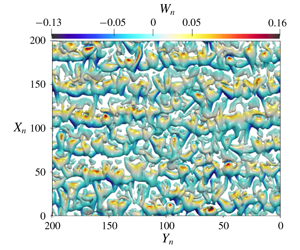


1 Introduction
Stably stratified flows are commonly observed in the atmospheric boundary layer (ABL) and typically occur during night-time due to radiative heat loss from the surface to clear skies or under cold climate conditions such as in the Arctic and Antarctic. Stratified flows play a vital role in reliable weather prediction pertaining to air quality, agriculture and aviation (Fernando & Weil Reference Fernando and Weil2010). A plethora of numerical and experimental studies have been conducted for stably stratified atmospheric boundary layer flows over flat terrain (e.g. Coleman, Ferziger & Spalart Reference Coleman, Ferziger and Spalart1990; Mason & Derbyshire Reference Mason and Derbyshire1990; Kosović & Curry Reference Kosović and Curry2000; Beare et al. Reference Beare, Macvean, Holtslag, Cuxart, Esau, Golaz, Jimenez, Khairoutdinov, Kosovic and Lewellen2006; Shah & Bou-Zeid Reference Shah and Bou-Zeid2014). However, stably stratified flows over non-flat terrain are relatively less explored.
One of the simplest configurations of that kind are slope flows, also known as drainage winds, that are caused by a horizontal air temperature gradient due to a misalignment of the stratification and main shear direction over non-flat terrain. During night-time, the ABL becomes stably stratified after several hours of prior near-surface radiative cooling, which triggers a downslope flow over sloped terrain, also called a katabatic wind (see e.g. Whiteman Reference Whiteman1990). After sunrise, while the stable background stratification still persists, the surface starts to become heated, giving rise to stably stratified upslope flows, also known as anabatic flows. This configuration, however, does not last very long, since the stable atmospheric boundary layer (SABL) transitions to a well-mixed convective boundary layer due to ongoing surface heating (cf. Banta Reference Banta1984). Anabatic flows under these thermally unstable daytime atmospheric conditions have been discussed in Whiteman (Reference Whiteman1990, Reference Whiteman2000), Monti et al. (Reference Monti, Fernando, Princevac, Chan, Kowalewski and Pardyjak2002) and Fernando et al. (Reference Fernando, Pardyjak, Di Sabatino, Chow, De Wekker, Hoch, Hacker, Pace, Pratt and Pu2015), but they are not the subject of the current study, in which the term ‘anabatic flows’ presupposes the presence of a stably stratified atmosphere. A more in-depth treatment of the observational and phenomenological approach to diurnal mountain wind systems in which anabatic flows occur can also be found in the works by Zardi & Whiteman (Reference Zardi and Whiteman2013) and Serafin et al. (Reference Serafin, Adler, Cuxart, De Wekker, Gohm, Grisogono, Kalthoff, Kirshbaum, Rotach and Schmidli2018).
The canonical flow model to capture the main dynamics of such anabatic as well as katabatic flows is the one proposed by Prandtl (Reference Prandtl1942, Reference Prandtl1952), which treats the problem as a viscous stably stratified fluid layer flowing over an inclined doubly infinite planar surface cooled or heated from the bottom with a constant temperature. The exact buoyancy and velocity solutions arising from the Prandtl model are both sinusoidal profiles damped exponentially with growing height (Fedorovich & Shapiro Reference Fedorovich and Shapiro2009). The solution gives rise to a strong near-surface jet along the slope direction, which is capped by a weak reverse flow as depicted in figure 1 for both the anabatic and katabatic conditions. Despite its simplicity, the Prandtl model has been found to capture qualitatively the structure of katabatic slope winds normal to the slope observed in nature (Defant Reference Defant1949a,Reference Defantb). However, further adjustments through introduction of constant eddy viscosity and diffusivity into the Prandtl model did not result in improved predictions with respect to field observations (Grisogono & Oerlemans Reference Grisogono and Oerlemans2001a,Reference Grisogono and Oerlemansb).
Base-flow profiles for slope flows under Prandtl’s model. (a) Sketch of slope-flow geometry and the rotated coordinate system:  $z^{\prime }$ represents the vertical axis of the coordinate system before rotation, i.e. parallel to the gravity vector. The katabatic and anabatic configurations differ only in the sign of their surface buoyancy flux and the resulting flow profiles. The figure is not drawn to scale. (b) Normalised velocity and buoyancy profiles as well as their slope-normal gradients.

Stable stratification of the background environment is essential for the formation of anabatic and katabatic winds over non-flat terrain. However, despite the significance of the stably stratified conditions, its representation in numerical weather models has been a technical challenge for a long while. Ad hoc remedies to improve the representation of SABLs are known to erode the representation of other processes (Mahrt Reference Mahrt1998; Sandu et al. Reference Sandu, Beljaars, Bechtold, Mauritsen and Balsamo2013; Steeneveld Reference Steeneveld2014). The SABL is typically divided into weakly stable (WSABL) or very stable (VSABL) regimes. This qualitative classification was introduced by Mahrt (Reference Mahrt1998) to highlight the technical challenges in modelling the very stable regime, also referred to as ‘strongly stratified’. It is generally accepted that we have a reasonable representation of WSABL over flat homogeneous terrain through the Monin–Obukhov similarity theory (MOST) (Monin & Obukhov Reference Monin and Obukhov1954) and the local scaling hypothesis of Nieuwstadt (Reference Nieuwstadt1984). However, a comprehensive understanding of VSABLs over non-flat terrain still remains elusive, which has been attributed to the intermittency of turbulence and mixing processes under very stable conditions (Fernando & Weil Reference Fernando and Weil2010; Mahrt Reference Mahrt2014).
Numerous numerical studies on katabatic and anabatic flows under Prandtl’s model have been published in the literature. The first large-eddy simulation for anabatic flows was conducted by Schumann (Reference Schumann1990), who was able to observe en masse oscillations of instantaneous flow quantities in the numerical results with characteristic frequency of  $N\sin \unicode[STIX]{x1D6FC}$, in agreement with data from field experiments (Turner Reference Turner1979). These oscillations were shown to persist in numerical simulations of turbulent Prandtl-type slope flow starting from rest (Fedorovich & Shapiro Reference Fedorovich and Shapiro2017).
Fedorovich & Shapiro (Reference Fedorovich and Shapiro2009) were the first to conduct direct numerical simulations (DNS) of a turbulent analogue of the Prandtl model for anabatic and katabatic conditions. They proposed a dimensionless parameter called the ‘integral slope-flow Reynolds number’ that is derived from an integral dynamic similarity constraint applicable to flows over a constant slope driven by a uniform surface buoyancy flux. The integral Reynolds number lumps together the effect of slope angle, surface buoyancy flux, viscosity and background stratification in a single dimensionless number. Fedorovich & Shapiro also introduced a dimensionless flow forcing parameter that is a measure of the ratio between energy production at the surface and the work against buoyancy and viscous forces. For a given slope angle, flow is expected to be more turbulent at higher values of the flow forcing parameter. Several DNS of slope flows were performed for integral Reynolds number in the range of 3000–10 000. Mean profiles of turbulent katabatic flows were found to be structurally more similar to the laminar Prandtl model than the mean profiles of anabatic flows were. Unlike flat terrain, where a constancy of the turbulent fluxes led to the development of similarity theory, Fedorovich & Shapiro (Reference Fedorovich and Shapiro2009) found no evidence of constancy of fluxes in slope flows, which casts doubt on the applicability of MOST-based surface parametrisations for non-flat terrain. However, the issue of to what extent MOST is inapplicable to slope flows remains unresolved. Giometto et al. (Reference Giometto, Katul, Fang and Parlange2017) complemented the work of Fedorovich & Shapiro by conducting DNS of slope flows for prescribed surface buoyancy as opposed to the prescribed buoyancy flux used in Fedorovich & Shapiro (Reference Fedorovich and Shapiro2009). Giometto et al. performed a detailed budget analysis for turbulent kinetic energy and fluxes, and they too did not observe a constant flux layer. Giometto et al. (Reference Giometto, Katul, Fang and Parlange2017) also showed that, at slope angles lower than  $30^{\circ }$, the anabatic and katabatic flows differ in turbulence statistics and in the way the flow returns to isotropy.
Several numerical and experimental results on instabilities in different stably stratified flow configurations have appeared in the recent literature. Deloncle, Chomaz & Billant (Reference Deloncle, Chomaz and Billant2007) carried out a numerical analysis of the inviscid stability for a stably stratified flow over a horizontal surface, whereas Facchini et al. (Reference Facchini, Favier, Le Gal, Wang and Le Bars2018) studied the stability of Couette flows with stable stratification via linear analysis, experiments and DNS. Chen, Bai & Le Dizès (Reference Chen, Bai and Le Dizès2016) investigated stably stratified horizontal boundary layer flows on a vertical wall; in all those cases, the direction of stratification was either parallel or orthogonal to the shear and base-flow directions. Candelier, Le Dizès & Millet (Reference Candelier, Le Dizès and Millet2011, Reference Candelier, Le Dizès and Millet2012) analysed the inviscid stability for a case where the direction of stratification was orthogonal to the base-flow direction but makes an oblique angle with the plane of shear, identifying both Kelvin–Helmholtz (KH) and radiative instabilities generated by a Bickley jet ejected onto a sloping surface. The Prandtl model for slope flows is distinct from all these aforementioned flow configurations because the direction of stratification is oblique to both the base-flow direction and the direction of shear due to the inclination of the surface. In addition, heat conduction is a principal component of the Prandtl model, which is not considered in the aforementioned studies.
In a recent study, we have investigated the linear stability of the Prandtl model for katabatic slope flows and introduced a new dimensionless parameter,  $\unicode[STIX]{x1D6F1}_{s}$, the so-called stratification perturbation parameter, which is used alongside the slope angle and Prandtl number to characterise the stability behaviour of such flows (Xiao & Senocak Reference Xiao and Senocak2019). The parameter
 $\unicode[STIX]{x1D6F1}_{s}$ is related to the flow forcing parameter
 $Fp_{B}$ introduced in Fedorovich & Shapiro (Reference Fedorovich and Shapiro2009) through the Prandtl number
 $Pr$ as
 $\unicode[STIX]{x1D6F1}_{s}=Fp_{B}\,Pr$. We have attributed the complexity of the katabatic slope flow’s linear response to infinitesimal perturbations to the disturbance to the background stratification due to the thermal forcing at the surface. The complexity of the resulting flow is somewhat unexpected because the combined effect of surface cooling and stable background stratification are a priori presumed to be both stabilising contributions. On the other hand, the potential existence of instabilities in anabatic flows would be a more expected outcome due to the presence of heating instead of cooling at the surface. Indeed, numerous numerical and experimental studies for the stability of natural convection flows in the absence of stable stratification on a heated inclined surface have appeared in the literature.
Sparrow & Husar (Reference Sparrow and Husar1969) reported the observation of longitudinal vortices on a heated plate when inclined at a low angle, and Lloyd & Sparrow (Reference Lloyd and Sparrow1970) observed the transition of these vortices into travelling waves at larger inclination angles, which is analogous to the stability behaviour of katabatic flows established by Xiao & Senocak (Reference Xiao and Senocak2019). Subsequently, linear stability analysis (LSA) and further experiments for boundary layer flows over a heated inclined surface have been carried out by Haaland & Sparrow (Reference Haaland and Sparrow1973), Pera & Gebhart (Reference Pera and Gebhart1973) and Iyer & Kelly (Reference Iyer and Kelly1974), establishing neutral stability boundaries for both instability types depending on inclination angle, with good agreement between the experimental data and numerical results. Clever & Busse (Reference Clever and Busse1977) went beyond the primary stability analysis for the base flow on a heated inclined layer and also studied the stability of the convection rolls that are the primary instabilities of the base flow. The effect of flow instability on surface momentum and heat transfer rates has been studied by Chen & Tzuoo (Reference Chen and Tzuoo1982), whereas Lin (Reference Lin2001) investigated the evolution of the vortex instability with variation to different dimensionless flow parameters. Beyond the study of linear flow stability, Lloyd & Sparrow (Reference Lloyd and Sparrow1970) have also carried out experiments for the transition and turbulent regimes of natural convection over inclined plates, obtaining measurement data for mass transfer rates at the surface. However, the previous studies focused on natural convection with an eye toward engineering applications and did not consider the effect of stable background stratification, a common feature of geophysical flows.
In the present work, we continue our investigation of the stability of the Prandtl model for stratified slope flows with the anabatic case and complement our earlier study (Xiao & Senocak Reference Xiao and Senocak2019) that was focused on the katabatic case. The current investigation is imperative to better comprehend the stability characteristics of the Prandtl model because, as observed by Fedorovich & Shapiro (Reference Fedorovich and Shapiro2009), despite only differing in the sign of their surface buoyancy flux and thus laminar flow profiles, the mean profiles of katabatic and anabatic flows differ significantly from each other in the turbulent regime, with the katabatic version showing a closer resemblance to the Prandtl solution. Similar to the approach that we pursued in Xiao & Senocak (Reference Xiao and Senocak2019), we first apply LSA to identify the instability boundaries, and subsequently carry out DNS to support the findings of the LSA and visualise the nature of flow instabilities. We further conduct asymptotic analyses to identify the primary instability mechanisms in slope flows.
2 Governing equations
The idealised slope-flow configuration is shown in figure 1(a), where  $\unicode[STIX]{x1D6FC}$ is the slope angle, gravity acts in the vertical direction and
 $B_{S}$ is the constant buoyancy flux imposed on the surface. For ease of analysis, the problem is studied in a rotated Cartesian coordinate system whose
 $x$ axis is aligned with the planar inclined surface. We let
 $u$ be the along-slope (longitudinal),
 $v$ the cross-slope (transverse) and
 $w$ the slope-normal velocity components, such that
 $u_{i}=[u,v,w]$ is the velocity vector. The gravity vector in the rotated coordinate system is then given by
 $g_{i}=(g_{1},g_{2},g_{3})=[\sin \unicode[STIX]{x1D6FC},0,\cos \unicode[STIX]{x1D6FC}]$. The potential temperature, buoyancy and its frequency are denoted by
 $\unicode[STIX]{x1D703}$,
 $b$ and
 $N$, respectively;
 $N$ is also known as the Brunt–Väisälä frequency, defined as
 $N=\sqrt{(g/\unicode[STIX]{x1D6E9}_{r})\,\unicode[STIX]{x2202}\unicode[STIX]{x1D6E9}_{e}/\unicode[STIX]{x2202}z^{\prime }}$, and
 $N^{2}$ is used as a measure of the stratification. The buoyancy is related to the potential temperature as
 $b=g(\unicode[STIX]{x1D6E9}-\unicode[STIX]{x1D6E9}_{e})/\unicode[STIX]{x1D6E9}_{r}$, where
 $\unicode[STIX]{x1D6E9}_{r}$ is a reference potential temperature and
 $\unicode[STIX]{x1D6E9}_{e}$ is the environmental potential temperature. The kinematic viscosity and thermal diffusivity of the fluid are denoted by
 $\unicode[STIX]{x1D708}$ and
 $\unicode[STIX]{x1D6FD}$, respectively, and are assumed to be constant. Following the presentation in Fedorovich & Shapiro (Reference Fedorovich and Shapiro2009), the momentum and the buoyancy balance equations with a Boussinesq approximation are written as follows:
 $$\begin{eqnarray}\displaystyle & \displaystyle \frac{\unicode[STIX]{x2202}u_{i}}{\unicode[STIX]{x2202}t}+\frac{\unicode[STIX]{x2202}u_{i}u_{j}}{\unicode[STIX]{x2202}x_{j}}=-\frac{1}{\unicode[STIX]{x1D70C}}\frac{\unicode[STIX]{x2202}p}{\unicode[STIX]{x2202}x_{i}}+g_{i}b+\frac{\unicode[STIX]{x2202}}{\unicode[STIX]{x2202}x_{j}}\left(\unicode[STIX]{x1D708}\frac{\unicode[STIX]{x2202}u_{i}}{\unicode[STIX]{x2202}x_{j}}\right), & \displaystyle\end{eqnarray}$$
 $$\begin{eqnarray}\displaystyle & \displaystyle \frac{\unicode[STIX]{x2202}b}{\unicode[STIX]{x2202}t}+\frac{\unicode[STIX]{x2202}u_{j}b}{\unicode[STIX]{x2202}x_{j}}=\frac{\unicode[STIX]{x2202}}{\unicode[STIX]{x2202}x_{j}}\left(\unicode[STIX]{x1D6FD}\frac{\unicode[STIX]{x2202}b}{\unicode[STIX]{x2202}x_{j}}\right)-N^{2}g_{j}u_{j}. & \displaystyle\end{eqnarray}$$
The conservation-of-mass principle is imposed by a divergence-free velocity field,
 $$\begin{eqnarray}\frac{\unicode[STIX]{x2202}u_{i}}{\unicode[STIX]{x2202}x_{i}}=0.\end{eqnarray}$$
In the following, the position and velocity vector components  $(x_{i})^{\text{T}}$ and
 $(u_{i})^{\text{T}}$ are denoted as
 $(x,y,z)^{\text{T}}$ and
 $(u,v,w)^{\text{T}}$, respectively. At the surface, a positive buoyancy flux
 $B_{s}$ is imposed to create anabatic flow conditions. In the Prandtl model, equation (2.1) reduces to a balance between buoyancy and diffusion of along-slope momentum; and (2.2) reduces to a balance between along-slope momentum and diffusion of buoyancy. For the case with a constant buoyancy flux at the surface, Shapiro & Fedorovich (Reference Shapiro and Fedorovich2004) provide the following solution of the laminar flow:
 $$\begin{eqnarray}\displaystyle & \displaystyle u_{n}=u/u_{0}=\sqrt{2}\sin (z_{n}/\sqrt{2})\exp (-z_{n}/\sqrt{2}), & \displaystyle\end{eqnarray}$$
 $$\begin{eqnarray}\displaystyle & \displaystyle b_{n}=b/b_{0}=\sqrt{2}\cos (z_{n}/\sqrt{2})\exp (-z_{n}/\sqrt{2}), & \displaystyle\end{eqnarray}$$
where  $z_{n}=z/l_{0}$,
 $u_{n}$ and
 $b_{n}$ are non-dimensional height, velocity and buoyancy, respectively. According to (2.4) and (2.5), Prandtl’s flow profile is an exponentially damped sinusoid with infinitely many inflection points. It satisfies both Rayleigh’s and Fjørtoft’s necessary criterion for instability, which opens the possibility for inviscid inflection instabilities (Schmid & Henningson Reference Schmid and Henningson2001; Drazin & Reid Reference Drazin and Reid2004). The profiles of
 $u_{n}$ and
 $b_{n}$ and their slope-normal derivatives are shown in figure 1(b).
The corresponding scales governing the laminar flow are given as (Fedorovich & Shapiro Reference Fedorovich and Shapiro2009)
 $$\begin{eqnarray}\displaystyle & \displaystyle l_{0}=Pr^{-1/4}\unicode[STIX]{x1D708}^{1/2}N^{-1/2}\sin ^{-1/2}\unicode[STIX]{x1D6FC}, & \displaystyle\end{eqnarray}$$
 $$\begin{eqnarray}\displaystyle & \displaystyle u_{0}=Pr^{1/4}\unicode[STIX]{x1D708}^{-1/2}N^{-3/2}B_{s}\sin ^{-1/2}\unicode[STIX]{x1D6FC}, & \displaystyle\end{eqnarray}$$
 $$\begin{eqnarray}\displaystyle & \displaystyle b_{0}=Pr^{3/4}\unicode[STIX]{x1D708}^{-1/2}N^{-1/2}B_{s}\sin ^{-1/2}\unicode[STIX]{x1D6FC}, & \displaystyle\end{eqnarray}$$
where  $Pr=\unicode[STIX]{x1D708}/\unicode[STIX]{x1D6FD}$. A time scale
 $t_{0}=l_{0}/|u_{0}|=\sqrt{\unicode[STIX]{x1D708}\unicode[STIX]{x1D6FD}}N|B_{s}|^{-1}$ can also be defined from the above scales. We can see from (2.6)–(2.8) that the length scale is independent of the surface flux
 $B_{s}$, whereas the magnitudes of both the reference velocity and buoyancy scale vary linearly with
 $B_{s}$. As expected, the characteristic length scale increases with diminishing background stratification
 $N$, leading to an infinitely thick boundary layer of infinite strength in the neutral limit. It is interesting to note, however, that the time and frequency scales for the laminar Prandtl flow, as given by
 $l_{0}/u_{0}$ or
 $u_{0}/l_{0}$, are independent of the slope angle
 $\unicode[STIX]{x1D6FC}$.
3 Linear stability analysis
Linearising (2.2) around Prandtl’s laminar solution given by (2.4) and (2.5), and assuming that disturbances to the base flow given by Prandtl’s solution are waves of the form  $\boldsymbol{q}(x,y,z,t)=\hat{\boldsymbol{q}}(\boldsymbol{z})\text{e}^{\unicode[STIX]{x1D714}t+\text{i}(k_{x}x+k_{y}y)}$, the resulting equations have the form
 $$\begin{eqnarray}\displaystyle & \displaystyle \text{i}k_{x}\hat{u} +\text{i}k_{y}\hat{v}+\frac{\unicode[STIX]{x2202}{\hat{w}}}{\unicode[STIX]{x2202}z}=0, & \displaystyle\end{eqnarray}$$
 $$\begin{eqnarray}\displaystyle & \displaystyle \unicode[STIX]{x1D714}\hat{u} +\text{i}u_{n}k_{x}\hat{u} +u_{n}^{\prime }{\hat{w}}=-\text{i}k_{x}\hat{p}+\frac{\unicode[STIX]{x1D70E}Pr}{\unicode[STIX]{x1D6F1}_{s}}\sin \unicode[STIX]{x1D6FC}\left(-(k_{x}^{2}+k_{y}^{2})\hat{u} +\frac{\unicode[STIX]{x2202}^{2}\hat{u} }{\unicode[STIX]{x2202}z^{2}}+\hat{b}\right), & \displaystyle\end{eqnarray}$$
 $$\begin{eqnarray}\displaystyle & \displaystyle \unicode[STIX]{x1D714}\hat{v}+\text{i}u_{n}k_{x}\hat{v}=-\text{i}k_{y}\hat{p}+\frac{\unicode[STIX]{x1D70E}Pr}{\unicode[STIX]{x1D6F1}_{s}}\sin \unicode[STIX]{x1D6FC}\left(-(k_{x}^{2}+k_{y}^{2})\hat{v}+\frac{\unicode[STIX]{x2202}^{2}\hat{v}}{\unicode[STIX]{x2202}z^{2}}\right), & \displaystyle\end{eqnarray}$$
 $$\begin{eqnarray}\displaystyle & \displaystyle \unicode[STIX]{x1D714}{\hat{w}}+\text{i}u_{n}k_{x}{\hat{w}}=-\frac{\unicode[STIX]{x2202}\hat{p}}{\unicode[STIX]{x2202}z}+\frac{\unicode[STIX]{x1D70E}Pr}{\unicode[STIX]{x1D6F1}_{s}}\sin \unicode[STIX]{x1D6FC}\left(-(k_{x}^{2}+k_{y}^{2}){\hat{w}}+\frac{\unicode[STIX]{x2202}^{2}{\hat{w}}}{\unicode[STIX]{x2202}z^{2}}+\hat{b}\cot \unicode[STIX]{x1D6FC}\right), & \displaystyle\end{eqnarray}$$
 $$\begin{eqnarray}\displaystyle & \displaystyle \unicode[STIX]{x1D714}\hat{b}+\text{i}u_{n}k_{x}\hat{b}+b_{n}^{\prime }{\hat{w}}=\frac{\unicode[STIX]{x1D70E}\sin \unicode[STIX]{x1D6FC}}{\unicode[STIX]{x1D6F1}_{s}}\left(-(k_{x}^{2}+k_{y}^{2})\hat{b}+\frac{\unicode[STIX]{x2202}^{2}\hat{b}}{\unicode[STIX]{x2202}z^{2}}-(\hat{u} +{\hat{w}}\cot \unicode[STIX]{x1D6FC})\right), & \displaystyle\end{eqnarray}$$
where  $\hat{u} ,~\hat{v},~{\hat{w}},~\hat{p}$ and
 $\hat{b}$ are flow disturbances varying along the slope-normal direction normalised by the flow scales given in (2.6)–(2.8), and
 $\unicode[STIX]{x1D70E}:=\text{sgn}(B_{s})$ is the sign of the surface buoyancy flux, which equals 1 for anabatic flows. The Prandtl base-flow solution and its derivative normal to the surface are denoted by
 $u_{n},u_{n}^{\prime }$ and
 $b_{n}^{\prime }$.
From (3.1)–(3.5), it is clear that there are three non-dimensional parameters characterising the idealised anabatic slope flow, which can also be confirmed independently by applying the Buckingham  $\unicode[STIX]{x03C0}$ theorem. These non-dimensional parameters are the Prandtl number
 $Pr$, the slope angle
 $\unicode[STIX]{x1D6FC}$ and the stratification perturbation parameter
 $\unicode[STIX]{x1D6F1}_{s}$ that was introduced in Xiao & Senocak (Reference Xiao and Senocak2019):
 $\unicode[STIX]{x1D6F1}_{s}$ is the ratio between the imposed surface buoyancy gradient
 $B_{s}/\unicode[STIX]{x1D6FD}$ and the background stratification
 $N^{2}$. This unique parameter is determined from the given flow parameters as follows:
 $$\begin{eqnarray}\unicode[STIX]{x1D6F1}_{s}\equiv \frac{|B_{s}|}{\unicode[STIX]{x1D6FD}N^{2}}.\end{eqnarray}$$
As mentioned earlier,  $\unicode[STIX]{x1D6F1}_{s}$ can also be related to the internal Froude number as
 $\unicode[STIX]{x1D6F1}_{s}=Fr\sqrt{Pr}$, and to the Richardson number as
 $\unicode[STIX]{x1D6F1}_{s}=\sqrt{Pr/Ri}$ using the flow scales defined in (2.6)–(2.8). However, it would be injudicious to use
 $Fr$ and
 $Ri$ for the Prandtl model because there are no externally imposed velocity or length scales in the flow problem. Parameter
 $\unicode[STIX]{x1D6F1}_{s}$ is related to the flow forcing parameter
 $Fp_{B}\equiv B_{s}\unicode[STIX]{x1D708}^{-1}N^{-2}$ introduced in Fedorovich & Shapiro (Reference Fedorovich and Shapiro2009) through the following relation:
 $\unicode[STIX]{x1D6F1}_{s}=Fp_{B}\,Pr$. Although these two parameters appear similar, they differ in the physical processes they represent:
 $Fp_{B}$ is a measure of energy input at the surface relative to the work done against buoyancy and viscous forces, whereas
 $\unicode[STIX]{x1D6F1}_{s}$ is a measure of the thermal perturbation to the background stratification at the surface.
The linearised equations can be written as a generalised eigenvalue problem as follows:
 $$\begin{eqnarray}\unicode[STIX]{x1D63C}(k_{x},k_{y})\hat{\boldsymbol{q}}(z)=\unicode[STIX]{x1D714}\unicode[STIX]{x1D63D}\hat{\boldsymbol{q}}(z).\end{eqnarray}$$
The complex disturbance amplitude vector  $\hat{\boldsymbol{q}}(z)=[\hat{u} (z),\hat{v}(z),{\hat{w}}(z),\hat{p}(z),\hat{b}(z)]^{\text{T}}$ only varies in the slope-normal direction, where
 $(\hat{u} ,\hat{v},{\hat{w}})$ are the along-slope, cross-slope (transverse) and slope-normal disturbance velocity components. The appropriate boundary conditions for this problem are no slip for disturbance velocities at
 $z=0$ and
 $z\rightarrow \infty$; and for buoyancy disturbance,
 $\unicode[STIX]{x2202}\hat{b}/\unicode[STIX]{x2202}z|_{0}=0$ and
 $\hat{b}|_{z\rightarrow \infty }=0$ are imposed. The slope-normal derivative of pressure disturbance
 $\hat{p}$ is also set to zero at both
 $z=0$ and
 $z\rightarrow \infty$. The generalised eigenvalue problem (3.7) is solved via a collocated spectral method using Chebyshev polynomials and an algebraic map to cover the semi-infinite domain
 $[0,\infty )$ (e.g. Schmid & Henningson Reference Schmid and Henningson2001). Two-hundred collocation points are used for discretisation, and the resulting generalised eigenvalue problem is solved with the help of MATLAB functions. Linear stability of the problem is associated with the real part of the eigenvalues
 $\unicode[STIX]{x1D714}$, where
 $\text{Re}\{\unicode[STIX]{x1D714}\}>0$ represents a positive exponential growth for the corresponding eigenmode, thus an unstable mode. The imaginary part of
 $\unicode[STIX]{x1D714}$ is the temporal oscillation frequency for the corresponding eigenmode, and
 $\text{Im}\{\unicode[STIX]{x1D714}\}=0$ represents a stationary mode.
Growth-rate contours depending on wavenumber vectors  $k_{x}$ and
 $k_{y}$ at different slope angles for
 $Pr=0.71$: (a)
 $\unicode[STIX]{x1D6FC}=2^{\circ }$,
 $\unicode[STIX]{x1D6F1}_{s}=1.7$; (b)
 $\unicode[STIX]{x1D6FC}=5^{\circ }$,
 $\unicode[STIX]{x1D6F1}_{s}=2.15$; (c)
 $\unicode[STIX]{x1D6FC}=9.5^{\circ }$,
 $\unicode[STIX]{x1D6F1}_{s}=3.2$; and (d)
 $\unicode[STIX]{x1D6FC}=30^{\circ }$,
 $\unicode[STIX]{x1D6F1}_{s}=6.1$. The zero-growth-rate contours are shown in dashed lines.

3.1 Growth rates and eigenfunctions
To explore the linear instability mechanism dependent on the longitudinal and transverse wavenumbers, the maximal real value of the spectrum for a range of  $(k_{x},k_{y})$ is calculated at various fixed values of
 $\unicode[STIX]{x1D6FC}$ and
 $\unicode[STIX]{x1D6F1}_{s}$. Unless otherwise stated, we consider a constant
 $Pr$ of 0.71 corresponding to air at a temperature of around
 $2\,^{\circ }\text{C}$. For a slope angle of
 $\unicode[STIX]{x1D6FC}=2^{\circ }$ and
 $\unicode[STIX]{x1D6F1}_{s}=1.7$, the maximal possible growth rates for wavenumber vectors
 $(k_{x},k_{y})$ within the interval
 $[0,2.0]\times [0,3.2]$ are shown in figure 2(a). Only the positive growth rates, i.e. unstable modes, are highlighted. We can see that the growth rates tends to grow with decreasing
 $k_{x}$ component such that the maximal instabilities occur at
 $k_{x}=0$, i.e. the most unstable modes are purely along the direction transverse to the main velocity component. We will designate this instability as the ‘transverse mode’ due to the fact that its only non-zero wavenumber
 $k_{y}$ is transverse to the base-flow direction. It should be noted that similar modes such as observed in Rayleigh–Bénard convection or Görtler flows are also commonly referred to as longitudinal vortices or rolls in other literature. This mode is almost the same as the shallow-slope instability for katabatic flows described in Xiao & Senocak (Reference Xiao and Senocak2019), but with a smaller transverse wavenumber. Thus, it also deviates from Squire’s theorem, which asserts that, in the absence of buoyancy effects, the most unstable mode of parallel base flows (e.g. the Prandtl model flow profile) must be two-dimensional and vary along the streamwise direction (Schmid & Henningson Reference Schmid and Henningson2001). This apparent disagreement is due to the presence of the buoyancy and stable stratification, which act as additional body forces both orthogonal and parallel to the main slope flow, similar to the emergence of centrifugal instabilities in Görtler vortices or Taylor–Couette flows (Taylor Reference Taylor1923; Görtler Reference Görtler1959; Schmid & Henningson Reference Schmid and Henningson2001). The imaginary part of the eigenvalues of the pure transverse instability are all zero, which indicates that the vortex modes in this case are all spatially stationary.
At a moderately steep slope angle of  $\unicode[STIX]{x1D6FC}=30^{\circ }$ and stability with
 $\unicode[STIX]{x1D6F1}_{s}=6.1$, the maximal possible growth rates for wavenumber vectors
 $(k_{x},k_{y})$ within the interval
 $[0,0.8]\times [0,0.25]$ are displayed in figure 2(d). In contrast to the situation at
 $\unicode[STIX]{x1D6FC}=2^{\circ }$, figure 2(d) shows that the growth rate tends to increase with decreasing
 $k_{y}$ component such that the maximal instabilities occur at
 $k_{y}=0$, thus the most unstable modes are purely along the slope direction, parallel to the main flow. Following the earlier convention, we will designate this instability as the ‘longitudinal mode’ due to the fact that its only non-zero wavenumber
 $k_{x}$ is along the base-flow direction. This behaviour is in line with Squire’s theorem and agrees with the well-known behaviour in other types of parallel flow such as plane mixing layers with KH instability. Another difference from the gentle slope case is that, for
 $\unicode[STIX]{x1D6FC}=30^{\circ },\unicode[STIX]{x1D6F1}_{s}=6.1$, the imaginary part of the most unstable eigenvalue
 $\unicode[STIX]{x1D714}$ (i.e. the angular frequency of the most unstable mode) is non-zero with value approximately
 $\text{Im}(\unicode[STIX]{x1D714})\approx 0.27$. Thus, in contrast to the transverse mode consisting of stationary vortices, the longitudinal mode is a transverse wave propagating along the slope. This shows that, at the given slope angle
 $\unicode[STIX]{x1D6FC}=30^{\circ }$, the misalignment of shear and stratification can lead to spontaneous emission of streamwise-travelling waves from the equilibrium state given by Prandtl’s profile. It is also important to note that the most unstable eigenvalue is single, i.e. not as part of a conjugate pair, which means that the instability has a preferred direction of propagation due to the existence of the slope. The switch from the stationary transverse mode to longitudinal wave modes in slope flows with growing slope angle could be attributed to the stronger along-slope gravity component, which dominates the stable stratification orthogonal to the surface at steep inclination angles.
In order to determine which type of stratified flow instability the longitudinal wave mode could be identified with, the base-flow profiles displayed in figure 1(b) and given by equations (2.4)–(2.5) can be used to ascertain which kind of waves are supported by the Prandtl base flow. Firstly, from the given buoyancy profile under Prandtl’s slope-flow model, it can be verified that the buoyancy gradient attains its maximum at the surface and decays exponentially with growing height, hence Prandtl’s base flow lacks two distinct buoyancy interfaces to create resonating internal gravity waves which would be required for Taylor–Caulfield type of instability, as described in Eaves & Balmforth (Reference Eaves and Balmforth2019). For the identification of a Holmboe-type instability, which arises from resonance between a vorticity wave and an internal gravity wave as described in Carpenter, Balmforth & Lawrence (Reference Carpenter, Balmforth and Lawrence2010) and Eaves & Balmforth (Reference Eaves and Balmforth2019), we can apply the characterisation given in Salehipour, Caulfield & Peltier (Reference Salehipour, Caulfield and Peltier2016), which asserts that the base-flow profile supportive of Holmboe modes should consist of a sharp density or buoyancy interface immersed within a broader shear region. This characterisation is also backed up by plots of typical base profiles prone to the Holmboe instability shown in Carpenter et al. (Reference Carpenter, Tedford, Heifetz and Lawrence2011) and Eaves & Balmforth (Reference Eaves and Balmforth2019). From figure 1(b) and equations (2.4)–(2.5), however, it can be deduced for the Prandtl base-flow profiles that both the velocity shear and buoyancy gradient attain their maximum at the surface  $z_{n}=0$ and exhibit the same exponential decay. Thus, the buoyancy interface is not embedded within the shear layer of the Prandtl base profile, and accordingly this means that the Prandtl base profile is not conducive to Holmboe-type instability. Hence, the longitudinal travelling mode observed in this work could be more reasonably attributed to a shear instability.
The growth-rate contours at two intermediate angles between  $2^{\circ }$ and
 $30^{\circ }$ are displayed in figure 2(b,c), and a gradual transition from the transverse mode to the longitudinal mode can be clearly observed. For all the slope-flow configurations with angles shown above, however, the most unstable instability mode propagates either parallel (
 $k_{y}=0$) or orthogonal (
 $k_{x}=0$) to the along-slope direction, but never in an oblique direction, which is a different behaviour from the oblique instabilities observed in the spanwise-stratified Couette flow studied by Facchini et al. (Reference Facchini, Favier, Le Gal, Wang and Le Bars2018).
Eigenfunctions of the neutral state at  $\unicode[STIX]{x1D6F1}_{s}=2.1$ for the stationary transverse mode at
 $\unicode[STIX]{x1D6FC}=5^{\circ }$. Dash-dotted lines represent the real part, asterisks represent the imaginary part, and the dashed line is the magnitude. The disturbance magnitudes have been normalised with the maximal occurring buoyancy disturbance magnitude in each case. The solid line represents the normalised base Prandtl velocity profile
 $u_{n}$.

The computed eigenfunctions for the neutral state of both instability types are displayed in figures 3 and 4. From the shape of the eigenmodes in figure 3, it is clear that the transverse mode at  $5^{\circ }$ has strong disturbances in all three velocity components, which decay rapidly with growing height. Another key observation from figure 3 is that the node of the velocity disturbance, i.e. centre of the instability rolls, is located approximately near the maximum of the base velocity profile. On the other hand, the longitudinal mode at slope angle
 $30^{\circ }$ as shown in figure 4 is two-dimensional with zero cross-flow velocity component; its main flow and slope-normal flow disturbances are a lot weaker compared to its buoyancy disturbance, which, however, persist at further distances away from the surface.
In contrast to the stationary transverse mode, the longitudinal mode is propagating with wave speed  $c_{x}=\text{Im}(\unicode[STIX]{x1D714})/k_{x}$, which is approximately
 $0.4$ at angle
 $\unicode[STIX]{x1D6FC}=30^{\circ }$, as can be seen from figure 6(b). The first critical layer, i.e. the position
 $z_{c}$ within the shear layer where
 $c_{x}$ equals the Prandtl base-flow velocity, can be found just below the location of the near-surface jet with maximal velocity. Since Prandtl’s profile is not monotonic, there exists also one other critical point slightly above the near-surface jet where
 $c_{x}$ is attained. Upon closer inspection of figure 4, it can also be seen that the maximum of the longitudinal velocity disturbance
 $\hat{u}$ is located closely above the surface where the shear of the base profile is maximal. On the other hand, the slope-normal velocity disturbance
 ${\hat{w}}$ attains its maximum near the first inflection point of the base velocity profile (located at
 $z_{n}\approx 2.22$), which is also a local maximum of the base profile’s shear. These observations suggest that the longitudinal mode is principally a shear instability driven by resonating waves formed at vorticity interfaces.
These differences between the transverse and longitudinal instabilities strongly imply that the two modes are driven by different flow-physical mechanisms. Following our previous arguments, the transverse mode exhibits hallmarks of a centrifugal instability such as Görtler or Taylor–Couette vortices (e.g. Taylor Reference Taylor1923; Görtler Reference Görtler1959), whereas the oscillatory behaviour of the longitudinal mode could be attributed to an inviscid shear instability modulated by buoyancy, which can be regarded as a generalised KH instability (Drazin & Reid Reference Drazin and Reid2004).
Eigenfunctions of the neutral state at  $\unicode[STIX]{x1D6F1}_{s}=5.9$ for the propagating longitudinal mode at
 $\unicode[STIX]{x1D6FC}=30^{\circ }$. Dash-dotted lines represent the real part, asterisks represent the imaginary part, and the dashed line is the magnitude. The disturbance magnitudes have been normalised with the maximal occurring buoyancy disturbance magnitude in each case. The solid line represents the normalised base Prandtl velocity profile
 $u_{n}$.

Growth-rate contours at  $\unicode[STIX]{x1D6FC}=5^{\circ }$ for (a) transverse and (b) longitudinal modes and at
 $\unicode[STIX]{x1D6FC}=30^{\circ }$ for (c) transverse and (d) longitudinal modes. The neutral curves are given by
 $\text{Re}(\unicode[STIX]{x1D714})=0$.

3.2 Neutral curves and critical stability
The results from the previous subsection clearly show that the most unstable modes at each slope angle  $\unicode[STIX]{x1D6FC}$ and
 $\unicode[STIX]{x1D6F1}_{s}$ are propagating along either the main flow direction or the transverse direction, i.e. only one component of the wavenumber vector
 $(k_{x},k_{y})$ is non-zero in order to attain maximal growth rates. This observation is consistent with our previous discovery as outlined in Xiao & Senocak (Reference Xiao and Senocak2019). The critical
 $\unicode[STIX]{x1D6F1}_{s}$ for the onset of instability at a specific slope angle
 $\unicode[STIX]{x1D6FC}$ and
 $Pr$ number can be found by plotting the growth-rate contours over a range of
 $\unicode[STIX]{x1D6F1}_{s}$ separately for
 $k_{x}$ and
 $k_{y}$, assuming that the other wavenumber is zero. For
 $\unicode[STIX]{x1D6FC}=5^{\circ }$, the results are shown in figure 5(a,b). We can see that the minimal
 $\unicode[STIX]{x1D6F1}_{s}$ for the transverse mode is approximately 2.05, whereas the longitudinal mode requires a minimal
 $\unicode[STIX]{x1D6F1}_{s}=2.25$ to become dynamically unstable. Thus, the most dominant instability in this case is the transverse mode, in agreement with the growth-rate contour shown in the previous subsection. In figure 5(c,d), the results for a steep angle of
 $\unicode[STIX]{x1D6FC}=30^{\circ }$ are displayed. This time, we can see that the critical
 $\unicode[STIX]{x1D6F1}_{s}$ for the longitudinal mode is approximately
 $5.9$, whereas the transverse mode requires a minimal
 $\unicode[STIX]{x1D6F1}_{s}\approx 13.5$ to become unstable. This means that, in contrast to the case of shallower slope angle, the instability to be triggered first at
 $\unicode[STIX]{x1D6FC}=30^{\circ }$ is the longitudinal mode in the along-slope direction, which is also supported by the growth-rate contour shown the previous subsection.
As these results have shown, the separation between the minimal  $\unicode[STIX]{x1D6F1}_{s}$ values required for the onset of each instability mode is a lot larger at the steeper slope angle
 $\unicode[STIX]{x1D6FC}=30^{\circ }$ than at
 $\unicode[STIX]{x1D6FC}=5^{\circ }$. The implication of this is that, while the longitudinal mode is clearly the preferred instability to be triggered first at large slope angles, for shallow slopes, the transverse mode is initiated only slightly before the onset of the longitudinal mode. As a result, we should expect that, under most configurations in which the anabatic slope flow is unstable at low angles, both types of instability modes can coexist simultaneously. Moreover, since it is known from Xiao & Senocak (Reference Xiao and Senocak2019) that the gradient Richardson number of the base profile is related to its
 $\unicode[STIX]{x1D6F1}_{s}$ value via the relation
 $Ri=Pr/\unicode[STIX]{x1D6F1}_{s}^{2}$, an interesting observation pertaining to the stability behaviour at shallow slopes less than
 $3^{\circ }$ is that, at those angles, the implied gradient Richardson number corresponding to the stability threshold value of
 $\unicode[STIX]{x1D6F1}_{s}$ is larger than the critical value of
 $Ri_{c}=0.25$. Thus, the anabatic base-flow profiles at low slope angles under Prandtl’s model can serve as another set of counter-examples to the celebrated stability theorem presented in Miles (Reference Miles1961).
For both the shallow-slope and steep-slope cases, we can determine from figure 5 that the unstable growth rates increase with growing  $\unicode[STIX]{x1D6F1}_{s}$ within the range of shown
 $\unicode[STIX]{x1D6F1}_{s}$ values. A more detailed analysis of the
 $\unicode[STIX]{x1D6F1}_{s}$ dependence of the growth rate will be given in § 3.3.
The aforementioned switch from a stationary transverse mode at slope angle of  $5^{\circ }$ to a travelling longitudinal mode at around
 $30^{\circ }$ can be attributed to the increasing longitudinal gravity component driving the flow. To further explore the influence of slope angle
 $\unicode[STIX]{x1D6FC}$ on the instability, the stability thresholds for both longitudinal and transverse instabilities (i.e. the critical
 $\unicode[STIX]{x1D6F1}_{s}$ value at which the growth rate is zero) as functions of slope angle over the range of
 $[2^{\circ },60^{\circ }]$ are determined and displayed in figure 6(a,c). We observe that the critical
 $\unicode[STIX]{x1D6F1}_{s}$ threshold for the transverse mode of instability is higher than its longitudinal counterpart at shallow angles less than
 $9^{\circ }$. However, it increases for growing angles, whereas the critical value for the longitudinal mode stays almost constant over the same range of slope angles. This implies that the transverse mode becomes increasingly stable with growing
 $\unicode[STIX]{x1D6FC}$, and the maximal angle at which its stability threshold is less than or equal to its longitudinal counterpart is approximately
 $9^{\circ }$, as shown by figure 6(a). The slope-angle dependence of the wavenumber of each instability mode at its critical stability threshold
 $\unicode[STIX]{x1D6F1}_{s}$ is displayed in figure 6(b), which shows that the critical transverse mode characterised by
 $k_{y}$ has a shorter wavelength than its longitudinal counterpart
 $k_{x}$ for all angles within
 $[2^{\circ },60^{\circ }]$. The frequency of the oscillatory critical longitudinal mode grows monotonically for all slope angles larger than
 $9^{\circ }$, i.e. when the longitudinal mode is the dominant instability with lower stability threshold.
Critical curves of both instability types dependent on slope angle at $Pr=0.71$ for anabatic slope flow: (a) critical perturbation parameter
 $\unicode[STIX]{x1D6F1}_{s}$ for slopes
 $\unicode[STIX]{x1D6FC}\leqslant 30^{\circ }$; (b) critical wavenumber
 $k_{x},k_{y}$ and frequency
 $\text{Im}(\unicode[STIX]{x1D714})$ for slopes
 $\unicode[STIX]{x1D6FC}\leqslant 30^{\circ }$; (c) critical perturbation parameter
 $\unicode[STIX]{x1D6F1}_{s}$ for slopes
 $30\leqslant \unicode[STIX]{x1D6FC}\leqslant 60^{\circ }$; and (d) critical wavenumbers
 $k_{x}$ and
 $k_{y}$ and frequency
 $\text{Im}(\unicode[STIX]{x1D714})$ for slopes
 $30\leqslant \unicode[STIX]{x1D6FC}\leqslant 60^{\circ }$. Since the unstable transverse mode is always stationary, its critical frequency (i.e.
 $\text{Im}(\unicode[STIX]{x1D714})$) is zero for all angles and not shown here.

3.3 Instability growth at different stratification perturbation regimes
We have learned from our preceding analysis that, for each slope angle and at sufficiently high  $\unicode[STIX]{x1D6F1}_{s}$, two instability modes emerge. Thus, using the value of
 $\unicode[STIX]{x1D6F1}_{s}$ for a given slope angle, it is possible to delineate a stratification regime with small
 $\unicode[STIX]{x1D6F1}_{s}$ where all linear instabilities are suppressed from more dynamically unstable regimes at higher
 $\unicode[STIX]{x1D6F1}_{s}$.
Mahrt (Reference Mahrt1998) is credited for proposing the weakly stable and very stable regimes as a qualitative classification scheme to identify distinct flow conditions in stratified atmospheric boundary layer flows. A weakly stable regime refers to conditions where fully turbulent flows prevail, and a very stable regime is associated with flow intermittency and patchy turbulence. Based on our analysis, we deem it necessary to further refine Mahrt’s classification and introduce a super-stable regime to distinguish flow conditions where there are no flow instabilities and the flow maintains a steady state. The super-stable regime is equivalent to a linearly stable regime. The reason we call it ‘super’-stable is because we prefer to complement Mahrt’s existing terminology and emphasise a natural progression from weakly stable towards more stable regimes.
As we have shown in our previous work (Xiao & Senocak Reference Xiao and Senocak2019), the extent of the linearly stable flow conditions is defined based on the slope angle and the stratification perturbation number for a given fluid. Therefore, a super-stable regime can be proposed as a quantitative lower bound for the very stable regime. Next, we investigate how the properties of these two instability modes evolve over a large range of  $\unicode[STIX]{x1D6F1}_{s}$ covering the super-stable, very stable and weakly stable regimes. We note that these regimes are strictly for the Prandtl model for slope flows, where there is no externally imposed flow shear.
3.3.1 Super-stable regime:  $\unicode[STIX]{x1D6F1}_{s}\rightarrow 0$

From the inspection of disturbance equations (3.1)–(3.5), we see that, for strong relative background stratification, or a weak thermal forcing at the surface, such that the perturbation parameter  $\unicode[STIX]{x1D6F1}_{s}$ approaches zero, the viscous and stable buoyancy effects dominate over the advection and other terms. Note that
 $\unicode[STIX]{x1D6F1}_{s}$ is a measure of the relative importance of the surface thermal forcing as a perturbation to the background stratification. Therefore, a small
 $\unicode[STIX]{x1D6F1}_{s}$ can also be attained when a weak surface buoyancy flux is imposed. Then, for
 $\unicode[STIX]{x1D6F1}_{s}\ll 1$, no asymptotically unstable modes can exist at all to overcome the stabilisation effects, so the growth rate of the most unstable mode must be less than or equal to zero. This assertion is supported by the growth-rate contours shown in figure 5. The resulting situation is different from the situation studied by Candelier et al. (Reference Candelier, Le Dizès and Millet2011), where unstable modes can exist at strong stratification conditions with Froude numbers arbitrarily close to zero because those authors have only considered inviscid dynamics in their work. Owing to the relation
 $Ri=Pr/\unicode[STIX]{x1D6F1}_{s}^{2}$ between the gradient Richardson number and stratification perturbation number, it is evident that no instabilities can persist in the limit of large Richardson number. This observation could serve as a further indication that the linear instabilities studied in the present work are not of the Holmboe type, which results as the resonance between a vorticity wave and an internal gravity wave, as shown by Baines & Mitsudera (Reference Baines and Mitsudera1994) and Carpenter et al. (Reference Carpenter, Balmforth and Lawrence2010), and would persist at arbitrarily large Richardson numbers.
3.3.2 Weakly stable regime: $\unicode[STIX]{x1D6F1}_{s}\rightarrow \infty$

Under weak background stratification relative to a very strong thermal forcing at the surface, the perturbation parameter  $\unicode[STIX]{x1D6F1}_{s}$ approaches infinity. In this limit, all terms involving
 $\unicode[STIX]{x1D6F1}_{s}$ in (3.1)–(3.5) disappear and the disturbance equations simplify to Rayleigh’s equation (see e.g. Drazin & Reid (Reference Drazin and Reid2004) and Schmid & Henningson (Reference Schmid and Henningson2001)). The buoyancy disturbance equation reduces to the following direct relation between buoyancy and the slope-normal velocity:
 $$\begin{eqnarray}\hat{b}=\frac{\text{i}b_{n}^{\prime }}{u_{n}k_{x}}{\hat{w}}.\end{eqnarray}$$
This means that neither the buoyancy  $\hat{b}$ nor the slope angle
 $\unicode[STIX]{x1D6FC}$ appears in the momentum equations, hence they have no influence on other flow variables. This shows that, independent of the slope angle, the unstable modes at the weakly stable limit are KH modes driven purely by shear in the base-flow profile, and not by density or buoyancy gradient. The decoupling of buoyancy from the momentum equations in the weakly stable limit further supports the assertion that, in this regime, the two-dimensional longitudinal instabilities are not to be identified with Holmboe modes.
Since the Prandtl model for slope flow has infinitely many inflection points, it satisfies Rayleigh’s necessary (but not sufficient) instability condition (Kundu, Cohen & Dowling Reference Kundu, Cohen and Dowling2016, p. 573). This analysis coincidentally shows that, in contrast to the configuration described by Candelier et al. (Reference Candelier, Le Dizès and Millet2011), the longitudinal mode of instability at the weakly stable regime is dependent on the shape of the base-flow profile; and that, for a base flow other than given by the Prandtl model, which does not satisfy the well-known necessary instability conditions by Rayleigh and Fjørtoff, there can be no unstable modes at the limit  $\unicode[STIX]{x1D6F1}_{s}\gg 1$. Because this is a pure shear instability, we may conclude via Squire’s theorem that the most unstable mode must be two-dimensional, which we have already showed in figure 4, and, therefore, longitudinal (i.e. the transverse wavevector and velocity component are zero in that case). The nature of the longitudinal mode arising here is also different from the travelling waves discovered over heated inclined surfaces by Sparrow & Husar (Reference Sparrow and Husar1969) and on a slope-normal wall within a stable background stratification studied by Chen et al. (Reference Chen, Bai and Le Dizès2016), in which the instabilities were identified as Tollmien–Schlichting waves on a boundary layer, decaying at the inviscid limit.
In figure 7(a), the normalised growth rate of the most unstable longitudinal mode with  $k_{y}=0$ is plotted for three different angles from
 $10^{\circ }$ to
 $30^{\circ }$. It is clear that, in all cases, the growth rates gradually decrease with growing
 $\unicode[STIX]{x1D6F1}_{s}$ to the same limit value of approximately 0.013 for
 $\unicode[STIX]{x1D6F1}_{s}>300$. A similar behaviour can be seen for the normalised wavevector (figure 7b) and angular frequency (figure 7c), which converge to an angle-independent value at high
 $\unicode[STIX]{x1D6F1}_{s}$. Both the wavenumber and angular frequency of the most unstable longitudinal mode decrease with growing
 $\unicode[STIX]{x1D6F1}_{s}$, i.e. the instability tends to have a larger wavelength and lower frequency.
The behaviour of the most unstable transverse mode with  $k_{x}=0$ is displayed in figure 8. All such modes are stationary (i.e.
 $\text{Im}(\unicode[STIX]{x1D714})=0$). It shows that, for
 $\unicode[STIX]{x1D6F1}_{s}<1000$, the growth rate of the transverse mode is at least of the order of 0.01, and hence comparable to that of the longitudinal mode, which is
 $0.013$. At larger values of
 $\unicode[STIX]{x1D6F1}_{s}$, the transverse growth rate slowly decreases to zero, in agreement with Squire’s theorem and the previous analysis for
 $\unicode[STIX]{x1D6F1}_{s}\rightarrow \infty$. In contrast to the behaviour of the longitudinal modes, with growing perturbation parameter
 $\unicode[STIX]{x1D6F1}_{s}$, figure 8(b) indicates that the wavenumber of the most unstable transverse mode increases, i.e. the wavelength of the instability decreases, with the result that the longitudinal vortices get closer to each other.
Most unstable longitudinal mode for three different slope angles: (a) normalised growth rate; (b) normalised longitudinal wavenumber; and (c) normalised angular frequency depending on perturbation  $\unicode[STIX]{x1D6F1}_{s}$. Insets show the behaviour near the critical
 $\unicode[STIX]{x1D6F1}_{s}$ of the neutral state.

3.3.3 Very stable regime
In § 3.3.1 we have argued that the most unstable growth rate for  $\unicode[STIX]{x1D6F1}_{s}\ll 1$ cannot be positive. We then infer that, at each slope angle, there has to be a specific finite value of
 $\unicode[STIX]{x1D6F1}_{s}$ where the growth rate of the unstable mode attains an extreme value. As we observe from figures 7(a) and 8(a), this turns out to be the maximal growth rate over all stratification perturbation numbers
 $\unicode[STIX]{x1D6F1}_{s}$ and holds true for both the longitudinal as well as the transverse mode.
Most unstable transverse mode for three different slope angles: (a) normalised growth rate; and (b) normalised transverse wavenumber depending on  $\unicode[STIX]{x1D6F1}_{s}$. Insets show the behaviour near the critical
 $\unicode[STIX]{x1D6F1}_{s}$ value with zero growth rate.

Comparison of most unstable longitudinal and transverse modes depending on slope angle. (a) Stratification perturbation parameter  $\unicode[STIX]{x1D6F1}_{s}$ at which maximal growth rate is attained. The inset shows the ratio between
 $\unicode[STIX]{x1D6F1}_{max}$ of maximal growth rate and neutral stability threshold
 $\unicode[STIX]{x1D6F1}_{0}$. (b) Maximal growth rate and corresponding wavevector.

The properties of the most unstable longitudinal and transverse mode are plotted over the slope angle in figure 9(a) ( $\unicode[STIX]{x1D6F1}_{s}$ with maximal growth) and in figure 9(b) (wavenumber). The inset of figure 9(a) shows that the maximal growth rates for both instability modes are attained at
 $\unicode[STIX]{x1D6F1}_{max}$ that are less than four times the critical stability threshold value
 $\unicode[STIX]{x1D6F1}_{0}$; thus the linear growth rates begin to decrease with growing
 $\unicode[STIX]{x1D6F1}_{s}$ from
 $\unicode[STIX]{x1D6F1}_{s}=\unicode[STIX]{x1D6F1}_{0}$ onwards. We see that, for angle values ranging from gentle slopes at
 $2^{\circ }$ to moderately steep slopes at
 $30^{\circ }$, the most unstable transverse mode has a larger growth rate than its longitudinal counterpart. The wavenumber plot (i.e. figure 9b) indicates that the most unstable longitudinal mode has a longer wavelength than its transverse counterpart for the range of slope angles considered here, and this divergence grows with increasing angle such that, at
 $\unicode[STIX]{x1D6FC}=30^{\circ }$, the wavelength of the most unstable longitudinal mode is approximately three times as large as that of its transverse counterpart. This finding is in agreement with the behaviour of the wavelength for the neutral states as shown in figure 6(a).
3.3.4 Discussion
We have shown that it is plausible to characterise flow behaviour and the nature of flow instabilities in Prandtl slope flows with three regimes. For a fixed slope angle, the classification relies on the value of the stratification perturbation  $\unicode[STIX]{x1D6F1}_{s}$. In the super-stable regime,
 $\unicode[STIX]{x1D6F1}_{s}$ is small enough such that the Prandtl base-flow profile is linearly stable. In the very stable regime,
 $\unicode[STIX]{x1D6F1}_{s}$ lies within a specific range such that both longitudinal and transverse instability modes emerge and where the transverse modes have similar or larger growth rates, which attain a maximum value at a certain
 $\unicode[STIX]{x1D6F1}_{s}$, respectively.
The weakly stable regime, defined here purely by the linear instability growth rates, encompasses large  $\unicode[STIX]{x1D6F1}_{s}$ values in which the growth rate of the three-dimensional transverse mode is weaker than that of the two-dimensional longitudinal mode, thus reverting to the more familiar stability behaviour predicted by Squire’s theorem. This regime, which approximately begins for
 $\unicode[STIX]{x1D6F1}_{s}\approx 5000$, includes the fully turbulent conditions for slope flows which have been studied by Fedorovich & Shapiro (Reference Fedorovich and Shapiro2009), Umphrey, DeLeon & Senocak (Reference Umphrey, DeLeon and Senocak2017) and Giometto et al. (Reference Giometto, Katul, Fang and Parlange2017). Fedorovich & Shapiro adopted a Prandtl number of unity, which gives
 $\unicode[STIX]{x1D6F1}_{s}$ of
 $3000$ and
 $5000$ for the turbulent cases considered in their study. Thus, our definition of weakly stable stratification based purely on LSA may agree with the weakly stable flow regime described by Mahrt (Reference Mahrt2014), who characterised it by its resemblance to well-mixed turbulent boundary layers.
The boundaries between the super-stable, very stable and weakly stable regimes can be defined quantitatively with the linear growth-rate curves of longitudinal and transverse modes for a given slope angle and Prandtl number. The degree of compatibility of the weakly stable regime obtained from LSA with the fluid-physical definition of weakly stable flows given in (Mahrt Reference Mahrt2014) can be further investigated with the help of detailed flow statistics determined from DNS. In light of the two instability types uncovered in the present work, namely the stationary vortices and along-slope travelling waves, it appears that the characterisation of weakly turbulent flows given in Mahrt (Reference Mahrt2014) could put more emphasis on the quantitative description of wave-like motions and vortical modes in order to encompass the laminar-flow unstable flow regime. For example, the dependence of dominant wave frequencies and the strength of vorticity on the turbulent intensity could be studied in more detail.
3.4 Prandtl-number dependence
Since thermal and momentum diffusivities are related via  $\unicode[STIX]{x1D6FD}=\unicode[STIX]{x1D708}/Pr$, it is obvious that, when fluid viscosity is kept constant, an increase in Prandtl number implies a diminishing effect of thermal diffusion relative to momentum diffusion, and vice versa. From the inspection of the disturbance equations (3.1)–(3.5), we observe that, for anabatic flows with positive surface buoyancy flux, the buoyancy contribution to the momentum equations is directly proportional to
 $Pr$ when all other parameters are held constant. We can then deduce that thermal diffusion tends to smear out or dampen the buoyancy force term. This can be investigated by varying
 $Pr$. The effect of the Prandtl number thus also directly measures the influence of buoyancy on the stability of the anabatic slope flow. Therefore, we investigate whether an increased buoyancy force contribution to the momentum equations tends to enhance or dampen the growth rate of different instability types.
3.4.1 Asymptotic analysis for large Prandtl number
With increasing Prandtl number, the importance of heat conduction at the surface diminishes relative to viscous diffusion, and it completely vanishes when  $Pr$ reaches infinity. For large Prandtl-number values, pressure
 $p$ scales approximately linearly with
 $Pr$. Thus if we define
 $\bar{p}=\hat{p}/Pr$ to be the pressure disturbance normalised by the Prandtl number, then the eigenvalue problem for the flow disturbances (3.1)–(3.5) at very large
 $Pr$ for wavenumbers
 $k_{x},k_{y}\ll Pr$ and perturbation parameter
 $\unicode[STIX]{x1D6F1}_{s}$, which is of a similar order of magnitude as
 $\sin \unicode[STIX]{x1D6FC}$, can be approximated by the following simpler set of equations:
 $$\begin{eqnarray}\displaystyle & \displaystyle 0=\text{i}k_{x}\hat{u} +\text{i}k_{y}\hat{v}+\frac{\unicode[STIX]{x2202}{\hat{w}}}{\unicode[STIX]{x2202}z}, & \displaystyle\end{eqnarray}$$
 $$\begin{eqnarray}\displaystyle & \displaystyle 0=-\text{i}k_{x}\bar{p}+\frac{\sin \unicode[STIX]{x1D6FC}}{\unicode[STIX]{x1D6F1}_{s}}\left(-(k_{x}^{2}+k_{y}^{2})\hat{u} +\frac{\unicode[STIX]{x2202}^{2}\hat{u} }{\unicode[STIX]{x2202}z^{2}}+\hat{b}\right), & \displaystyle\end{eqnarray}$$
 $$\begin{eqnarray}\displaystyle & \displaystyle 0=-\text{i}k_{y}\bar{p}+\frac{\sin \unicode[STIX]{x1D6FC}}{\unicode[STIX]{x1D6F1}_{s}}\left(-(k_{x}^{2}+k_{y}^{2})\hat{v}+\frac{\unicode[STIX]{x2202}^{2}\hat{v}}{\unicode[STIX]{x2202}z^{2}}\right), & \displaystyle\end{eqnarray}$$
 $$\begin{eqnarray}\displaystyle & \displaystyle 0=-\frac{\unicode[STIX]{x2202}\bar{p}}{\unicode[STIX]{x2202}z}+\frac{\sin \unicode[STIX]{x1D6FC}}{\unicode[STIX]{x1D6F1}_{s}}\left(-(k_{x}^{2}+k_{y}^{2}){\hat{w}}+\frac{\unicode[STIX]{x2202}^{2}{\hat{w}}}{\unicode[STIX]{x2202}z^{2}}+\hat{b}\cot \unicode[STIX]{x1D6FC}\right), & \displaystyle\end{eqnarray}$$
 $$\begin{eqnarray}\displaystyle & \displaystyle \unicode[STIX]{x1D714}\hat{b}+\text{i}uk_{x}\hat{b}+b_{n}^{\prime }{\hat{w}}=\frac{\sin \unicode[STIX]{x1D6FC}}{\unicode[STIX]{x1D6F1}_{s}}\left(-(k_{x}^{2}+k_{y}^{2})\hat{b}+\frac{\unicode[STIX]{x2202}^{2}\hat{b}}{\unicode[STIX]{x2202}z^{2}}-(\hat{u} +{\hat{w}}\cot \unicode[STIX]{x1D6FC})\right). & \displaystyle\end{eqnarray}$$
The above system of simplified equations can be solved in the same way as the complete set of disturbance equations (3.1)–(3.5) to obtain the limit growth curves for  $Pr$ approaching infinity.
Growth rate of the most unstable transverse mode for different Prandtl numbers at (a)  $30^{\circ }$ and (b)
 $5^{\circ }$. The insets show the behaviour near the neutral state.

Growth rate of the most unstable longitudinal mode for different Prandtl numbers at (a)  $30^{\circ }$ and (b)
 $5^{\circ }$. The insets show the behaviour near the neutral state.

The influence of the Prandtl number on the most unstable mode for the transverse and longitudinal modes of instabilities at two different angles  $\unicode[STIX]{x1D6FC}=5^{\circ }$ and
 $30^{\circ }$ are shown in figures 10 and 11, respectively. The figures display the maximal growth rate as a function of the perturbation parameter
 $\unicode[STIX]{x1D6F1}_{s}$. We observe from these figures that, for both the transverse and the longitudinal modes, an increase in
 $Pr$ leads to a larger growth rate. In other words, despite a growing viscous contribution due to an increase in
 $Pr$, the buoyancy force in the momentum equations further strengthens both types of instabilities.
We also observe from figures 10 (transverse mode) and 11 (longitudinal mode) that, close to the neutral state with zero growth rate and low  $\unicode[STIX]{x1D6F1}_{s}$ values, the growth curves for different Prandtl numbers approach the limit curve with
 $Pr=\infty$ for both types of instabilities. Therefore, at sufficiently high
 $Pr$ numbers, the neutral stability threshold value for
 $\unicode[STIX]{x1D6F1}_{s}$ become independent of
 $Pr$. However, away from the neutral state, Prandtl-number curves begin to diverge from each other with increasing
 $\unicode[STIX]{x1D6F1}_{s}$. Since this analysis does not explicitly depend on the sign of the surface buoyancy flux, a similar conclusion can be reached for the katabatic case, albeit with different values for the critical stability threshold.
For the transverse mode, it can be seen in figure 10(b) that, at the lower angle  $\unicode[STIX]{x1D6FC}=5^{\circ }$, the Prandtl number has very little effect on the stability threshold value of
 $\unicode[STIX]{x1D6F1}_{s}$, which is the intercept of the growth-rate curve with the abscissa. However, figure 10(a) shows that, at the steeper angle
 $\unicode[STIX]{x1D6FC}=30^{\circ }$, a larger
 $Pr$ corresponds to a lower stability threshold. The situation is similar for the longitudinal mode where the value of
 $Pr$ at
 $\unicode[STIX]{x1D6FC}=5^{\circ }$ has little effect on the stability threshold, as shown by figure 11(b). However, at the larger angle
 $\unicode[STIX]{x1D6FC}=30^{\circ }$, according to figure 11(a), an increase of
 $Pr$ raises the stability threshold.
3.4.2 Effect on neutral stability
The neutral stability curves for different values of Prandtl number ranging from  $Pr=0.71$ for air at night-time temperature of
 $2^{\circ }$ to
 $Pr=6.1$ for water at room temperature are displayed in figure 12, including the limit case of infinite Prandtl number. The curves shown in figure 12(a) indicate that, for low angles
 $\unicode[STIX]{x1D6FC}<9^{\circ }$, the Prandtl-number effect on the critical curves is negligibly small. For larger angles, however, both modes of instabilities are starting to be visibly affected by a variation of the Prandtl number ranging from 0.71 to 6.1. At
 $\unicode[STIX]{x1D6FC}=30^{\circ }$, the critical
 $\unicode[STIX]{x1D6F1}_{s}$ of the transverse mode for
 $Pr=6.1$ is approximately 75 % of the corresponding value at
 $Pr=0.71$, whereas for the longitudinal mode the critical
 $\unicode[STIX]{x1D6F1}_{s}$ at
 $Pr=6.1$ is around 20 % higher than at
 $Pr=0.71$. For angles
 $\unicode[STIX]{x1D6FC}>10^{\circ }$, we can see that the critical stability threshold as well as the critical wavenumber at the neutral state of the transverse mode decreases with growing
 $Pr$, whereas the opposite behaviour is observed for the same quantities of the longitudinal mode.
Critical curves of both instability types dependent on slope angle for anabatic slope flow at different Prandtl numbers. (a) Critical perturbation parameter  $\unicode[STIX]{x1D6F1}_{s}$. The inset shows a detailed view at low slope angles from
 $2^{\circ }$ to
 $5^{\circ }$. (b) Critical wavenumber. (c) Critical angular frequency for the longitudinal mode. Since the unstable transverse mode is always stationary, its critical frequency is zero for all angles and is hence not displayed in panel (c).

3.4.3 Effect on maximal unstable mode
The behaviours of the most unstable longitudinal and transverse modes for different values of Prandtl number ranging from  $Pr=0.71$ to
 $Pr=6.1$ as a function of slope angle
 $\unicode[STIX]{x1D6FC}$ are displayed in figure 13. Figure 13(a) clearly indicates that, with growing Prandtl number, the maximal attainable growth rate at a given angle
 $\unicode[STIX]{x1D6FC}$ also increases. It is obvious from figure 13(c) that the wavenumber of the most unstable transverse mode is almost independent of
 $Pr$. On the other hand, the wavenumber as well as oscillation frequency of the most unstable longitudinal mode decrease with growing Prandtl number, as displayed in figure 13(c,d).
Comparison of most unstable longitudinal and transverse modes depending on slope angle for different Prandtl numbers: (a)  $\unicode[STIX]{x1D6F1}_{s}$ at which maximal growth rate is attained; (b) maximal growth rate; (c) wavenumber at most unstable state; and (d) oscillation frequency of the longitudinal mode at most unstable state.

4 Comparison between anabatic and katabatic slope flows
The anabatic and katabatic flow configurations only differ in their sign of the surface buoyancy flux, which is positive for the anabatic case and negative in the katabatic case. This single distinction, however, can have profound implications for the underlying flow physics and associated structures, since surface heating is generally associated with convective instability, whereas surface cooling is regarded as a stabilising mechanism. As we show in this section, while the flow instabilities in both cases under the Prandtl model share a remarkable degree of similarity, they do differ significantly from each other in their respective properties such as wavelength and frequency, which result in different flow structures.
4.1 Linear stability regions
The anabatic version of the Prandtl model embodies the same distinct instability modes as observed computationally in the katabatic version, namely stationary longitudinal vortices (transverse mode) and two-dimensional transverse waves (longitudinal mode) as identified in Xiao & Senocak (Reference Xiao and Senocak2019). At any given slope angle, the mode with the smaller stability threshold, i.e. the critical  $\unicode[STIX]{x1D6F1}_{s}$ value at which zero growth rate is reached, is also the more dominant mode that gets triggered. A comparison between the slope-angle-dependent stability regions as determined in the above way for both the anabatic and katabatic cases is displayed in figure 14. We can observe that, while for both cases, an increase of slope angle gradually shifts the dominant instability from the transverse to the longitudinal mode, the transition angle at which the stability thresholds of both modes are equal is much lower in the anabatic case, i.e. around
 $9^{\circ }$, compared to approximately
 $62^{\circ }$ for the katabatic case. Thus, while the longitudinal instability mode propagating along the slope could be observed already at moderate angles in anabatic flows, a very steep slope is required for that to happen in katabatic flows.
The critical wavenumbers for both modes and critical frequencies for the wave mode obtained at the stability threshold are displayed in figure 15. The comparison between anabatic and katabatic cases within the angle range of  $[2^{\circ },30^{\circ }]$ clearly shows that, for both types of instabilities, the vortices and waves produced in katabatic flows tend to have wavelengths that are three times as large as in anabatic flows, whereas the angular frequency of the wave mode is multiple times higher in the anabatic case. Despite the opposite base-flow directions for katabatic and anabatic flows, the longitudinal modes for the two flow types both propagate downslope, as shown by the opposite signs of their oscillation frequencies and their base-flow velocities. This divergence between the critical wavelengths and frequencies grows with decreasing slope angle and becomes most pronounced at the shallowest slopes. From a flow-physical point of view, this phenomenon can be readily explained by the fact that the anabatic flow configuration is more unstable due to the stronger destabilising influence of the surface heating acting against the stable background stratification compared to the opposite effect of surface cooling in the katabatic case. Unsurprisingly, the discrepancy between the stability effects of equal-magnitude, opposite-sign buoyancy fluxes in the Prandtl model increases for smaller slope inclinations due to the larger buoyancy force component normal to the surface, as shown in figure 15.
Stability regions for slope flows under Prandtl’s model: (a) anabatic case and (b) katabatic case. The four delineated stability regions are the stable regime (S), longitudinal wave mode (L), transverse stationary vortex mode (T), and higher-order instabilities (H).

Comparison between anabatic and katabatic instabilities. (a) Normalised wavenumbers for neutral anabatic and katabatic modes (transverse and longitudinal) depending on slope angle  $\unicode[STIX]{x1D6FC}$. (b) Normalised angular frequency for the neutral longitudinal modes of both katabatic and anabatic flows as a function of slope angle. The transverse modes are stationary for both flow types.

4.2 Direct numerical simulations
We carry out DNS to independently validate the findings of LSA and to visualise the flow structures induced by the flow instabilities. We solve the buoyancy-driven incompressible flow equations (2.1)–(2.3) using a Cartesian mesh three-dimensional Navier–Stokes solver (Jacobsen & Senocak Reference Jacobsen and Senocak2013). The code adopts a second-order-accurate Adams–Bashforth scheme for time advancement and a second-order central difference scheme for spatial derivatives. The pressure Poisson equation is solved with a geometric multigrid technique. Umphrey et al. (Reference Umphrey, DeLeon and Senocak2017) validated the current code using the Prandtl model and demonstrated globally second-order-accurate solutions. This same code was also used to study the katabatic flow instabilities in Xiao & Senocak (Reference Xiao and Senocak2019). The simulation domains are rectangular boxes of dimensional size  $L_{x}\times L_{y}\times L_{z}$. Periodic boundary conditions are imposed in both the longitudinal and transverse directions, whereas no-slip conditions with a constant buoyancy flux are applied on the lower surface at
 $z=0$, and the top surface is subject to adiabatic free-slip conditions. The top boundary was placed no less than 50 times the characteristic slope length scale
 $l_{0}$ given by (2.6) to capture quiescent conditions aloft. The longitudinal and transverse size of the domain are chosen to be an integer multiple of the targeted wavelength of an instability in the particular direction. The initial conditions are Prandtl’s laminar solution (2.4) and (2.5) without any disturbances.
Transverse instability mode for (a) anabatic and (b) katabatic flows at $\unicode[STIX]{x1D6FC}=5^{\circ }$ and
 $\unicode[STIX]{x1D6F1}_{s}=2.15$ after nonlinear saturation. Colour shows the normalised slope-normal velocity component. The contours are drawn for half of the respective maximum and minimum slope-normal velocity values.

4.2.1 Transverse mode of instability
At a slope angle  $\unicode[STIX]{x1D6FC}=5^{\circ }$,
 $\unicode[STIX]{x1D6F1}_{s}=2.15$ and
 $Pr=0.71$, DNS is carried out over a domain with a dimensionless size of
 $36\times 13.5\times 100$. The results display a purely transverse instability, in agreement with the prediction of the LSA carried out in the previous subsection. In figure 16(a), the steady along-slope velocity disturbance after initial growth and nonlinear saturation along the cross-slope direction is shown. We can see that three full periods of the instability mode have been established in the simulation, which for a total length of 13.5 in the cross-slope dimension of the simulation domain leads to a transverse wavelength of
 $\unicode[STIX]{x1D706}=4.5$ for the instability, corresponding to
 $k_{y}=2\unicode[STIX]{x03C0}/\unicode[STIX]{x1D706}=1.4$. This wavenumber value falls within the range predicted by LSA for the transverse mode at
 $\unicode[STIX]{x1D6FC}=5^{\circ }$ at which the growth rate is positive, as shown in figure 5. The DNS also shows that the instability does not oscillate along the transverse direction, in agreement with LSA results predicting a stationary mode. For comparison, DNS of a saturated transverse mode for katabatic conditions at the same slope angle and
 $\unicode[STIX]{x1D6F1}_{s}$ value is shown in figure 16(b).
To effect a more quantitative analysis of the simulation results, we have conducted several DNS of the transverse mode at various slope angles  $\unicode[STIX]{x1D6FC}$ where this mode is expected to be the dominant one, and imposed different
 $\unicode[STIX]{x1D6F1}_{s}$ values via surface buoyancy heat flux. The non-dimensional simulation domain size used is
 $3\times 43\times 70$, where the along-slope dimension is restricted to a small size in order to focus on the cross-slope extent along which the transverse mode is established. The cross-slope domain extent translates to a resolution of approximately
 $\unicode[STIX]{x0394}k_{y}\approx 0.15$ in the transverse wavenumber space. Thus, the total number of spatial transverse mode periods
 $n_{y}$ within the simulation domain has a wavenumber
 $k_{y}=\unicode[STIX]{x0394}k_{y}\,n_{y}$, and
 $n_{y}$ is such that the transverse mode with wavenumber
 $\unicode[STIX]{x0394}k_{y}\,n_{y}$ obtains maximal growth rate compared to all other integers. The Cartesian grid is chosen to ensure that at least two points resolve one length scale
 $l_{0}$ in each direction. The simulation results for the wavenumber selection, normalised growth rate and angular frequency of the transverse mode are displayed in table 1. It can be seen that the wavenumbers of the simulation agree with the values predicted by LSA. The simulated transverse modes are all stationary during the linear growth phase, agreeing with the zero imaginary part of the eigenvalue predicted by linear stability theory.
Longitudinal instability mode after nonlinear saturation. Normalised slope-normal velocity component is plotted. (a) Anabatic case with  $\unicode[STIX]{x1D6FC}=30^{\circ }$ and
 $\unicode[STIX]{x1D6F1}_{s}=6.1$. (b) Katabatic case with
 $\unicode[STIX]{x1D6FC}=66^{\circ }$ and
 $\unicode[STIX]{x1D6F1}_{s}=18$. The contours are plotted at half the respective maximum and minimum slope-normal velocity values.

Quantitative DNS results for transverse modes (LSA values in brackets).

4.2.2 Longitudinal mode of instability
For the case of steeper slope angle  $\unicode[STIX]{x1D6FC}=30^{\circ }$, at
 $\unicode[STIX]{x1D6F1}_{s}=6.1$ and
 $Pr=0.71$, a DNS is conducted on a domain with dimensions
 $38\times 18\times 100$. In agreement with the prediction of the LSA, the simulation results show an instability purely along the slope direction parallel to the main flow. Figure 17(a) displays the steady along-slope velocity disturbance after initial growth and nonlinear saturation in the upslope direction. We can see that three full spatial periods have been established in the simulated instability along this direction, which for a total length
 $L_{x}=38$ of the simulation domain implies a longitudinal wavelength of approximately
 $\unicode[STIX]{x1D706}=12.7$, corresponding to a wavenumber of
 $k_{y}=2\unicode[STIX]{x03C0}/\unicode[STIX]{x1D706}=0.5$. This value lies within the range predicted by LSA for the longitudinal mode at
 $\unicode[STIX]{x1D6FC}=30^{\circ }$ at which the growth rate is positive, as shown in figure 5. For comparison, DNS of a saturated longitudinal mode for katabatic conditions at a slope angle of
 $\unicode[STIX]{x1D6FC}=66^{\circ }$ and
 $\unicode[STIX]{x1D6F1}_{s}=18$ is shown in figure 17(b).
In order to obtain a more systematic quantitative comparison between the simulation results and the predictions of linear modal analysis, we have carried out multiple DNS of the longitudinal mode at various slope angles  $\unicode[STIX]{x1D6FC}$ and with different
 $\unicode[STIX]{x1D6F1}_{s}$ values. Our non-dimensional simulation domain size is
 $126.5\times 3\times 130$, where the cross-slope dimension is limited in order to focus on the longitudinal mode. The length of the domain corresponds to a resolution of approximately
 $\unicode[STIX]{x0394}k_{x}\approx 0.05$ in the longitudinal wavenumber space, such that the number
 $n_{x}$ of spatial instability periods within the domain has a wavenumber
 $k_{x}=\unicode[STIX]{x0394}k_{x}\,n_{x}$, and
 $n_{x}$ is the unique integer where the longitudinal mode with wavenumber
 $\unicode[STIX]{x0394}k_{x}\,n_{x}$ has maximal growth rate. The chosen Cartesian grids ensure that at least two points resolve one length scale
 $l_{0}$ in each direction. The results for the wavenumber selection, normalised growth rate and angular frequency are displayed in table 2. It can be seen that the agreement between DNS quantities and predicted values by LSA is quite close, typically within a few percentage points.
4.2.3 Mixed-mode instability
At the shallow slope of  $\unicode[STIX]{x1D6FC}=5^{\circ }$, if the flow is subjected to more unstable conditions as discussed previously, i.e.
 $\unicode[STIX]{x1D6F1}_{s}$ is further increased, then according to linear stability theory both the transverse and longitudinal modes become unstable. At the shallow slope angle of
 $5^{\circ }$, perturbation parameter
 $\unicode[STIX]{x1D6F1}_{s}$ is chosen to be
 $19.0$ and we can see from figure 14 that, in both the anabatic and katabatic cases, the maximal growth rates for transverse and longitudinal instability modes are positive. Simulation of both katabatic and anabatic flows for this set of parameters is carried out on a comparatively larger domain of non-dimensional size
 $100\times 100\times 50$ for
 $\unicode[STIX]{x1D6FC}=5^{\circ }$ to capture multiple vortex rolls along all directions. Instantaneous snapshots of the flow fields are shown in figure 18(a,b), where the isocontour of the
 $Q$-criterion at a positive value is used for vortex identification. It is clearly visible that both longitudinal and transverse rolls are simultaneously present in flow fields, and are entangled with each other. However, the major disparity in flow structures between anabatic and katabatic flows, despite having the same dimensionless parameters
 $\unicode[STIX]{x1D6FC}$,
 $Pr$ and
 $\unicode[STIX]{x1D6F1}_{s}$, as evident from the presence of much smaller eddies in the anabatic flow, hints that the near-surface convection rates of momentum and heat will be massively different in the two cases, requiring distinct surface flux parametrisation schemes for each case. At a steeper slope angle of
 $\unicode[STIX]{x1D6FC}=64^{\circ }$ and with
 $\unicode[STIX]{x1D6F1}_{s}=30$, using a non-dimensional domain size of
 $200\times 200\times 50$, the simulated mixed modes for both anabatic and katabatic flows are displayed in figure 18(c,d). In this case, the contrast between anabatic and katabatic flow is not as stark as in the shallow-angle configuration; however, the anabatic flow still contains smaller plume-like structures, which are arranged in a much more disorderly than in the katabatic flow.
Quantitative DNS results for longitudinal modes (LSA values in brackets).

Comparison of mixed instability mode for anabatic and katabatic flows at two different slope angles: (a) anabatic flow at  $\unicode[STIX]{x1D6FC}=5^{\circ }$ and
 $\unicode[STIX]{x1D6F1}_{s}=19$; (b) katabatic flow at
 $\unicode[STIX]{x1D6FC}=5^{\circ }$ and
 $\unicode[STIX]{x1D6F1}_{s}=19$; (c) anabatic flow at
 $\unicode[STIX]{x1D6FC}=64^{\circ }$ and
 $\unicode[STIX]{x1D6F1}_{s}=30$; and (d) katabatic flow at
 $\unicode[STIX]{x1D6FC}=64^{\circ }$ and
 $\unicode[STIX]{x1D6F1}_{s}=30$. The
 $Q$-criterion contour at 4 % of its maximal value is used for visualisation. Contours are coloured by the normalised slope-normal velocity magnitude.

5 Conclusions
We have investigated the temporal linear stability of the anabatic Prandtl slope flow to complement our previous study of katabatic Prandtl slope flows presented in Xiao & Senocak (Reference Xiao and Senocak2019), thus obtaining a full picture of the instability behaviour of the Prandtl slope flows. Our results show that, while the physical instability mechanisms and the qualitative picture of the instability map are similar under both anabatic and katabatic conditions, there are significant differences in the properties of the instability modes at the same flow conditions except for the sign of the surface buoyancy flux. We have demonstrated that anabatic slope flows, also known as upslope flows, are susceptible to two distinct types of instabilities, which manifest themselves as either stationary longitudinal vortex rolls or transverse waves propagating along the slope. The onset of these instabilities depends on three non-dimensional parameters, which are the Prandtl number  $Pr$, the slope angle
 $\unicode[STIX]{x1D6FC}$ and the stratification perturbation number
 $\unicode[STIX]{x1D6F1}_{s}$, a measure of the relative importance of surface buoyancy flux with respect to the background stratification. At any fixed slope angle and Prandtl number, if
 $\unicode[STIX]{x1D6F1}_{s}$ is sufficiently large, then the initial laminar parallel flow is prone to developing those aforementioned instabilities. This critical stability threshold value
 $\unicode[STIX]{x1D6F1}_{s}$ thus delineates the boundary between a super-stable regime, which is linearly stable under infinitesimal perturbations, and a very stable regime, in which linear instabilities begin to emerge. For air with
 $Pr\approx 0.7$ over slopes with inclination less than
 $9^{\circ }$, the longitudinal vortex instability, also termed transverse mode due to its non-zero cross-flow gradient, is triggered at a lower
 $\unicode[STIX]{x1D6F1}_{s}$ than the wave instability and is thus dynamically more unstable. For steeper slope angles, however, the travelling wave instability, also called longitudinal mode since it has a non-vanishing gradient along the main flow direction, is initiated at a lower threshold value for
 $\unicode[STIX]{x1D6F1}_{s}$ than its counterpart.
As we have discussed in Xiao & Senocak (Reference Xiao and Senocak2019), the stationary vortex mode is caused by a centrifugal instability mechanism due to the buoyancy force component normal to the surface. In contrast to the en masse oscillations with characteristic frequency  $N\sin \unicode[STIX]{x1D6FC}$ as observed in the numerical results given in Schumann (Reference Schumann1990) and Fedorovich & Shapiro (Reference Fedorovich and Shapiro2009, Reference Fedorovich and Shapiro2017), the travelling wave mode can persist in the laminar flow regime and does not decay with time. It demonstrates that misalignment of shear with stratification is capable of spontaneously generating waves that could be designated as ‘slope waves’ from the equilibrium Prandtl flow profile, which is a unique addition to other mechanisms that have garnered some interest such as emission of internal waves from stratified vortices (Le Dizès & Billant Reference Le Dizès and Billant2009) or spontaneous wave generation via an atmospheric front as described in Shakespeare & Taylor (Reference Shakespeare and Taylor2014) and Shakespeare (Reference Shakespeare2019).
The transition of the dominant instability from a vortex mode to a travelling wave mode with increasing slope angle can be explained via the growing along-slope as well as the diminishing normal buoyancy force component that accompanies steeper slopes. For slopes with inclination close to the transition angle value of  $9^{\circ }$, if
 $\unicode[STIX]{x1D6F1}_{s}$ is higher than the threshold value of both instability types, DNS results show that a mixed instability pattern consisting of intricate longitudinal vortex rolls crisscrossing with transverse waves eventually emerges as a nonlinearly saturated state. Realistic atmospheric conditions as provided in Schumann (Reference Schumann1990) would give a value of
 $N\approx 0.01~\text{s}^{-1}$ and
 $\unicode[STIX]{x2202}b/\unicode[STIX]{x2202}z(z=0)\approx 0.1~\text{s}^{-2}$, which leads to a perturbation parameter value of the order of
 $\unicode[STIX]{x1D6F1}_{s}=1000$. According to figure 8(a), even though this value is already two orders of magnitude higher than
 $\unicode[STIX]{x1D6F1}_{s}\approx 10$ at which the maximal amplification is attained for the transverse mode, its growth rate at
 $\unicode[STIX]{x1D6F1}_{s}\approx 1000$ is still larger than that of the longitudinal mode of instability, which means that signatures of the longitudinal vortex rolls may still be present under field experiment conditions or in large-eddy simulation of fully turbulent slope flows. Quantitatively, at such high
 $\unicode[STIX]{x1D6F1}_{s}$ parameter values, which are multiple orders of magnitude above the critical stability threshold, nonlinear instability effects may, very likely, emerge and supersede the linear stability results given here.
Mechanisms underlying these two instability modes have been further investigated with linear analysis, with focus on the influence of the three dimensionless parameters  $\unicode[STIX]{x1D6FC}$,
 $\unicode[STIX]{x1D6F1}_{s}$ and
 $Pr$. From the shape of the computed eigenfunctions, it is apparent that the transverse mode at small slope angles has strong velocity disturbance components, which are restricted to the vicinity of the surface; whereas the longitudinal mode at steeper slopes consists of weaker disturbances, which decay a lot more slowly with growing height. The former can be seen as a signature of a centrifugal-like instability, whereas the latter is due to shear instability modulated by buoyancy. Supporting this analysis, we have established that the transverse mode of instability only exists for a non-zero coupling of buoyancy force to the momentum equation, i.e. it vanishes in the limit of infinite
 $\unicode[STIX]{x1D6F1}_{s}\rightarrow \infty$. On the other hand, the longitudinal mode of instability approaches a purely shear-driven KH mode at large values of
 $\unicode[STIX]{x1D6F1}_{s}$ or for low
 $Pr$ close to zero. Common to both instability types, at each angle, there exists a perturbation parameter value not more than four times the value of the neutral stability threshold
 $\unicode[STIX]{x1D6F1}_{c}$ at which the maximal possible growth rate is attained. For
 $\unicode[STIX]{x1D6F1}_{s}\ll \unicode[STIX]{x1D6F1}_{c}$, which is typical in atmospheric conditions, the maximal linear instability growth rate decreases with increasing
 $\unicode[STIX]{x1D6F1}_{s}$; however, from this range onwards, the Prandtl number value is positively correlated with the maximal growth rate, which can be attributed to an increase in the buoyancy terms of the momentum equations with growing
 $Pr$.
Despite the apparent similarity of the Prandtl model for anabatic flow with its katabatic counterpart, also known as downslope flows, the distinction in the surface buoyancy flux direction resulting in opposite signs of the stable flow profiles is sufficient to cause major differences in the instability behaviour of both flow types. At the same slope angle and perturbation parameter value, the wavelengths of both vortex and wave modes for the anabatic flow are multiple times shorter than for their katabatic counterpart, whereas the longitudinal mode of instability also has higher oscillation frequency in the anabatic case. These differences can be explained by the destabilising nature of the positive buoyancy flux in anabatic flows compared to the stabilising effect of the negative buoyancy flux in the katabatic case. The implication is that dynamically unstable katabatic flows tend to consist of large partially turbulent patches as opposed to anabatic flows where turbulence is likely to cover the entire surface, which may suggest that the anabatic flow may become fully turbulent at a lower stratification perturbation number  $\unicode[STIX]{x1D6F1}_{s}$ than its katabatic counterpart.
As part of future investigations, it is desirable to determine for both anabatic and katabatic configurations, with the help of detailed DNS results, how large the perturbation parameter  $\unicode[STIX]{x1D6F1}_{s}$ needs to be for both flow types to exhibit characteristics of fully developed turbulence which permit a parametrisation via similarity theory for turbulent boundary layers. This would enable a more rigorous demarcation of the weakly stratified flow regime which has been introduced in § 3.3 with the help of linear growth-rate curves and the stratification perturbation parameter. It is also imperative to investigate the effect of an external ambient wind force on the stability behaviour of slope flows.
Acknowledgements
This research was sponsored by the Army Research Office and was accomplished under Grant Number W911NF-17-1-0564 with Dr J. Baryzk as the programme manager, and in part by the National Science Foundation under Award Number 1936445. The views and conclusions contained in this document are those of the authors and should not be interpreted as representing the official policies, either expressed or implied, of the Army Research Office or the US Government. The US Government is authorised to reproduce and distribute reprints for Government purposes notwithstanding any copyright notation herein.
Declaration of interests
The authors report no conflict of interest.



