1 Introduction
Particle-in-cell (PIC) codes are an effective tool for modelling collisionless plasmas. For collisional plasmas, the most widely used approach is the fluid one (Bukowski, Graves & Vitello Reference Bukowski, Graves and Vitello1996; Magarotto et al. Reference Magarotto, Bosi, de Carlo, Manente, Trezzolani, Pavarin, Alotto and Melazzi2016). Over the past few decades, PIC codes have proven to be a very reliable and successful method for kinetic plasma simulations. In PIC simulations individual particles are tracked in a Lagrangian frame in a continuous phase space, whereas moments of the distribution such as densities and currents are computed simultaneously on Eulerian (stationary) mesh points. The roots of the PIC method go back to the work performed by Buneman (Reference Buneman1959). He simulated an electrostatic plasma in one dimension and showed that particles codes could be used to study the linear, nonlinear and saturation phases of instabilities. The PIC scheme was formalized and codified during the 1980s by Birdsall (Birdsall & Langdon Reference Birdsall and Langdon2004) and Hockney (Hockney & Eastwood Reference Hockney and Eastwood1988). Their texts remain prominent to the present. Today the latest generation of PIC algorithms consist of large versatile codes. We can quote solvers which can treat problems in one dimension (1-D) (Dawson Reference Dawson1962), in two dimensions (2-D) (Lapenta, Iinoya & Brackbill Reference Lapenta, Iinoya and Brackbill1995; Verboncoeur, Langdon & Gladd Reference Verboncoeur, Langdon and Gladd1995; Jacobs & Hesthaven Reference Jacobs and Hesthaven2006, Reference Jacobs and Hesthaven2009) and in three dimensions (3-D) (Fonseca et al. Reference Fonseca, Silva, Tsung, Decyk, Lu, Ren, Mori, Deng, Lee and Katsouleas2002; Spitkovsky Reference Spitkovsky2005; Melzani et al. Reference Melzani, Winisdoerffer, Walder, Folini, Favre, Krastanov and Messmer2013). In addition, the versatile code VORPAL can treat 1-D, 2-D and 3D problems depending on the accuracy required (Nieter & Cary Reference Nieter and Cary2004). Different numerical approaches have been adopted in previous works (Verboncoeur Reference Verboncoeur2005). Charge weighting on a grid has been done with: the nearest grid point method (NGP), the cloud in cell method (CIC) or high-order charge-conserving algorithms (Moon, Teixeira & Omelchenko Reference Moon, Teixeira and Omelchenko2015). The grid itself can also be structured or unstructured (Jacobs, Kopriva & Mashayek Reference Jacobs, Kopriva and Mashayek2001; Spirkin Reference Spirkin2006). Particles are usually updated using the Boris leapfrog scheme. Depending on the type of field equation that is solved, it is possible to divide PIC codes in two groups: electrostatic and electromagnetic. While in the first group Poisson’s equation is usually solved (with different charge-conserving schemes as reported in Villasenor & Buneman Reference Villasenor and Buneman1992; Umeda et al. Reference Umeda, Omura, Tominaga and Matsumoto2003; Carlsson, Manente & Pavarin Reference Carlsson, Manente and Pavarin2009), in the second group the full set of Maxwell’s equations including both plasma source terms (charge density and plasma currents) and external source terms (e.g. a polarized electrode) are solved. These equations can be analysed using different numerical schemes such as: finite difference methods (FDM), Fourier transform (FT) methods or finite element methods (FEM) (Jacobs & Hesthaven Reference Jacobs and Hesthaven2006). In order to use PIC simulation for modelling collisional plasmas, special parts of the numerical scheme can also differ (Ren et al. Reference Ren, Godar, Menart, Mahalingam, Choi, Loverich and Stoltz2015) and usually an interaction stage between charged and neutral particles (Vahedi & Surendra Reference Vahedi and Surendra1995) is added to the PIC loop. Nowadays PIC codes are used in different research areas, for example in laser–plasma simulations, in plasma acceleration and also in space applications (Lapenta et al. Reference Lapenta, Iinoya and Brackbill1995). In particular, during the European HPH.COM program, at the University of Padova different codes were developed (Pavarin et al. Reference Pavarin, Ferri, Manente, Curreli, Melazzi, Rondini and Cardinali2011; Manzolaro et al. Reference Manzolaro, Manente, Curreli, Vasquez, Montano, Andrighetto, Scarpa, Meneghetti and Pavarin2012; Cardinali et al. Reference Cardinali, Melazzi, Manente and Pavarin2014; Fabris et al. Reference Fabris, Young, Manente, Pavarin and Cappelli2015), for the detailed design and optimization of plasma thrusters of the helicon type (Manente et al. Reference Manente, Trezzolani, Magarotto, Fantino, Selmo, Bellomo, Toson and Pavarin2019). In order to obtain a unique and global tool able to simulate the whole plasma discharge we have developed a new two-dimensional (2-D) electrostatic PIC code named EDI (enhanced biDimensional pIc). EDI has been developed following the issues of: (i) flexibility, (ii) extensibility and (iii) efficiency that should be addressed with any PIC code (Verboncoeur et al. Reference Verboncoeur, Langdon and Gladd1995). EDI is a 2-D PIC code that assumes an isotropic distribution of the plasma in the direction perpendicular to the simulation domain. The new code is able to reproduce accurately the physics of the phenomena of interest, and its C structure allows for a strong extensibility and reusability in order to add new models or to modify the existing ones. If compared with other PIC codes, like the one previously quoted, EDI incorporates also an external versatile open source solver called GetDP (http://getdp.info) (Dular & Geuzaine Reference Dular and Geuzaine2016), which has been modified in order to be properly integrated into EDI. The major advantage of using an external solver like GetDP directly incorporated into the EDI structure is its strong flexibility, in fact it is possible to couple together different physical problems (electrostatic, magnetostatic, etc.) as well as to use different numerical methods (FEM, integral methods, etc.). In addition it is also possible to study problems with different formulations like static, transient or harmonic. In this paper we will focus on the electrostatic–magnetostatic version of EDI: a future work will be done to introduce in EDI a fully electromagnetic implementation. In § 2 we present the new code and its structure. In § 3, we analyse a set of test problems to prove how EDI is able to handle different physical situations and to reproduce precise analytical results. The first test (§ 3.1) is devoted to checking the correct integration of GetDP in EDI. The magnetostatic field computed by EDI (more precisely by GetDP integrated into EDI) has been compared against the results of an external solver, namely the open source code FEMM (finite element method magnetics) (http://www.femm.info/wiki/HomePage) (Meeker Reference Meeker2014). The second test (§ 3.2) is conceived to study the fluctuation spectra of a cold plasma. The last test (§ 3.3) consists in analysing the formation of the two stream instability, in particular we have compared the expected linear growth rate of the instability with the simulated one. Finally, in § 4 conclusions are drawn.
2 Physical model and numerical implementation
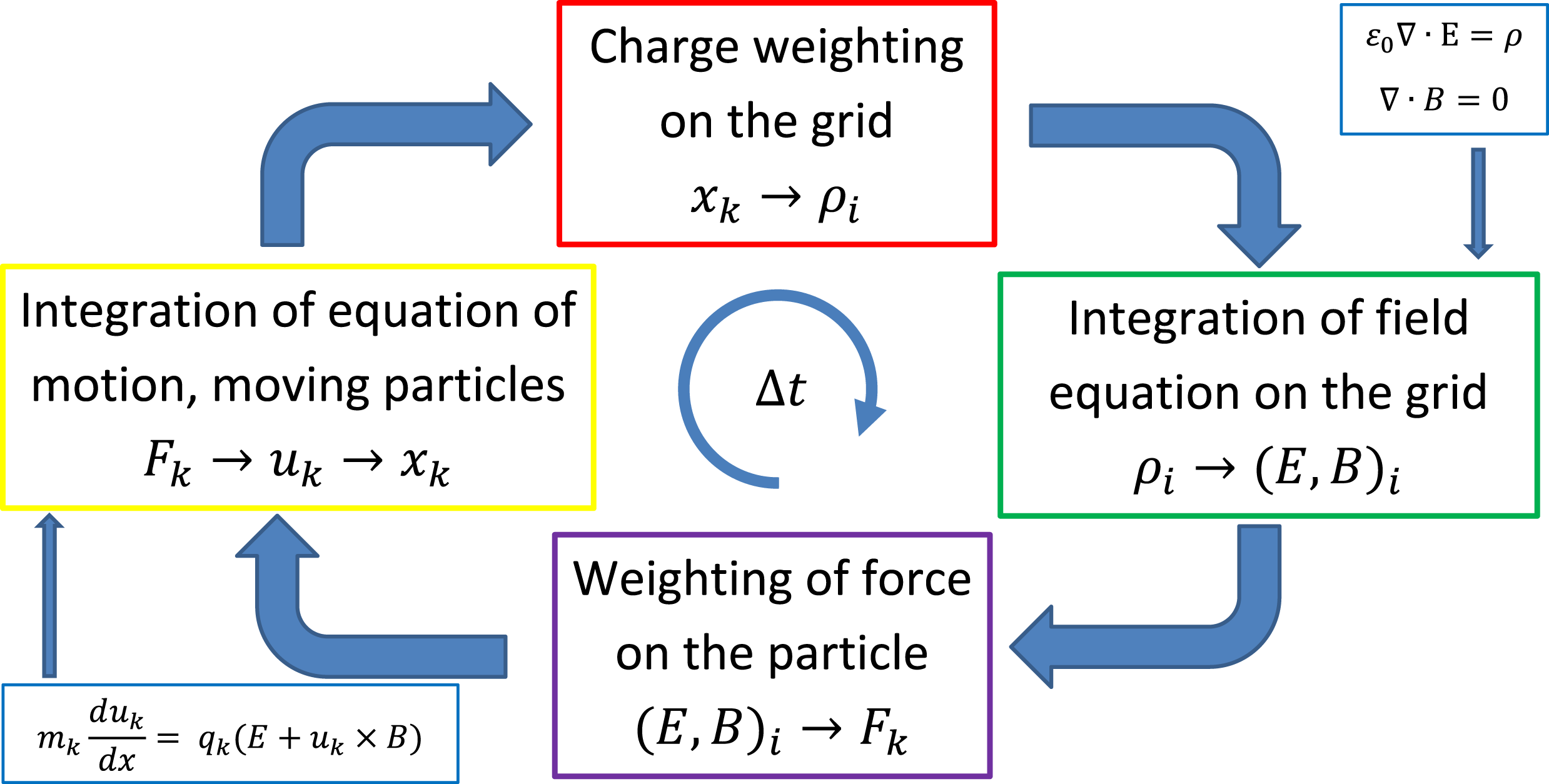
This section presents the numerical scheme implemented in EDI. EDI is an electrostatic–magnetostatic PIC code that uses an unstructured mesh of triangles. This allows us to manage arbitrary geometries. In the PIC scheme particles are defined in continuum space, while fields are defined at discrete locations in space. However, both fields and particles are defined at discrete times. In figure 1 we have proposed the general flow of the EDI code. Charge densities are calculated at grid points using a charge-conserving weighting scheme. Fields are computed using a FEM solver and are then interpolated onto particle positions with the same weighting scheme used to compute charge densities. Finally, particles are updated using a Boris leapfrog scheme and a large set of information (like particles velocities and positions) is saved.
Scheme of EDI loop. Force
 $F_{k}$
, velocity
 $u_{k}$
and position
 $x_{k}$
are referred to the particle
 $k$
. Electric filed
 $E_{i}$
, magnetic field
 $B_{i}$
and charge density
 $\unicode[STIX]{x1D70C}_{i}$
are evaluated at node
 $i$
.

2.1 The PIC method
The code simulates the evolution of charged particles due to their interaction with electromagnetic fields. The real plasma systems often contain an extremely large number of particles. In numerical simulations super-particles are used to reduce the computational cost. A super-particle (or macroparticle) is a computational particle representing many real particles, it may be millions of electrons or ions in the case of a plasma simulation (Fehske, Schneider & Weiße Reference Fehske, Schneider and Weiße2007). We will indicate with
 $p$
the number of real particles associated with a simulated super-particle. In such a way the mass and charge of the super-particle (labelled with
 $sp$
) is
 $m_{sp}=p\cdot m$
and
 $q_{sp}=p\cdot q$
where
 $q$
and
 $m$
are the charge and mass of each real particle in the system. To avoid complicated equations in EDI the number
 $p$
is fixed for all super-particles of a given species at all simulation times. The equations governing the super-particle dynamics are the equation of motion with the Lorentz force
 $$\begin{eqnarray}\displaystyle & \displaystyle m_{sp}\frac{\text{d}\boldsymbol{v}}{\text{d}t}=q_{sp}(\boldsymbol{E}+\boldsymbol{v}\times \boldsymbol{B}) & \displaystyle\end{eqnarray}$$
 $$\begin{eqnarray}\displaystyle & \displaystyle \frac{\text{d}\boldsymbol{x}}{\text{d}t}=\boldsymbol{v} & \displaystyle\end{eqnarray}$$
and Maxwell’s equations
 $$\begin{eqnarray}\frac{\text{d}\boldsymbol{E}}{\text{d}t}=c^{2}\unicode[STIX]{x1D735}\times \boldsymbol{B}-\frac{\boldsymbol{J}}{\unicode[STIX]{x1D716}_{0}}\quad \frac{d\boldsymbol{B}}{\text{d}t}=-\unicode[STIX]{x1D735}\times \boldsymbol{E}\end{eqnarray}$$
 $$\begin{eqnarray}\unicode[STIX]{x1D735}\boldsymbol{\cdot }\boldsymbol{E}=\frac{\unicode[STIX]{x1D70C}}{\unicode[STIX]{x1D716}_{0}}\quad \unicode[STIX]{x1D735}\boldsymbol{\cdot }\boldsymbol{B}=0,\end{eqnarray}$$
where
 $\boldsymbol{E}$
and
 $\boldsymbol{B}$
are the electric and magnetic fields. EDI is an electrostatic–magnetostatic code, for this reason we solve only (2.4) using a FEM formulation. For more details on the FEM implementation see § 2.5.
2.2 Spatial and temporal resolution
The mesh size is determined by the mean edge of the triangular mesh
 $a$
. In what follows we will indicate with
 $n_{e}^{0}$
the plasma electron reference density and with the superscript
 $0$
all the quantities based on it. For example
 $d_{e}^{0}=c/\unicode[STIX]{x1D714}_{\text{pe}}^{0}$
is the reference electron skin depth (
 $\unicode[STIX]{x1D714}_{\text{pe}}^{0}=\sqrt{n_{e}^{0}q_{e}^{2}/\unicode[STIX]{x1D716}_{0}m_{e}}$
is the reference plasma pulsation) and
 $\unicode[STIX]{x1D706}_{D}^{0}=\sqrt{\unicode[STIX]{x1D716}_{0}k_{B}T_{e}/n_{e}^{0}q_{e}^{2}}$
is the reference Debye length. Using these two quantities, it is possible to introduce two indicators to measure the spatial resolution of the code (Melzani et al.
Reference Melzani, Winisdoerffer, Walder, Folini, Favre, Krastanov and Messmer2013):
 $n_{a}=d_{e}^{0}/a$
and
 $n_{\unicode[STIX]{x1D706}}=\unicode[STIX]{x1D706}_{D}^{0}/a$
. A similar analysis can be performed also for the temporal scale of the code that is instead defined starting from the global simulation time step
 $\unicode[STIX]{x0394}t$
. In fact, if we define with
 $T_{pe}^{0}=2\unicode[STIX]{x03C0}/\unicode[STIX]{x1D714}_{pe}^{0}$
the reference electron plasma period, then the temporal resolution of the code is given by the quantity
 $n_{t}=T_{pe}^{0}/\unicode[STIX]{x0394}t$
.
2.3 The mesh management
The code uses an unstructured mesh of triangles. The Delaunay mesh is built using an open-source software called Gmsh (http://gmsh.info) (Geuzaine & Remacle Reference Geuzaine and Remacle2009). Gmsh is a free 2-D/3-D finite element grid generator with a build-in computer-aided drafting (CAD) engine and post-processor. The final
 $.msh$
ASCII output file contains the mesh nodes, the elements, the region names and so on. In EDI we have included a parser able to import the
 $.msh$
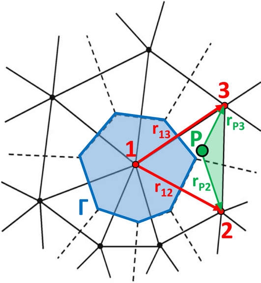
file and to construct the connectivity table of the mesh. This table is constructed by progressively adding mesh elements starting at the boundaries. This iteration results in a propagation of a front (internal boundary) between the meshed and the unmeshed region. For each node the parser computes also a list of the barycentres of the triangles that include the node. This list is then used to compute the area
 $\unicode[STIX]{x1D6E4}$
of the Voronoy cell associated with the node (see figure 2). Each area is computed using an open source software called Qhull (http://www.qhull.org) (Barber et al.
Reference Barber, Dobkin, Dobkin and Huhdanpaa1996).
The parameter
 $\unicode[STIX]{x1D6E4}$
is the area of the Voronoy cell associated with node 1. The particle
 $P$
is located inside the triangular mesh element of vertices 1, 2 and 3. The vectors
 $\boldsymbol{r}_{\mathbf{12}}$
and
 $\boldsymbol{r}_{\mathbf{13}}$
are employed to calculate the surface of the triangular mesh element
 $\unicode[STIX]{x1D6FA}_{123}$
, while the vectors
 $\boldsymbol{r}_{\boldsymbol{P}\pmb{{\it 2}}}$
and
 $\boldsymbol{r}_{\boldsymbol{P}\pmb{{\it 3}}}$
are used for the surface
 $\unicode[STIX]{x1D6FA}_{P23}$
(depicted in green), see (2.8). Figure from Spirkin (Reference Spirkin2006).

2.4 Weighting scheme (charge deposition)
In § 2.1 we have described the concept of super-particle used in PIC simulations. In order to compute the nodal charge density it is necessary to introduce a function designated as the particle shape or a weighting function. We have followed the approach proposed by Hockney & Eastwood (Reference Hockney and Eastwood1988), with particular attention paid to the analysis performed by Spirkin (Reference Spirkin2006), who describes this process by using a function that will be denoted in the following with
 $W$
. The area of overlap between the particle shape and the grid cell determines the charge assigned to the grid point. We will call
 $W_{I}(\boldsymbol{r}_{\boldsymbol{P}})$
the fraction of a charge from a particle
 $P$
located at
 $\boldsymbol{r}_{\boldsymbol{P}}=(x_{p},y_{p})$
assigned to the grid point
 $I$
located at
 $\boldsymbol{r}_{\boldsymbol{I}}=(x_{I},y_{I})$
. Charge conservation requires that
 $$\begin{eqnarray}\mathop{\sum }_{I=1}^{M}W_{I}(\boldsymbol{r}_{\boldsymbol{p}})=1,\end{eqnarray}$$
where the sum is taken over
 $M$
nodes used to distribute the charge close to the particle position. If we consider a 2-D domain discretized by an unstructured Delauney grid, each triangular cell is formed by three nodes. Consider now a particle
 $P$
located inside the element identified by nodes 1, 2 and 3 whose positions are respectively
 $\boldsymbol{r}_{\mathbf{1}}=(x_{1},y_{1})$
,
 $\boldsymbol{r}_{\mathbf{2}}=(x_{2},y_{2})$
and
 $\boldsymbol{r}_{\mathbf{3}}=(x_{3},y_{3})$
(see figure 2). We assign the charge of the particle
 $P$
to these three nodes. In this case, charge conservation requires that
 $$\begin{eqnarray}\mathop{\sum }_{I=1}^{3}W_{I}(\boldsymbol{r}_{\boldsymbol{p}})=1,\end{eqnarray}$$
where
 $W_{I}$
is defined as
 $$\begin{eqnarray}\left.\begin{array}{@{}c@{}}W_{1}={\displaystyle \frac{\unicode[STIX]{x1D6FA}_{P23}}{\unicode[STIX]{x1D6FA}_{123}}}\\ W_{2}={\displaystyle \frac{\unicode[STIX]{x1D6FA}_{P31}}{\unicode[STIX]{x1D6FA}_{123}}}\\ W_{3}={\displaystyle \frac{\unicode[STIX]{x1D6FA}_{P12}}{\unicode[STIX]{x1D6FA}_{123}}}.\end{array}\right\}\end{eqnarray}$$
In particular
 $$\begin{eqnarray}\left.\begin{array}{@{}c@{}}\unicode[STIX]{x1D6FA}_{123}={\textstyle \frac{1}{2}}|\boldsymbol{r}_{\mathbf{13}}\times \boldsymbol{r}_{\mathbf{23}}|\\ \unicode[STIX]{x1D6FA}_{P23}={\textstyle \frac{1}{2}}|\boldsymbol{r}_{\mathbf{P2}}\times \boldsymbol{r}_{\mathbf{P3}}|,\end{array}\right\}\end{eqnarray}$$
where
 $\boldsymbol{r}_{\boldsymbol{P}\pmb{{\it 2}}}=\boldsymbol{r}_{\mathbf{2}}-\boldsymbol{r}_{\boldsymbol{P}}$
,
 $\boldsymbol{r}_{\boldsymbol{P}\pmb{{\it 3}}}=\boldsymbol{r}_{\mathbf{3}}-\boldsymbol{r}_{\boldsymbol{P}}$
,
 $\boldsymbol{r}_{\mathbf{12}}=\boldsymbol{r}_{\mathbf{2}}-\boldsymbol{r}_{\mathbf{1}}$
and
 $\boldsymbol{r}_{\mathbf{13}}=\boldsymbol{r}_{\mathbf{3}}-\boldsymbol{r}_{\mathbf{1}}$
. It is worth recalling that: (i)
 $\unicode[STIX]{x1D6FA}_{123}$
is equal to the surface of the triangular mesh element, and (ii)
 $\unicode[STIX]{x1D6FA}_{P23}$
to the surface delimited by the particle
 $P$
and the nodes 2 and 3 (depicted in green in figure 2). The quantities
 $\unicode[STIX]{x1D6FA}_{P31}$
and
 $\unicode[STIX]{x1D6FA}_{P12}$
are computed in a similar manner. The number density and charge density due to
 $N_{s}$
particles of species
 $s$
(with charge
 $q_{s}$
) at a fixed node (e.g. nude 1) with coordinates
 $\boldsymbol{r}_{\mathbf{1}}=(x_{1},y_{1})$
can be evaluated as
 $$\begin{eqnarray}\displaystyle & \displaystyle n_{s}(x_{1},y_{1})=\frac{1}{\unicode[STIX]{x1D6E4}}\mathop{\sum }_{p=1}^{N_{s}}W_{1}(x_{p},y_{p}) & \displaystyle\end{eqnarray}$$
 $$\begin{eqnarray}\displaystyle & \displaystyle \unicode[STIX]{x1D70C}_{s}(x_{1},y_{1})=\frac{q_{s}}{\unicode[STIX]{x1D6E4}}\mathop{\sum }_{p=1}^{N_{s}}W_{1}(x_{p},y_{p}), & \displaystyle\end{eqnarray}$$
where
 $\unicode[STIX]{x1D6E4}$
is the area of the Voronoy cell where the particle is located (see figure 2).
Finally, it is worth recalling that the weighting scheme adopted does not require particular adjustments if the mesh is non-uniform. In fact each particle deposits charge only on the nodes of the element in which it is located. This approach is physically meaningful if the size of the mesh element is of the order of the Debye length in all of the domain; namely, the finer mesh where the plasma is denser (Birdsall & Langdon Reference Birdsall and Langdon2004).
2.5 The field FEM formulation
In EDI the fields are computed, at each time step, using a FEM formulation. EDI is an electrostatic–magnetostatic code, namely only equations (2.4) are solved among Maxwell’s set. In order to define a FEM approximation of equations (2.4), a weak formulation has been adopted (Bossavit Reference Bossavit1998; Polycarpou Reference Polycarpou2005). We assume that the problem is defined in a region
 $\unicode[STIX]{x1D6FA}$
which is an open, polygonal and simply connected set while
 $\unicode[STIX]{x2202}\unicode[STIX]{x1D6FA}$
denotes its frontier (Pinto et al.
Reference Pinto, Jund, Salmon, Sonnendrücker and Lorraine2008):
 $$\begin{eqnarray}\left.\begin{array}{@{}c@{}}H_{1}(\unicode[STIX]{x1D6FA})=\{v\in L^{2}(\unicode[STIX]{x1D6FA}):\unicode[STIX]{x1D735}v\in \boldsymbol{L}^{2}(\unicode[STIX]{x1D6FA},\mathbb{R}^{n})\}\\ H_{0}^{1}(\unicode[STIX]{x1D6FA})=\{v\in H_{1}(\unicode[STIX]{x1D6FA}):v|_{\unicode[STIX]{x2202}\unicode[STIX]{x1D6FA}}=0\}\end{array}\right\}\end{eqnarray}$$
for more details, see Girault & Raviart (Reference Girault and Raviart2012). The electrostatic problem has been formulated in terms of Poisson’s equation
 $$\begin{eqnarray}\unicode[STIX]{x1D735}\boldsymbol{\cdot }\boldsymbol{E}=\frac{\unicode[STIX]{x1D70C}}{\unicode[STIX]{x1D716}_{0}}\rightarrow \unicode[STIX]{x1D735}\boldsymbol{\cdot }(\unicode[STIX]{x1D716}_{0}\unicode[STIX]{x1D735}\unicode[STIX]{x1D719})=-\unicode[STIX]{x1D70C},\end{eqnarray}$$
where
 $\unicode[STIX]{x1D719}$
is the unknown electrostatic potential. The weak formulation reads (Bossavit Reference Bossavit1998; Pinto et al.
Reference Pinto, Jund, Salmon, Sonnendrücker and Lorraine2008)
 $$\begin{eqnarray}\int _{\unicode[STIX]{x1D6FA}}\unicode[STIX]{x1D716}_{0}\unicode[STIX]{x1D735}\unicode[STIX]{x1D719}\boldsymbol{\cdot }\unicode[STIX]{x1D735}\unicode[STIX]{x1D719}^{\prime }\,\text{d}\unicode[STIX]{x1D6FA}=\int _{\unicode[STIX]{x1D6FA}}\unicode[STIX]{x1D70C}\unicode[STIX]{x1D719}^{\prime }\,\text{d}\unicode[STIX]{x1D6FA}\quad \forall \unicode[STIX]{x1D719}^{\prime }\in H_{0}^{1}(\unicode[STIX]{x1D6FA}),\end{eqnarray}$$
where
 $\unicode[STIX]{x1D719}^{\prime }$
is a scalar test function. For the magnetostatic problem, we have assumed that the static magnetic fields is generated by magnets. Therefore we have solved the following problem using a
 $\boldsymbol{H}$
conforming formulation (Dular et al.
Reference Dular, Henrotte, Robert, Genon and Legros1997)
 $$\begin{eqnarray}\unicode[STIX]{x1D735}\boldsymbol{\cdot }\boldsymbol{B}=0.\end{eqnarray}$$
The weak formulation reads (Dular & Geuzaine Reference Dular and Geuzaine2016)
 $$\begin{eqnarray}\int _{\unicode[STIX]{x1D6FA}}\unicode[STIX]{x1D707}(\boldsymbol{H}_{\boldsymbol{s}}-\unicode[STIX]{x1D735}\unicode[STIX]{x1D701})\boldsymbol{\cdot }\unicode[STIX]{x1D735}\unicode[STIX]{x1D719}^{\prime }\,\text{d}\unicode[STIX]{x1D6FA}=0\quad \forall \unicode[STIX]{x1D719}^{\prime }\in H_{0}^{1}(\unicode[STIX]{x1D6FA}),\end{eqnarray}$$
where
 $\boldsymbol{H}_{\boldsymbol{s}}$
is the source field and
 $\unicode[STIX]{x1D701}$
is the scalar unknown potential for which
 $\boldsymbol{H}=-\unicode[STIX]{x1D735}\unicode[STIX]{x1D701}$
. If we consider a permanent magnet we can assume that the magnetic field has the same value in all the internal points of the magnet so we can write
 $$\begin{eqnarray}\boldsymbol{H}_{\boldsymbol{s}}=\boldsymbol{H}_{\boldsymbol{c}}(\boldsymbol{x})\quad \forall \boldsymbol{x}\in \text{Magnets},\end{eqnarray}$$
where
 $\boldsymbol{H}_{\boldsymbol{c}}$
is the coercive magnetic field of the magnet assumed fixed and measured in
 $\text{A}~\text{m}^{-1}$
. Equations (2.13)–(2.15) are the weak formulation of (2.4) and can be solved with any FEM solver once appropriate boundary conditions are defined (Dirichlet in our case). In the current implementation of EDI, we managed to use the open source software GetDP (a ‘General environment for the treatment of Discrete Problems’) (Geuzaine Reference Geuzaine2007). GetDP is a well-established scientific software environment for the numerical solution of integro-differential equations. In particular, its capability in solving electro-magnetic (EM) problems has been proven both in the industrial (Trophime et al.
Reference Trophime, Egorov, Debray, Joss and Aubert2002; Sabariego et al.
Reference Sabariego, Gyselinck, Dular, De Coster, Henrotte and Hameyer2004) and the plasma physics (Damyanova, Sabchevski & Zhelyazkov Reference Damyanova, Sabchevski and Zhelyazkov2010) fields. In the current implementation, GetDP has been properly modified in order to accept EDI input parameters (e.g. nodal plasma density and electron temperature) and to solve the electrostatic/magnetostatic problem. The final GetDP outputs are the
 $\boldsymbol{E}$
and
 $\boldsymbol{B}$
fields at EDI nodes. From a numerical standpoint, the stationary equations (2.13)–(2.15) are solved separately at each time step in order to grasp respectively the
 $\unicode[STIX]{x1D719}$
and
 $\unicode[STIX]{x1D701}$
potentials. On the triangular elements of the mesh, the potential field can be represented as a third-order polynomial of the form (Dular & Geuzaine Reference Dular and Geuzaine2016)
 $$\begin{eqnarray}\unicode[STIX]{x1D719}(\boldsymbol{x})=\mathop{\sum }_{j=1}^{3}\unicode[STIX]{x1D719}_{j}L_{j}(\boldsymbol{x}),\end{eqnarray}$$
where
 $\boldsymbol{x}$
is a generic position,
 $\unicode[STIX]{x1D719}_{j}$
is the scalar potential in the node
 $j$
of a specific triangular element and
 $L_{j}$
is the basis function (specifically, a Lagrange polynomial) associated with the same node. An equation similar to (2.17), holds true also for the
 $\unicode[STIX]{x1D701}$
potential. In particular, in the GetDP environment, equation (2.17) is implemented setting the FunctionSpace as 0-form type and the basis function as BF-Node (Dular & Geuzaine Reference Dular and Geuzaine2016). Once the basis functions are defined (see (2.17)), the governing equations expressed in the weak form (see (2.13)–(2.15)) can be reduced to algebraic linear systems thanks to the Galerkin method (Quarteroni, Sacco & Saleri Reference Quarteroni, Sacco and Saleri2010). The latter is implemented in GetDP setting the problem Formulation as FemEquation (Dular & Geuzaine Reference Dular and Geuzaine2016). Finally, the two resulting linear systems are solved with the lower-upper (LU) decomposition algorithm implemented in the PETSc library (Balay Reference Balay2001).
2.6 Particle initialization
In EDI, particles of each species can be initially loaded into the whole simulation domain or into a fixed region. The region in which particles are loaded will be called in the following the ‘loading region’. If the mesh and the plasma are uniform, each particle to be loaded is attributed to a randomly chosen triangle. Otherwise, the same procedure is repeated associating different probabilities to each mesh element depending on: (i) the density imposed at its barycentre, (ii) its surface. Anyway, let us assume that a particle has to be loaded on the triangle whose vertices are
 $\boldsymbol{A}=(x_{A},y_{A})$
,
 $\boldsymbol{B}=(x_{B},y_{B})$
and
 $\boldsymbol{C}=(x_{C},y_{C})$
. We position the particle at a point
 $\boldsymbol{P}=(x_{P},y_{P})$
on the triangle surface by generating two random numbers
 $r_{1}$
and
 $r_{2}$
between 0 and 1 and solving the following equation (Osada et al.
Reference Osada, Funkhouser, Chazelle and Dobkin2002)
 $$\begin{eqnarray}\boldsymbol{P}=(1-\sqrt{r_{1}})\boldsymbol{A}+\sqrt{r_{1}}(1-r_{2})\boldsymbol{B}+\sqrt{r_{1}}r_{2}\boldsymbol{C}.\end{eqnarray}$$
Equation (2.18) gives a uniform random point distribution with respect to the surface of the chosen triangle.
In addition, several momentum and energy distributions are available that can be used to initialize the energy and the momentum of the particles in the loading region. In this paper we have used two types of loading distribution. A Maxwell–Boltzmann distribution in energy
 $$\begin{eqnarray}f(x)=\frac{1}{\sqrt{2\unicode[STIX]{x03C0}}\unicode[STIX]{x1D70E}}\text{e}^{-(x-E)^{2}/2\unicode[STIX]{x1D70E}^{2}},\end{eqnarray}$$
with expectation value
 $E$
and variance
 $\unicode[STIX]{x1D70E}^{2}$
. A convolution of two Gaussian distributions (Hu Reference Hu2016) along the
 $v_{x}$
velocity component for the two stream instability test (§ 3.3)
 $$\begin{eqnarray}f(v_{x},v_{y})=\frac{1}{2}\left(\frac{1}{\sqrt{2\unicode[STIX]{x03C0}}\unicode[STIX]{x1D70E}}\text{e}^{-(v_{x}+v_{D})^{2}/2\unicode[STIX]{x1D70E}^{2}}+\frac{1}{\sqrt{2\unicode[STIX]{x03C0}}\unicode[STIX]{x1D70E}}\text{e}^{-(v_{x}-v_{D})^{2}/2\unicode[STIX]{x1D70E}^{2}}\right)\unicode[STIX]{x1D6FF}(v_{y}),\end{eqnarray}$$
with expectation value for each Gaussian function equal to
 $\pm v_{D}$
and variance
 $\unicode[STIX]{x1D70E}^{2}$
;
 $\unicode[STIX]{x1D6FF}(x)$
is the Dirac delta function, defined by
 $\unicode[STIX]{x1D6FF}(x)=\infty$
for
 $x=0$
and
 $\int _{-\infty }^{\infty }\unicode[STIX]{x1D6FF}(x)\,\text{d}x=1$
. Usually
 $\unicode[STIX]{x1D70E}$
matches with
 $v_{th}$
, the thermal velocity of each species. For the two stream instability test
 $\unicode[STIX]{x1D70E}\rightarrow 0$
. From this it follows that (2.20) can be rewritten as
 $$\begin{eqnarray}f(v_{x},v_{y})={\textstyle \frac{1}{2}}[\unicode[STIX]{x1D6FF}(v_{x}+v_{D})+\unicode[STIX]{x1D6FF}(v_{x}-v_{D})]\unicode[STIX]{x1D6FF}(v_{y}).\end{eqnarray}$$
In the present code, in order to generate particles according to the distribution functions described in (2.19) and (2.20) we used the method called inversion of cumulative distribution functions. See D’Agostini (Reference D’Agostini2003) for more details.
2.7 Particle updating
The particle motion is described in (2.1) and (2.2). Equation (2.2) can be discretized in three dimensions after Umeda (Reference Umeda2003) and Umeda et al. (Reference Umeda, Omura, Tominaga and Matsumoto2003) as
 $$\begin{eqnarray}\displaystyle & \displaystyle x^{t+\unicode[STIX]{x0394}t}=x^{t}+v_{x}^{t+(\unicode[STIX]{x0394}t/2)}\unicode[STIX]{x0394}t & \displaystyle\end{eqnarray}$$
 $$\begin{eqnarray}\displaystyle & \displaystyle y^{t+\unicode[STIX]{x0394}t}=y^{t}+v_{y}^{t+(\unicode[STIX]{x0394}t/2)}\unicode[STIX]{x0394}t & \displaystyle\end{eqnarray}$$
 $$\begin{eqnarray}\displaystyle & \displaystyle z^{t+\unicode[STIX]{x0394}t}=z^{t}+v_{z}^{t+(\unicode[STIX]{x0394}t/2)}\unicode[STIX]{x0394}t & \displaystyle\end{eqnarray}$$
and (2.1) as
 $$\begin{eqnarray}\boldsymbol{v}^{t+(\unicode[STIX]{x0394}t/2)}=\boldsymbol{v}^{t-(\unicode[STIX]{x0394}t/2)}+\unicode[STIX]{x0394}t\frac{q_{sp}}{m_{sp}}(\boldsymbol{E}^{t}+\boldsymbol{v}^{t}\times \boldsymbol{B}^{t}).\end{eqnarray}$$
Since
 $\boldsymbol{v}^{t}$
is not known a priori, equation (2.25) can be rewritten as
 $$\begin{eqnarray}\boldsymbol{v}^{t+(\unicode[STIX]{x0394}t/2)}=\boldsymbol{v}^{t-(\unicode[STIX]{x0394}t/2)}+\unicode[STIX]{x0394}t\frac{q_{sp}}{m_{sp}}\left(\boldsymbol{E}^{t}+\frac{\boldsymbol{v}^{t+(\unicode[STIX]{x0394}t/2)}+\boldsymbol{v}^{t-(\unicode[STIX]{x0394}t/2)}}{2}\times \boldsymbol{B}^{t}\right).\end{eqnarray}$$
Using (2.26) and following the approach proposed in Birdsall & Langdon (Reference Birdsall and Langdon2004) and Hockney & Eastwood (Reference Hockney and Eastwood1988), it is possible to compute
 $\boldsymbol{v}^{t+(\unicode[STIX]{x0394}t/2)}$
using a four step computation usually known as the ‘Buneman–Boris method’. At the first time step the velocity is pushed back to the time
 $t-\unicode[STIX]{x0394}t/2$
. In addition to the just exposed algorithm, in EDI we have introduced other integration schemes, like the relativistic Vay algorithm (Vay Reference Vay2008). However in the simulation used to benchmark the code we have used only the just exposed integrator, so that we will not discuss the other integration schemes.
2.8 Particle tracking
After each time step, particles are tracked in the unstructured triangle grid using an efficient and robust particle-localization algorithm. Given the previous particle position and the cell containing that position, the algorithm determines the cell which contains a nearby position. The algorithm is based on tracking a particle along its trajectory by computing the intersections of the trajectory and the cell faces and it is a modified version of the one proposed in Haselbacher, Najjar & Ferry (Reference Haselbacher, Najjar and Ferry2007).
2.9 Fields and particle boundaries
In EDI we have introduced different fields and particles boundary conditions. For the particles we have introduced conductive and reflective boundaries. A secondary boundary electron emission subroutine is now being developed using the approach proposed in Seiler (Reference Seiler1983) and Taccogna, Longo & Capitelli (Reference Taccogna, Longo and Capitelli2004) and it will be added to the particle boundary management. Also, fields have different types of boundaries. These could be periodic (field quantities at one boundary are equal to those at the other boundary), Dirichlet or Neumann boundary conditions depending on the material types and on the chosen FEM implementation (Bossavit Reference Bossavit1998).
2.10 The main loop
In EDI we have defined a full integer time step
 $n\unicode[STIX]{x0394}t$
and a half-integer time step
 $(n+1/2)\unicode[STIX]{x0394}t$
. As already stated, fields are computed using a FEM formulation, for this reason these are known at integer time steps i.e.
 $\boldsymbol{E}^{t}$
and
 $\boldsymbol{B}^{t}\quad \forall t$
. The particle position
 $\boldsymbol{r}$
is known at the full integer time step, and velocities
 $\boldsymbol{v}$
at the half-integer time step. As initial condition, we provide
 $\boldsymbol{r}^{\boldsymbol{t}}$
,
 $\boldsymbol{v}^{t-(\unicode[STIX]{x0394}t/2)}$
,
 $\boldsymbol{E}^{t}$
,
 $\boldsymbol{B}^{t}$
. The structure of the main loop is the following:
(i) update particle velocity from
 $t-\unicode[STIX]{x0394}t/2$
to
$t+\unicode[STIX]{x0394}t/2$
:
$\boldsymbol{v}^{t+(\unicode[STIX]{x0394}t/2)}$
;
(ii) update the position
$\boldsymbol{r}$
from
$t$
to
$t+\unicode[STIX]{x0394}t$
using
$\boldsymbol{v}^{t+(\unicode[STIX]{x0394}t/2)}$
;(iii) particle tracking;
(iv) boundary management for particles;
(v) test exit condition;
(vi) particle source;
(vii) weighting scheme (charge deposition);
(viii) advance electric and magnetic fields from
$t$
to
$t+\unicode[STIX]{x0394}t$
with the FEM solver.


2.11 Particle source
At the end of each main loop of the code (steps 1–6 in the list of § 2.10), if needed, a particle source inserts a fixed number of particles into the system. These particles can be introduced into a fixed simulation region or into the whole simulation domain according to the requirements. The particle source inserts the particles using the same spatial and energy distribution functions already presented in § 2.6.
2.12 Time loop termination
The main time loop is terminated once a user-specified exit condition is satisfied. EDI supports two conditions (Brieda Reference Brieda2005):
(i) maximum number of time steps;
(ii) steady state.
A simulation is assumed to be at the steady state if the number of particles leaving through the external boundaries matches the number of new particles introduced into the system by the source. This condition shall be met for a sufficiently high number of time steps (
 $m$
) in order to avoid a ‘false-positive’ induced by PIC noise. In particular, the steady-state condition is implemented by requiring that:
 $$\begin{eqnarray}\frac{1}{m+1}\mathop{\sum }_{k=h-m}^{h}\frac{|N_{sp}^{k}-N_{sp}^{k-1}|}{N_{sp}^{k}}<\unicode[STIX]{x1D708},\end{eqnarray}$$
where
 $\unicode[STIX]{x1D708}$
is a user defined number that represents a steady-state condition (usually
 $\unicode[STIX]{x1D708}\sim 10^{-4}$
),
 $N_{sp}^{k}$
is the number of super-particles in the system at the time step
 $k$
, and
 $h$
is the current time step. As a rule of thumb, we can assume
 $m\sim 50$
.
2.13 Output and data analysis
At the end of each time step, simulation results are saved in different file formats. EDI provides two types of output file:
 $.dat$
files, with particle positions and velocities, and/or
 $.pos$
files (Gmsh format). The latter is useful to visualize, using Gmsh, the evolution of quantities of interest like charge density. A DUMP file is also provided. This DUMP file produces a binary file that is used to save, at a user predefined time step, the configuration of the electromagnetic fields and/or particles velocities and positions. A parser is also provided to import the DUMP file and to load it as initial condition. These data can be used to start the simulation with a prefixed configuration i.e. a predefined configuration of fields and particles.
3 Code validation
In this section, we will discuss three tests performed to benchmark the new EDI PIC code. The first test (§ 3.1) is devoted to checking the correct integration of GetDP on EDI. The magnetostatic field computed by EDI (more precisely by GetDP integrated on EDI) has been compared against the results of an external solver, namely the open source code FEMM (Meeker Reference Meeker2014). It is worth highlighting that the aim of this test is not to evaluate the numerical model implemented on GetDP, but rather it is intended to validate the information exchange (namely, values of the EM fields at nodes) between GetDP and EDI. Subsequently we have analysed some classical plasma models to prove how EDI is able to handle different physical problems and to reproduce precise analytical results. The second test (§ 3.2) consists of studying the oscillation modes of a cold plasma by means of a FT analysis. The third and last tests (§ 3.3) consist in analysing the two stream instability formation, paying particular attention to the linear stage of this instability.
3.1 GetDP integration on EDI
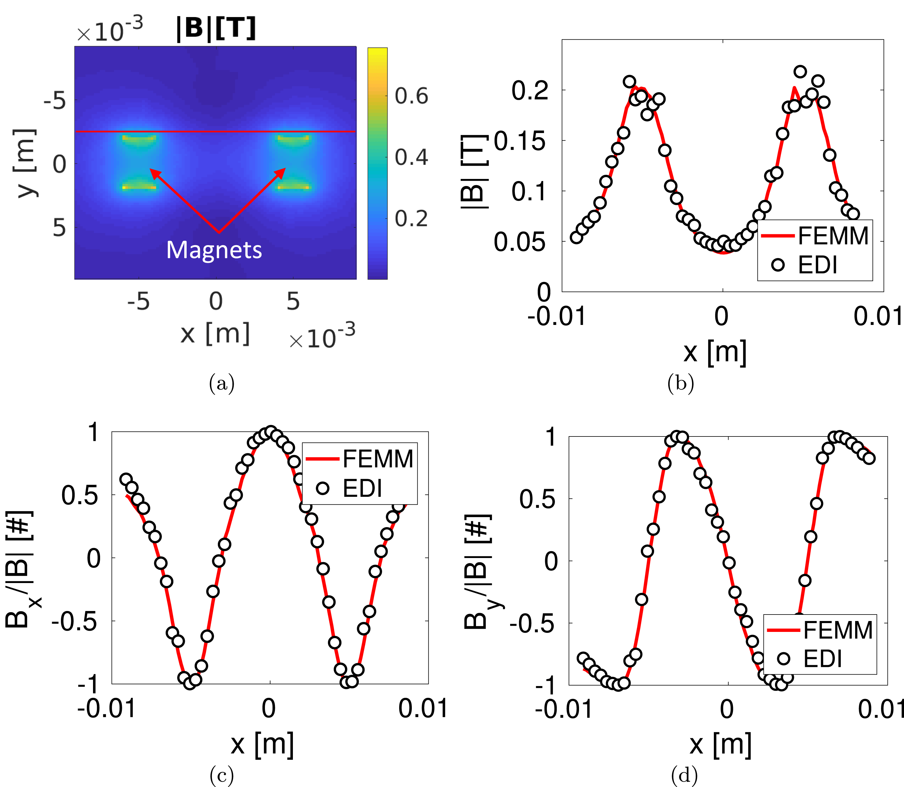
Comparison between the magnetic fields
 $\boldsymbol{B}$
computed by EDI and FEMM: (a) intensity of the reference field computed with FEMM; (b) comparison between
 $|\boldsymbol{B}|$
; (c) comparison between
 $B_{x}/|B|$
; (d) comparison between
 $B_{y}/|B|$
. The comparisons are performed along
 $y=-2.5~\text{mm}$
(see red line in a).

As previously stated, in EDI the EM fields are calculated by the external solver GetDP. The latter has been properly modified in respect of classical formulations (e.g. Trophime et al.
Reference Trophime, Egorov, Debray, Joss and Aubert2002; Sabariego et al.
Reference Sabariego, Gyselinck, Dular, De Coster, Henrotte and Hameyer2004) in order to provide to EDI the EM fields at the mesh nodes. In order to check (i) the implementation of (2.13)–(2.15) on GetDP, and (ii) the correct integration of GetDP on EDI, the results of GetDP-EDI have been benchmarked against FEMM (Meeker Reference Meeker2014). In particular, the two solvers have been exploited to calculate the magnetostatic field generated by two permanent magnets made of SmCo immersed in a vacuum region (magnetic permeability outside the magnets equal to the vacuum permittivity
 $\unicode[STIX]{x1D707}_{0}$
) and in the absence of plasma. The benchmark magnetic field computed with FEMM is reproduced in figure 3(a). We have defined a line along which we have compared the magnetic field calculated with the two solvers (see the red line in figure 3
a at
 $y=-2.5~\text{mm}$
). The comparison is reproduced in figure 3(b–d). The greater noise of the EDI curve in the position closer to the magnets is mainly due to the interpolation that was used to compute the magnetic field at the same mesh points used by FEMM. Nonetheless, the agreement between the two codes is satisfactory and we can conclude that the implementation of the equations in GetDP, and in particular their integration in EDI, are correct.
It is worth underlining that the FEM formulation implemented on GetDP has been evaluated with other tests where: (i) the capability of EDI in reproducing analytical results has been tested, and in turn the accuracy of the EM solver can be checked (see §§ 3.2 and 3.3), and (ii) the computational time required by each operation of EDI, along with how it scales with the size of the mesh and time step, has been investigated in a convergence study (see § 3.3).
3.2 Oscillation mode analysis
The second test consists of simulating the oscillation modes of a cold plasma. In particular we have analysed only the evolution of electrons in a fixed background of ions. Generally speaking, the wave spectrum can be analysed by means of the FT of the velocity field, in particular
 $$\begin{eqnarray}F_{x}(\boldsymbol{k},\unicode[STIX]{x1D714})=\iint v_{x}(\boldsymbol{x},t)\text{e}^{-\text{i}(\boldsymbol{k}\boldsymbol{\cdot }\boldsymbol{x}+\unicode[STIX]{x1D714}t)}\,\text{d}V\,\text{d}t,\end{eqnarray}$$
where
 $F_{x}$
is the FT of the component along the
 $x$
axis of velocity (
 $v_{x}$
),
 $\boldsymbol{k}$
is the wavevector (Inan & Gołkowski Reference Inan and Gołkowski2010),
 $\boldsymbol{x}$
is a generic position vector in the domain,
 $\unicode[STIX]{x1D714}$
is the frequency,
 $t$
is the time and
 $\text{i}$
is an imaginary constant. Similarly,
 $F_{y}$
is defined as the FT of the component along the
 $y$
axis of the velocity (
 $v_{y}$
). To keep the analysis lucid, we have studied only the frequency modes of zero wavevector,
 $\boldsymbol{k}=0$
(Melzani et al.
Reference Melzani, Winisdoerffer, Walder, Folini, Favre, Krastanov and Messmer2013). In such a way, equation (3.1) reduces to
 $$\begin{eqnarray}F_{x}(\mathbf{0},\unicode[STIX]{x1D714})=\int \left(\int v_{x}(\boldsymbol{x},t)\,\text{d}V\right)\text{e}^{-\text{i}\unicode[STIX]{x1D714}t}\,\text{d}t=\int q_{x}(t)\text{e}^{-\text{i}\unicode[STIX]{x1D714}t}\,\text{d}t,\end{eqnarray}$$
where
 $q_{x}$
is the volume integral of
 $v_{x}$
. Similarly,
 $q_{y}$
can be defined with respect to
 $v_{y}$
. Therefore, equation (3.2) can be discretized by means of a fast Fourier transform (FFT) as (Melzani et al.
Reference Melzani, Winisdoerffer, Walder, Folini, Favre, Krastanov and Messmer2013)
 $$\begin{eqnarray}F_{x}(\unicode[STIX]{x1D714})\approx \mathop{\sum }_{k=1}^{N_{t}}\left(\mathop{\sum }_{i=1}^{N_{sp}}v_{ix}(t_{k})\right)\text{e}^{-\text{i}\unicode[STIX]{x1D714}t_{k}},\end{eqnarray}$$
where
 $N_{t}$
is the total number of integration time steps,
 $t_{k}$
is the time at the time step
 $k$
,
 $N_{sp}$
is the number of electron super-particles and
 $v_{ix}$
is the component along the
 $x$
axis of the velocity of the super-particle
 $i$
. In particular, also
 $F_{y}$
can be discretized in the same manner as described in (3.3). It is worth highlighting that in (3.3), the
 $q_{x}$
term has been approximated as (Melzani et al.
Reference Melzani, Winisdoerffer, Walder, Folini, Favre, Krastanov and Messmer2013)
 $$\begin{eqnarray}q_{x}\approx \mathop{\sum }_{i=1}^{N_{sp}}v_{ix}\end{eqnarray}$$
provided that: (i) with the weighting scheme adopted (see § 2.4), each super-particle is assumed to have the size of the triangular mesh element inside which it is located (Spirkin Reference Spirkin2006), and (ii) for this test, we have adopted a uniform mesh. Simulation parameters (see § 2.2) have been chosen in accordance with table 1. The simulation domain is a square box of side
 $L=2~\text{cm}$
aligned with the
 $x$
and
 $y$
axes of a Cartesian reference system. Particles are inserted into the domain with the distribution function described in (2.19). Reflecting boundaries were chosen for particles.
We have analysed the electrostatic electron fluctuations with and without the presence of an external background magnetic field
 $\boldsymbol{B}_{\mathbf{0}}$
perpendicular to the simulation domain, namely aligned along the
 $z$
axis. In the absence of a background magnetic field (see § 3.2.1), electrons perform Langmuir oscillations with a characteristic frequency equal to the plasma frequency
 $\unicode[STIX]{x1D714}_{pe}$
. Provided that these oscillations involve the creation of electric fields by local charge imbalance, this first analysis investigates the capability of the code to reproduce the field propagation, as well as particle motion (Melzani et al.
Reference Melzani, Winisdoerffer, Walder, Folini, Favre, Krastanov and Messmer2013). When the magnetic field is present (see § 3.2.2) and when this field is high enough, the Langmuir motion is fully covered by the Larmor motion in a plane perpendicular to
 $\boldsymbol{B}_{\mathbf{0}}$
with a characteristic frequency equal to
 $\unicode[STIX]{x1D714}_{c}=q_{e}|\boldsymbol{B}_{\mathbf{0}}|/m_{e}$
. This example then probes the accuracy of the particle motion integrator (Melzani et al.
Reference Melzani, Winisdoerffer, Walder, Folini, Favre, Krastanov and Messmer2013). Moreover, in an intermediate regime, electrons oscillate with a characteristic frequency equal to the upper hybrid frequency
 $\unicode[STIX]{x1D714}_{h}^{2}=\unicode[STIX]{x1D714}_{pe}^{2}+\unicode[STIX]{x1D714}_{c}^{2}$
.
Simulation parameters (see § 2.2) adopted during the oscillation mode analysis.

3.2.1 Absence of a background magnetic field
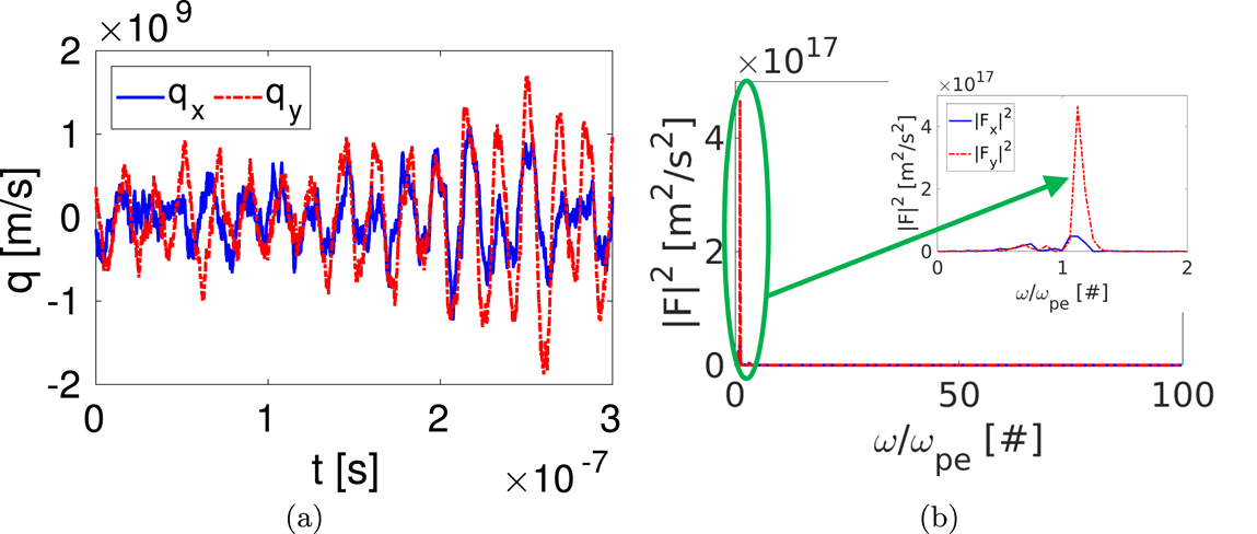
We have simulated a plasma initially at rest, in the absence of an external magnetic or electric field. The results of the frequency analysis are reported in figure 4. The evolution of the quantities
 $q_{x}$
and
 $q_{y}$
(see (3.4)) at time
 $t$
has been depicted in figure 4(a). Instead, in figure 4(b),
 $F_{x}$
and
 $F_{y}$
(namely the FT of respectively
 $q_{x}$
and
 $q_{y}$
) are reported as a function of the frequency
 $\unicode[STIX]{x1D714}$
. The global simulation time
 $T$
is 20 times a plasma oscillation period, so the frequency resolution is
 $\unicode[STIX]{x0394}\unicode[STIX]{x1D714}=2\unicode[STIX]{x03C0}/T=0.05\unicode[STIX]{x1D714}_{pe}$
. The FT (see figure 4
b) shows that the main contribution to the spectrum is given by a single frequency close to the plasma frequency; nonetheless the results along the
 $x$
direction are worse with respect to the
 $y$
axis. In addition, a satisfactory good agreement can be found comparing the value of the frequency for which FT is maximum (respectively
 $\unicode[STIX]{x1D714}_{x}^{\text{SIM}}$
and
 $\unicode[STIX]{x1D714}_{y}^{\text{SIM}}$
) against the expected value
 $\unicode[STIX]{x1D714}_{pe}$
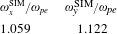
(error of the order of 10 % as reported in table 2). In conclusion, the mild difference between the simulated frequencies and the theoretical one, along with the non-negligible noise in
 $F_{x}$
, are mainly due to the finite simulation domain. In fact, the theoretical derivation of
 $\unicode[STIX]{x1D714}_{pe}$
assumes that we are working with a plasma that is infinite in extent (Chen Reference Chen1984), while we have limited our analysis to a relatively small box (
 $L=2~\text{cm}$
) (Melzani et al.
Reference Melzani, Winisdoerffer, Walder, Folini, Favre, Krastanov and Messmer2013). Therefore, we can conclude that both the field propagation, and particle motion are satisfactorily well described by the EDI code.
In the absence of a magnetic field: (a)
 $q_{x}$
and
 $q_{y}$
(see (3.4)) versus the simulation time
 $t$
; (b) square moduli of the
 $F_{x}$
and
 $F_{y}$
quantities (see (3.3)), namely the FT of
 $q_{x}$
and
 $q_{y}$
, as a function of the frequency
 $\unicode[STIX]{x1D714}$
(normalized in respect to the plasma frequency
 $\unicode[STIX]{x1D714}_{p}$
).

Frequency analysis in the absence of a background magnetic field. Ratio between the plasma frequency (
 $\unicode[STIX]{x1D714}_{pe}$
) and the principal oscillation frequencies calculated from the FT of the
 $q_{x}$
and
 $q_{y}$
quantities (see (3.4)), respectively
 $\unicode[STIX]{x1D714}_{x}^{\text{SIM}}$
and
 $\unicode[STIX]{x1D714}_{y}^{\text{SIM}}$
.

3.2.2 Presence of a background magnetic field
In presence of a uniform magnetic field perpendicular to the simulation domain, particles oscillate with a frequency equal to
 $\unicode[STIX]{x1D714}_{h}$
. However, if the magnetic field is high enough such that
 $\unicode[STIX]{x1D714}_{c}\gg \unicode[STIX]{x1D714}_{pe}$
then
 $\unicode[STIX]{x1D714}_{h}\sim \unicode[STIX]{x1D714}_{c}$
. In our case, assuming
 $B_{0}=1.0~\text{T}$
is enough. Working in these conditions, we have performed the same analysis as that in § 3.2.1 computing the frequency modes of the system. In figure 5(a) the quantities
 $q_{x}$
and
 $q_{y}$
(see (3.4)) are depicted as a function of the time
 $t$
. In figure 5(b) the FTs of both
 $q_{x}$
and
 $q_{y}$
(namely
 $F_{x}$
and
 $F_{y}$
) are reported as a function of the frequency
 $\unicode[STIX]{x1D714}$
. The spectral resolution of this analysis is
 $\unicode[STIX]{x0394}\unicode[STIX]{x1D714}=0.001\unicode[STIX]{x1D714}_{c}$
. In this case the agreement between numerical and theoretical data is very good: the spectrum (see figure 5
b) is peaked, along both
 $x$
and
 $y$
directions, at a frequency very close to the expected
 $\unicode[STIX]{x1D714}_{c}$
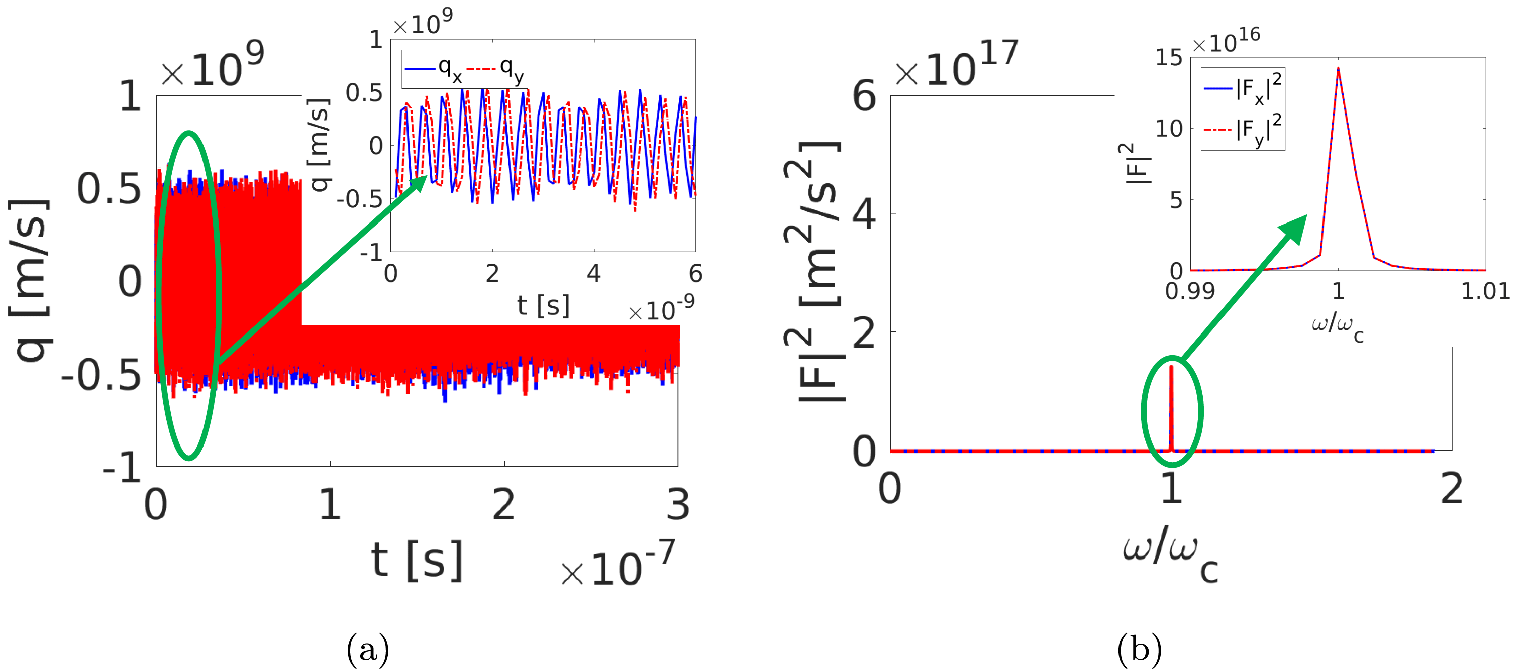
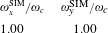
(see table 3). This is a confirmation of the capability of the code in reproducing the particle motion.
In the presence of magnetic field: (a)
 $q_{x}$
and
 $q_{y}$
(see (3.4)) versus the simulation time
 $t$
; (b) square moduli of the
 $F_{x}$
and
 $F_{y}$
quantities (see (3.3)) namely the FT of
 $q_{x}$
and
 $q_{y}$
, as a function of the frequency
 $\unicode[STIX]{x1D714}$
(normalized in respect to the cyclotron frequency
 $\unicode[STIX]{x1D714}_{c}$
).

Frequency analysis in the presence of a background magnetic field. Ratio between the cyclotron frequency (
 $\unicode[STIX]{x1D714}_{c}$
) and the principal oscillation frequencies calculated from the FT of the
 $q_{x}$
and
 $q_{y}$
quantities (see (3.4)), respectively
 $\unicode[STIX]{x1D714}_{x}^{\text{SIM}}$
and
 $\unicode[STIX]{x1D714}_{y}^{\text{SIM}}$
.

3.3 Two stream instability test
In this section we explore the EDI results for the generation of electrostatic waves driven by two stream instability. These waves typically arise from the interaction between two symmetric counterstreaming particle beams, an energetic particle stream injected into a plasma or by setting a current along the plasma where different species can have different drift velocities. These phenomena are discussed in Chen (Reference Chen1984), Birdsall & Langdon (Reference Birdsall and Langdon2004) and Ghorbanalilu, Abdollahzadeh & Rahbari (Reference Ghorbanalilu, Abdollahzadeh and Rahbari2014). A review on this subject is given in Anderson, Fedele & Lisak (Reference Anderson, Fedele and Lisak2001).
3.3.1 Two stream instability formation
We have considered two counterstreaming electron beams with a constant background of ions. The system is initially described by an electron distribution function as reported in (2.21). The first stream travels in the
 $x$
direction with a drift velocity
 $\boldsymbol{v}_{\boldsymbol{D}}=v_{D}\hat{\boldsymbol{x}}$
while the second one moves in the opposite direction with drift velocity
 $\boldsymbol{v}_{\boldsymbol{D}}=-v_{D}\hat{\boldsymbol{x}}$
. If we assume
 $v_{th}\rightarrow 0$
for the loading electrons, i.e.
 $\unicode[STIX]{x1D70E}\rightarrow 0$
(see § 2.6), then each particle has exactly the stream velocity. If we look at periodic harmonic solutions for electric and magnetic fields with pulsation
 $\unicode[STIX]{x1D714}$
and wavevector
 $\boldsymbol{k}$
(e.g.
 $\boldsymbol{E}(\boldsymbol{r},t)=\boldsymbol{E}\text{e}^{\text{i}\boldsymbol{k}\boldsymbol{\cdot }\boldsymbol{r}-\text{i}\unicode[STIX]{x1D714}t}$
), the dispersion relation for longitudinal plasma waves propagating in the
 $x$
direction (
 $\boldsymbol{k}=k\hat{\boldsymbol{x}}$
) in an electron gas described by the Vlasov equation is (Lindman Reference Lindman1970; Bittencourt Reference Bittencourt2013)
 $$\begin{eqnarray}1=\frac{\unicode[STIX]{x1D714}_{pe}^{2}}{k^{2}}\int _{v}\frac{f_{0}(v)}{\left(v_{x}-{\displaystyle \frac{\unicode[STIX]{x1D714}}{k}}\right)^{2}}\,\text{d}v^{2},\end{eqnarray}$$
where
 $f_{0}(v)$
is the electron equilibrium distribution function. Assuming a distribution
 $f_{0}(v)$
equal to the one reported in (2.21), and substituting (2.21) in (3.5) yields
 $$\begin{eqnarray}1=\frac{1}{2}\unicode[STIX]{x1D714}_{pe}^{2}\left[\frac{1}{(kv_{D}-w)^{2}}+\frac{1}{(kv_{D}+w)^{2}}\right].\end{eqnarray}$$
This is the dispersion relation for longitudinal waves in a counterstreaming electron plasma characterized by the distribution reported in (2.21). This equation can be rearranged as a quartic polynomial in
 $\unicode[STIX]{x1D714}$
(Bittencourt Reference Bittencourt2013) with two solutions called
 $\unicode[STIX]{x1D714}_{1}^{2}$
and
 $\unicode[STIX]{x1D714}_{2}^{2}$
. One of these two solutions (say
 $\unicode[STIX]{x1D714}_{2}^{2}$
) is a negative real quantity if
 $$\begin{eqnarray}k^{2}v_{D}^{2}<\unicode[STIX]{x1D714}_{pe}^{2}.\end{eqnarray}$$
It follows that
 $\unicode[STIX]{x1D714}_{2}$
has two imaginary values
 $$\begin{eqnarray}\unicode[STIX]{x1D714}_{2}=\pm \text{i}\unicode[STIX]{x1D714}_{2\text{i}},\end{eqnarray}$$
where
 $\unicode[STIX]{x1D714}_{2\text{i}}$
is a real positive quantity. The positive imaginary value of
 $\unicode[STIX]{x1D714}_{2}$
corresponds to an unstable mode and leads to a growth of instability, while a negative imaginary term in
 $\unicode[STIX]{x1D714}_{2}$
leads to temporal decay of the wave amplitude (Landau damping). Solving (3.6), the positive imaginary value is (Bittencourt Reference Bittencourt2013)
 $$\begin{eqnarray}\unicode[STIX]{x1D714}_{2\text{i}}=\left\{-\left({\textstyle \frac{1}{2}}\unicode[STIX]{x1D714}_{pe}^{2}+k^{2}v_{D}^{2}\right)+\left[\left({\textstyle \frac{1}{2}}\unicode[STIX]{x1D714}_{pe}^{2}+k^{2}v_{D}^{2}\right)^{2}-k^{2}v_{D}^{2}(k^{2}v_{D}^{2}-\unicode[STIX]{x1D714}_{pe}^{2})\right]^{1/2}\right\}^{1/2}\end{eqnarray}$$
and it will be called the growth rate of the instability.
3.3.2 Growth rate, energy and momentum
To test EDI, we have computed the simulated growth rate
 $\unicode[STIX]{x1D714}_{2\text{i}}$
(see Lotov et al.
Reference Lotov, Timofeev, Mesyats, Snytnikov and Vshivkov2015) and compared it with the theoretical growth rate obtained using (3.9). The procedure adopted for calculating
 $\unicode[STIX]{x1D714}_{2\text{i}}$
is described in the following. The energy associated with the electrostatic field
 $W_{E}$
, at a fixed time
 $t$
, can be computed as
 $$\begin{eqnarray}W_{E}=\int _{V}\frac{1}{2}\unicode[STIX]{x1D716}_{0}|\boldsymbol{E}(t)|^{2}\,\text{d}V,\end{eqnarray}$$
where
 $\boldsymbol{E}$
is the electrostatic field,
 $\unicode[STIX]{x1D700}_{0}$
is the vacuum permittivity and the integration is performed on the simulation volume. Equation (3.10) can be discretized as follows
 $$\begin{eqnarray}W_{E}=\frac{1}{2}\unicode[STIX]{x1D700}_{0}\mathop{\sum }_{j}|\boldsymbol{E}_{j}|^{2}\unicode[STIX]{x0394}V_{j},\end{eqnarray}$$
where
 $\boldsymbol{E}_{j}$
is the electric field computed at node
 $j$
,
 $\unicode[STIX]{x0394}V_{j}$
is the covolume associated with node
 $j$
and the sum is made over the number of nodes that define a discretization of the domain. If we consider periodic harmonic solutions for electric field and we assume (3.8) for the unstable mode, it is possible to apply natural logarithm to (3.11) and rewrite it as
 $$\begin{eqnarray}\text{ln}\left(W_{E}\right)=2\unicode[STIX]{x1D714}_{2\text{i}}t+h,\end{eqnarray}$$
where
 $h$
is a constant that is not time dependent. The growth rate can then be estimated as follows
 $$\begin{eqnarray}\unicode[STIX]{x1D714}_{2\text{i}}=\frac{1}{2}\frac{\unicode[STIX]{x2202}}{\unicode[STIX]{x2202}t}\text{ln}(W_{E}).\end{eqnarray}$$
Another important quantity to monitor is the total energy
 $W$
associated with the system. In fact PIC simulations can be affected by numerical heating (Markidis & Lapenta Reference Markidis and Lapenta2011), namely a non-physical growth of
 $W$
. Usually this phenomenon can be reduced by a proper selection of mesh size and integration time step. We can consider the initial energy of the system as its kinetic energy
 $W_{K0}$
, namely the sum of the kinetic energy of ions and electrons
 $W_{K0}\equiv W_{K}^{\text{elec}}+W_{K}^{\text{ion}}$
. In this specific case,
 $W_{K0}\equiv W_{K}^{\text{elec}}$
having assumed fixed ions. Therefore
 $$\begin{eqnarray}W_{K0}=\frac{1}{2}\mathop{\sum }_{i=1}^{N_{sp}}pm_{e}v_{i0}^{2},\end{eqnarray}$$
where
 $N_{sp}$
is the number of electron super-particles in the system,
 $v_{i0}$
is the speed of each super-particle at the initial time step,
 $p$
is the number of particles associated with each super-particle and
 $m_{e}$
is the electron mass. Consequently, the normalized kinetic energy at each time
 $t$
can be computed as suggested by Hu (Reference Hu2016)
 $$\begin{eqnarray}\overline{W}_{K}=\frac{{\displaystyle \frac{1}{2}}\displaystyle \mathop{\sum }_{i=1}^{N_{sp}}pm_{e}v_{i}^{2}}{{\displaystyle \frac{1}{2}}\displaystyle \mathop{\sum }_{i=1}^{N_{sp}}pm_{e}v_{i0}^{2}},\end{eqnarray}$$
where
 $v_{i}$
is the speed of each super-particle at time
 $t$
. Moreover, it is also possible to define the normalized field energy of the system at the time
 $t$
as
 $$\begin{eqnarray}\overline{W}_{E}=\frac{{\displaystyle \frac{1}{2}}\unicode[STIX]{x1D716}_{0}\displaystyle \mathop{\sum }_{j}|\boldsymbol{E}_{j}|^{2}\unicode[STIX]{x0394}V_{j}}{{\displaystyle \frac{1}{2}}\displaystyle \mathop{\sum }_{i=1}^{N_{sp}}pm_{e}v_{i0}^{2}}.\end{eqnarray}$$
Therefore the normalized total energy, in the absence of a magnetic field, can be defined as
 $$\begin{eqnarray}\overline{W}=\overline{W}_{K}+\overline{W}_{E}.\end{eqnarray}$$
Finally, we have monitored the total momentum of the collection of particles
 $\boldsymbol{Q}$
. In fact, due to the charge deposition algorithm that we have adopted (see § 2.4), particles might induce spurious forces on themselves unless the mesh is not rectangularly structured (Colella & Norgaard Reference Colella and Norgaard2010). Therefore the conservation of total momentum might fail due to this effect. At each time
 $t$
, the two components of
 $\boldsymbol{Q}$
, respectively
 $Q_{x}$
along the
 $x$
axis and
 $Q_{y}$
along
 $y$
, are defined as
 $$\begin{eqnarray}\displaystyle & \displaystyle Q_{x}=\mathop{\sum }_{i=1}^{N_{sp}}pm_{e}v_{ix} & \displaystyle\end{eqnarray}$$
 $$\begin{eqnarray}\displaystyle & \displaystyle Q_{y}=\mathop{\sum }_{i=1}^{N_{sp}}pm_{e}v_{iy}, & \displaystyle\end{eqnarray}$$
where
 $v_{ix}$
and
 $v_{iy}$
are the components, along the
 $x$
and
 $y$
axes, of the velocity of the super-particle
 $i$
. Therefore, in order to quantify the effect of self-induced forces, a normalized total momentum has been defined as
 $$\begin{eqnarray}\overline{\boldsymbol{Q}}=\frac{\boldsymbol{Q}}{Q_{0}},\end{eqnarray}$$
where
 $Q_{0}$
is a reference momentum
 $Q_{0}=N_{sp}pm_{e}v_{D}$
, and
 $v_{D}$
is the drift velocity. It is worth recalling that the reference momentum has not been evaluated as the initial total momentum is
 $\boldsymbol{Q}\approx 0$
for
 $t=0$
, provided that the loading distribution function has been assumed in accordance with (2.21).
3.3.3 Numerical analysis
As previously stated, the initial conditions of our simulation consist of two opposite electron beams with drift velocity
 $v_{D}$
and a constant background of ions. More precisely, the initial distribution function
 $f_{0}$
is chosen in accordance with (2.21), where the drift velocity is
 $v_{D}=1\times 10^{6}~\text{m}~\text{s}^{-1}$
. The simulation domain is a square aligned along the
 $x$
and
 $y$
directions, with edge
 $L=2~\text{cm}$
. The dynamics of
 $5\times 10^{5}$
super-particles has been followed; each super-particle is associated with 100 particles. Periodic boundary conditions, namely an electrostatic potential
 $\unicode[STIX]{x1D719}=0$
on the sides of the square, have been adopted. During the simulation, the initial configuration is perturbed with a wave whose wavenumber is
 $k=2\unicode[STIX]{x03C0}/L$
so that, thanks to the periodic boundary conditions, only one unstable mode is selected out of the continuous spectrum typical of the infinite plasma (Ghorbanalilu et al.
Reference Ghorbanalilu, Abdollahzadeh and Rahbari2014).
A convergence study of the numerical accuracy of EDI has been performed as the grid refinement and the integration time step are varied. The numerical accuracy has been evaluated in terms of the difference between the normalized total energy
 $\overline{W}$
at the beginning of the simulation and that when the two stream instability is fully developed (i.e.
 $4\times 10^{-8}~\text{s}$
). In fact, if the grid size and time step are too coarse, PIC simulations can be affected by numerical heating (Markidis & Lapenta Reference Markidis and Lapenta2011). For this application, we have assumed that the total energy cannot vary of more than 2 % because of the latter effect. The simulations have been performed on a machine equipped with an Intel R Core i7-6700HQ CPU 2.60 GHz
 $\times$
8, and 16 Gb of RAM. First the grid refinement effect has been analysed by adopting three different mesh configurations, namely mean edges of the triangular mesh equal to
 $a=8\times 10^{-4}~\text{m}$
(i.e. 2714 triangular elements),
 $a=4\times 10^{-4}~\text{m}$
(10 491 elements) and
 $a=2\times 10^{-4}~\text{m}$
(41 498 elements). In particular, these mesh configurations lead to a simulation parameter
 $n_{a}$
ranging from 3700 up to 14 800, and
 $n_{\unicode[STIX]{x1D706}}$
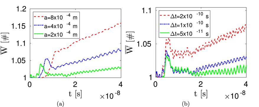
from 1.5 up to 5.0 (see § 2.2). In figure 6(a), the variation of the normalized total energy
 $\overline{W}$
as a function of the time
 $t$
is reported for the three meshes analysed and an integration time step
 $\unicode[STIX]{x0394}t=1\times 10^{-10}~\text{s}$
. Reducing
 $a$
leads to a reduction of the numerical heating (i.e. reduction of the non-physical linear growth of
 $\overline{W}$
for
 $t\geqslant 2\times 10^{-8}~\text{s}$
) as expected (Markidis & Lapenta Reference Markidis and Lapenta2011). Nonetheless, also with the finer mesh size the 2 % threshold is not respected. Therefore, the influence of the integration time step has been investigated, by varying
 $\unicode[STIX]{x0394}t$
from
 $5\times 10^{-11}~\text{s}$
up to
 $2\times 10^{-10}~\text{s}$
(maintaining
 $a=2\times 10^{-4}~\text{m}$
). In particular, the simulation parameter
 $n_{t}$
varies from 45 up to 190 (see § 2.2). From figure 6(b), it can be noticed that the numerical heating decreases with the integration time step. In particular the combination of
 $a=2\times 10^{-4}~\text{m}$
and
 $\unicode[STIX]{x0394}t=5\times 10^{-11}~\text{s}$
leads to a maximum heating lower than 2 %, as required.
Normalized total energy
 $\overline{W}$
(see (3.17)) plotted versus time
 $t$
for: (a) different mean edge of the triangular mesh
 $a$
and fixed integration time step
 $\unicode[STIX]{x0394}t=1\times 10^{-10}~\text{s}$
; (b) different
 $\unicode[STIX]{x0394}t$
and fixed
 $a=2\times 10^{-4}~\text{m}$
.

Timing analysis for different values of the mean edge of the triangular mesh
 $a$
and fixed integration time step
 $\unicode[STIX]{x0394}t=1\times 10^{-11}~\text{s}$
. Reported is the simulation duration, along with the percentage time required for accomplishing the charge deposition (CD), the solution of the electrostatic field (EM), the integration of the particle trajectories (Int) and the particles tracking (Track).

Timing analysis for different values of the integration time step
 $\unicode[STIX]{x0394}t$
and fixed mean edge of the triangular mesh
 $a=2\times 10^{-4}~\text{m}$
. Reported is the simulation duration, along with the percentage time required for accomplishing the charge deposition (CD), the solution of the electrostatic field (EM), the integration of the particle trajectories (Int) and the particles tracking (Track).

For the sake of completeness, the timing analysis for each simulation performed for the convergence study has been reported in tables 4 and 5. Specifically, the simulation duration has been monitored, along with the percentage time required for accomplishing the charge deposition (CD), the solution of the electrostatic field (EM), the integration of the particle trajectories (Int) and the particles tracking (Track); see § 2 for further details on the nomenclature. The simulation duration increases roughly with the square of
 $a$
as does the time required for EM (see table 4). In particular, the computational time for CD, Int and Track are less than quadratic with
 $a$
; therefore the percentage effort required for EM becomes predominant as
 $a$
increases. Moreover, the simulation duration is inversely proportional to
 $\unicode[STIX]{x0394}t$
as the time required for Track (see table 5). Being the computational time for CD, EM and Int almost independent of
 $\unicode[STIX]{x0394}t$
, the percentage effort required for Track decreases with
 $\unicode[STIX]{x0394}t$
.
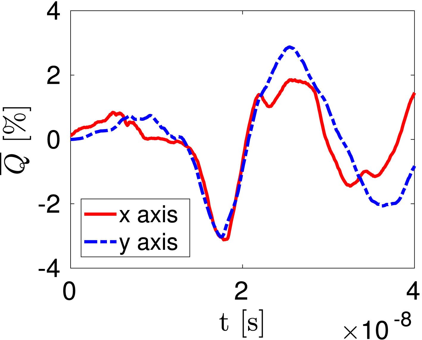
Normalized total momentum
 $\overline{\boldsymbol{Q}}$
(see (3.20)) plotted versus time
 $t$
for mean edge of the triangular mesh
 $a=2\times 10^{-4}~\text{m}$
and integration time step
 $\unicode[STIX]{x0394}t=1\times 10^{-10}~\text{s}$
. Both components along the
 $x$
(solid line) and
 $y$
(dashed line) axes have been depicted.

Finally, we have monitored the normalized total momentum
 $\overline{\boldsymbol{Q}}$
in order to evaluate the effects of the self-induced forces arising because of the adoption of an unstructured and non-uniform grid (Colella & Norgaard Reference Colella and Norgaard2010). The components along the
 $x$
and
 $y$
axes of
 $\overline{\boldsymbol{Q}}$
have been depicted in figure 7 for
 $a=2\times 10^{-4}~\text{m}$
and
 $\unicode[STIX]{x0394}t=5\times 10^{-11}~\text{s}$
. The normalized total momentum presents mild oscillations (amplitude lower than 3 %) whose mean value is approximately zero. Therefore, the self-induced forces do not cause a significant departure from the theoretical condition
 $\overline{\boldsymbol{Q}}=\mathbf{0}$
associated with the absence of external forces acting on the system. Moreover,
 $\overline{\boldsymbol{Q}}$
presents the same features (i.e. mild oscillations around zero) also for the other values of
 $a$
and
 $\unicode[STIX]{x0394}t$
investigated in the convergence analysis. In conclusion, the presence of self-induced forces does not significantly affect the results of the simulation in this application.
3.3.4 Comparison against theoretical results
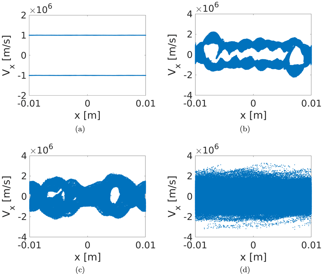
Particle phase space, position along the
 $x$
axis versus component of the velocity in the same direction
 $V_{x}$
. Different times
 $t$
recorded: (a)
 $t=0~\text{s}$
; (b)
 $t=5\times 10^{-9}~\text{s}$
; (c)
 $t=1\times 10^{-8}~\text{s}$
; (d)
 $t=4\times 10^{-8}~\text{s}$
.

In the following, the results obtained with a mesh characterized by
 $a=2\times 10^{-4}~\text{m}$
and an integration time step
 $\unicode[STIX]{x0394}t=5\times 10^{-11}~\text{s}$
, are reported and discussed. In figure 8 the phase space has been reported at different simulation times
 $t$
in order to show the instability formation. In figure 8(a) (
 $t=0~\text{s}$
) it is possible to appreciate the two delta functions that correspond to the initial loading of the particles. Starting from figure 8(b) (
 $t=5\times 10^{-9}~\text{s}$
) it is possible to see the appearance of an electron holes structure. In figure 8(c) (
 $t=1\times 10^{-8}~\text{s}$
) the instability is fully formed. The trapped electrons oscillate inside holes and, as a first approximation, they are governed by the energy conservation (Che Reference Che2016). The adiabatic motions of trapped electrons quickly exchange energy between the electrons and waves (Sagdeev & Galeev Reference Sagdeev and Galeev1969; Che et al.
Reference Che, Drake, Swisdak and Goldstein2013). This leads to the decay of the electric fields and the trapped electrons with higher energy break the confinement of electron holes and escape. The non-adiabatic de-trapping of electrons is irreversible (Sagdeev & Galeev Reference Sagdeev and Galeev1969). Eventually, these coherent structures are destroyed and transform the cold beam into a long hot tail and the plasma becomes warm. This phenomena is shown in figure 8(d) (
 $t=4\times 10^{-8}~\text{s}$
).
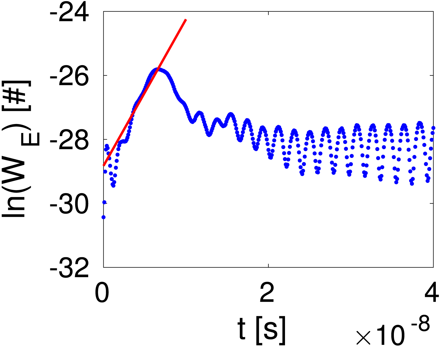
Linear growth rate analysis. Logarithm of the field energy
 $\ln (W_{E})$
versus the simulation time
 $t$
. The red line is the linear fit defined by (3.12) to verify the linear growth rate.

During the growth phase of the instability (figure 8
a,b), most of the kinetic energy
 $W_{K}$
of the beams is converted into the growth of the field energy
 $W_{E}$
. Following the approach proposed in § 3.3.2, we have computed the simulated growth rate and we have compared it with the expected one obtained using (3.9). The results are shown in figure 9 where the red line is the linear fit performed using (3.12). The ratio between the theoretical (
 $\unicode[STIX]{x1D714}_{2\text{i}}^{\text{THEO}}$
) and the simulated (
 $\unicode[STIX]{x1D714}_{2\text{i}}^{\text{SIM}}$
) values of the growth rate is
 $$\begin{eqnarray}\frac{\unicode[STIX]{x1D714}_{2\text{i}}^{\text{THEO}}}{\unicode[STIX]{x1D714}_{2\text{i}}^{\text{SIM}}}=1.021\pm 0.001.\end{eqnarray}$$
The ratio is close to one as expected and the linear dependence, as shown by the fit, is well tested.


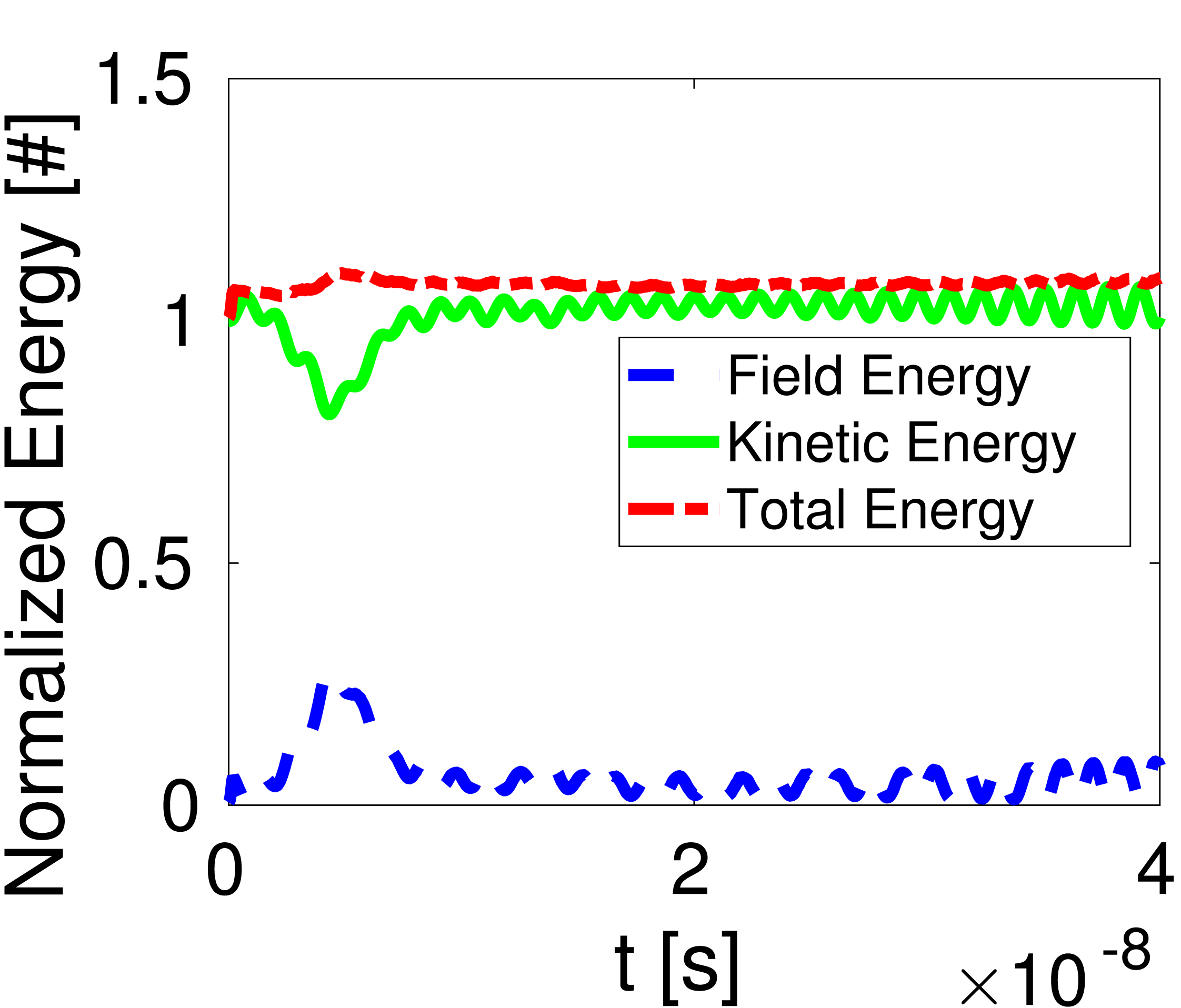
Moreover, the evolution of the energy of the system has been monitored during the entire simulation. Figure 10 displays the normalized total energy
 $\overline{W}$
, kinetic energy
 $\overline{W}_{K}$
and field energy
 $\overline{W}_{E}$
as a function of the simulation time
 $t$
. In particular, it is possible to appreciate that the electrostatic field energy is zero initially, as expected. Between
 $t=0~\text{s}$
and
 $t=5\times 10^{-9}~\text{s}$
there is a conversion of kinetic energy into field energy. The field energy grows with a growth rate
 $\unicode[STIX]{x1D714}_{2\text{i}}$
defined by (3.9), and the linear trend predicted by (3.12) is fully respected. After a time of roughly
 $1/\unicode[STIX]{x1D714}_{2\text{i}}$
from the beginning of the growth rate, the instability starts to thermalize. This leads to a decay of the electric field and, as a consequence, the trapped electrons with higher energy break the confinement of electron holes and escape.
4 Conclusions
In this paper, we have introduced a new electrostatic-magnetostatic PIC code named EDI. The latter is written in C, as it allows for a strong extensibility and reusability in adding, in the future, new models or modify the existing ones. EDI relies on an unstructured mesh of triangles, allowing for arbitrary geometries. Its structure has been explained in detail with particular attention paid to the typical characteristics of PIC codes. If compared with other PIC codes, EDI incorporates an external widely used and versatile solver called GetDP that has been properly modified in order to accept EDI input parameters. This allows us to follow the statement of flexibility, extensibility and efficiency (Verboncoeur et al. Reference Verboncoeur, Langdon and Gladd1995) that should be the basis of every PIC code. EDI has been validated using as test benchmark some classic problems of plasma physics, namely the oscillation modes of a cold plasma, and the two stream instability. Moreover, the correct integration of GetDP on EDI has been checked comparing the results of our solver against FEMM.
Finally, it is worth recalling that further work is needed to make EDI a suitable instrument for the design and the analysis of real systems such as a helicon plasma thruster. First, the full set of Maxwell’s equations needs to be solved in order to properly describe the propagation of the EM waves which characterize the helicon regime (Chen Reference Chen1991). Second, the feeding network needed to provide the power to the thruster must be modelled properly in order to predict the total efficiency of the system. Third, EDI treats currently only 2-D geometries and the dynamics of helicon thrusters presents 2-D axisymmetric characteristics. Nonetheless, a 2-D electrostatic PIC simulation can be employed, for example, to preliminarily estimate the shape of the plasma density and electrostatic potential profiles in the presence of a diverging magnetostatic field (Rao & Singh Reference Rao and Singh2012).
Acknowledgements
We would like to thank Dr D. Rondini, and Professor F. Marzari whose comments helped to improve the quality of this work.