





1 Introduction
The mechanics of flexible filaments on the microscale underpin much of biology, from the propulsive flagella of motile bacteria and spermatozoa to nodal cilia, the latter hypothesised to be responsible for the breaking of left–right symmetry in mammals (Gray Reference Gray1928; Berg & Anderson Reference Berg and Anderson1973; Smith, Montenegro-Johnson & Lopes Reference Smith, Montenegro-Johnson and Lopes2019). Furthermore, the dynamics of elastic filaments is of intense interest in the physics of microdevices and surface flows, including near-wall dynamics. For instance, the consideration of soft deformable sensors has already motivated extensive studies of attached filaments (Roper et al. Reference Roper, Dreyfus, Baudry, Fermigier, Bibette and Stone2006; Guglielmini et al. Reference Guglielmini, Kushwaha, Shaqfeh and Stone2012), as has the characterisation of attached filament forces for understanding the drag induced by slender appendages (Pozrikidis Reference Pozrikidis2011; Curtis et al. Reference Curtis, Kirkman-Brown, Connolly and Gaffney2012; Simons et al. Reference Simons, Olson, Cortez and Fauci2014). Such appendages range from the primary cilium to carbon nanotube mats, with an extensive review of the field presented by du Roure et al. (Reference du Roure, Lindner, Nazockdast and Shelley2019), which notes that both theoretical and numerical developments are very much still required in this field. Indeed, with advances in microscopy enabling ever more detailed quantification of kinematics, often with confining geometry such as a cover slip or substrate, the development of validated, and ideally simple, methodologies would be beneficial in estimating mechanics from kinematics.
Furthermore, the complex mechanics of fluid–structure interaction is an important problem and has been well studied, as illustrated by the slender body theory of Tornberg & Shelley (Reference Tornberg and Shelley2004) and Liu et al. (Reference Liu, Chakrabarti, Saintillan, Lindner and du Roure2018). Numerical simulations that attempt to move past slender body theory are frequently plagued by extensive numerical stiffness, such as the regularised Stokeslet simulations of Olson, Lim & Cortez (Reference Olson, Lim and Cortez2013) and Ishimoto & Gaffney (Reference Ishimoto and Gaffney2018). The recent advance of Moreau, Giraldi & Gadêlha (Reference Moreau, Giraldi and Gadêlha2018) and its subsequent extension by Hall-McNair et al. (Reference Hall-McNair, Gallagher, Montenegro-Johnson, Gadêlha and Smith2019) have sought to address this stiffness, with their methodologies significantly reducing the computational cost associated with filament–fluid interactions via the use of integrated force and moment balance equations, but have not considered even the simplest confined geometry that is an infinite planar wall. Hence our first objective will be to generalise these improved frameworks to dynamics in a half-space bounded by a wall, adapting the recent regularised Stokeslet segment approach of Cortez (Reference Cortez2018) for drag calculations and elastohydrodynamics.
We will validate in detail the computation of drag from kinematic data against the earlier work of Ramia, Tullock & Phan-Thien (Reference Ramia, Tullock and Phan-Thien1993), additionally validating our proposed elastohydrodynamic framework against the gold-standard boundary element method of Pozrikidis (Reference Pozrikidis2010). These validations demonstrate the high accuracy of our approach in capturing the mechanics of filaments, and thus it is of extensive use for understanding cellular swimming. For instance, resistive force theories are very popular due to their ease of use (Lauga et al. Reference Lauga, DiLuzio, Whitesides and Stone2006; Gadêlha et al. Reference Gadêlha, Gaffney, Smith and Kirkman-Brown2010; Sznitman et al. Reference Sznitman, Shen, Sznitman and Arratia2010; Schulman et al. Reference Schulman, Backholm, Ryu and Dalnoki-Veress2014; Utada et al. Reference Utada, Bennett, Fong, Gibiansky, Yildiz, Golestanian and Wong2014; Moreau et al. Reference Moreau, Giraldi and Gadêlha2018), and they have been shown to be of reasonable accuracy in free space for small-bodied cells such as spermatozoa (Johnson & Brokaw Reference Johnson and Brokaw1979). With freedom to choose the resistive coefficients, such local drag theories have been shown to perform very well even near a boundary (Friedrich et al. Reference Friedrich, Riedel-Kruse, Howard and Julicher2010), as supported by the boundary element method validation studies for straight rods of Ramia et al. (Reference Ramia, Tullock and Phan-Thien1993). This suggests that the refinements of Brenner (Reference Brenner1962) and Katz, Blake & Paveri-Fontana (Reference Katz, Blake and Paveri-Fontana1975) to free-space resistive force theories, valid for straight filament motion parallel or perpendicular to a planar wall, may be useful for the analysis of microscopy data, and would be very popular if demonstrated to be accurate. In particular, in the common circumstance where subject cells are imaged swimming parallel to a coverslip, for example Riedel-Kruse & Hilfinger (Reference Riedel-Kruse and Hilfinger2007) and Friedrich et al. (Reference Friedrich, Riedel-Kruse, Howard and Julicher2010), and thus have unchanging boundary separation, we hypothesise that these refined resistive force theories may be sufficient to accurately capture the hydrodynamic drag on a curved filament. Hence, as our second objective and first application, we use the regularised Stokeslet segment framework of Cortez (Reference Cortez2018) to test this hypothesis in exemplar problems. In particular we will consider both the case when a filament is moving parallel to a boundary and the case when it is attached to the surface and moving extensively perpendicular to the wall. Further, the presented elastohydrodynamic framework is sufficiently flexible to enable sophisticated considerations of fluid–structure interactions, inherited from the approach of Moreau et al. (Reference Moreau, Giraldi and Gadêlha2018). Hence, as an application of non-local elastohydrodynamics in a half-space, our final objective is to proceed to demonstrate the methodology’s ease of use in the context of such complex physics by examining the mechanics of a flexible inextensible adhered filament in an oscillatory flow, generalising Pozrikidis’ study of carbon nanomat surface drag to time dependent flows (Pozrikidis Reference Pozrikidis2011).
More generally, testing the boundary-corrected resistive force theories when applied to videomicroscopy data has not been considered in detail. Such evaluation is important for ascertaining whether these corrected resistive force theories may be reliably and accurately used to provide simple access to the viscous drag on filaments in the presence of boundaries, pertinent to the analysis of diverse videomicroscopy data, for example Ohmuro & Ishijima (Reference Ohmuro and Ishijima2006) and Smith et al. (Reference Smith, Gaffney, Blake and Kirkman-Brown2009). Furthermore, the methodology presented is both impactful and a non-trivial extension of previous studies in that it will enable the efficient numerical study of the elastohydrodynamical problem of filament motion near a boundary, once more facilitating the mechanical investigation of a wealth of flagellated microswimmers such as the well-studied human spermatozoon (Fauci & McDonald Reference Fauci and McDonald1995; Elgeti, Kaupp & Gompper Reference Elgeti, Kaupp and Gompper2010; Ishimoto & Gaffney Reference Ishimoto and Gaffney2015). These elastohydrodynamic methods also provide clear precursors for the application of the framework to simulations of oscillating systems in physiological and soft matter modelling, such as primary and motile ciliary systems respectively in the kidneys and lungs, in addition to numerical studies of active surfaces, for example Shum et al. (Reference Shum, Tripathi, Yeomans and Balazs2013) and Balazs et al. (Reference Balazs, Bhattacharya, Tripathi and Shum2014).
2 Methods
2.1 Piecewise-linear filaments
We consider a planar slender inextensible filament represented by
 $N$
piecewise-linear segments of constant length and described by arclength parameter
 $s\in [0,L]$
, where
 $L$
is the filament length. The segment endpoints are taken to correspond to material points, with their positions being denoted
 $\boldsymbol{x}_{1},\ldots ,\boldsymbol{x}_{N+1}$
and where
 $\boldsymbol{x}_{i}$
and
 $\boldsymbol{x}_{i+1}$
correspond to the
 $i$
th segment. We will refer to
 $\boldsymbol{x}_{1}$
as the base of the filament and correspondingly
 $\boldsymbol{x}_{N+1}$
as the tip, and denote the constant arclength associated with the material point
 $\boldsymbol{x}_{i}$
as
 $s_{i}$
. As the filament is assumed to be planar, valid in the absence of external symmetry-breaking features, without loss of generality we assume that it lies in a plane spanned by orthogonal unit vectors
 $\boldsymbol{e}_{x}$
and
 $\boldsymbol{e}_{y}$
, with
 $\boldsymbol{e}_{z}$
completing the orthonormal right-handed triad
 $\boldsymbol{e}_{x}\boldsymbol{e}_{y}\boldsymbol{e}_{z}$
, and we may write
 $\boldsymbol{x}_{i}=x_{i}\boldsymbol{e}_{x}+y_{i}\boldsymbol{e}_{y}$
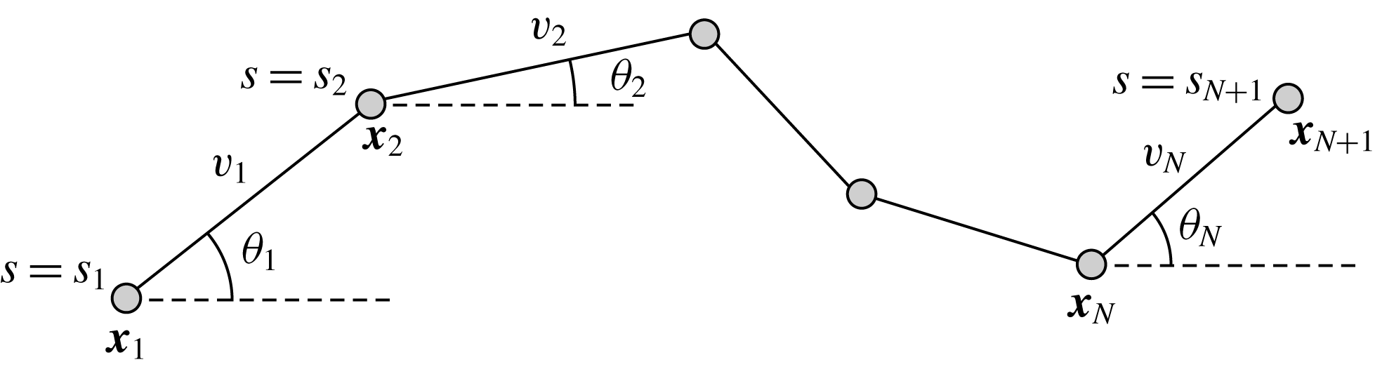
. Following Moreau et al. (Reference Moreau, Giraldi and Gadêlha2018) we note that, once the segment lengths
 $v_{1},\ldots ,v_{N}$
are prescribed, the filament may be completely described by the
 $N+2$
scalars
 $x_{1},y_{1},\unicode[STIX]{x1D703}_{1},\ldots ,\unicode[STIX]{x1D703}_{N}$
, where
 $\unicode[STIX]{x1D703}_{i}$
is defined as the angle between the
 $i$
th segment and the unit vector
 $\boldsymbol{e}_{x}$
as shown in figure 1. Explicitly, from these
 $N+2$
variables we may recover the filament endpoints as
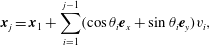 $$\begin{eqnarray}\displaystyle \boldsymbol{x}_{j}=\boldsymbol{x}_{1}+\mathop{\sum }_{i=1}^{j-1}(\cos \unicode[STIX]{x1D703}_{i}\boldsymbol{e}_{x}+\sin \unicode[STIX]{x1D703}_{i}\boldsymbol{e}_{y})v_{i}, & & \displaystyle\end{eqnarray}$$
and, using dots to denote derivatives with respect to time, the velocity of each material point is given by
 $$\begin{eqnarray}\displaystyle \dot{\boldsymbol{x}}_{j}=\dot{\boldsymbol{x}}_{1}+\mathop{\sum }_{i=1}^{j-1}(-\text{sin}\unicode[STIX]{x1D703}_{i}\boldsymbol{e}_{x}+\cos \unicode[STIX]{x1D703}_{i}\boldsymbol{e}_{y})\dot{\unicode[STIX]{x1D703}}_{i}v_{i}, & & \displaystyle\end{eqnarray}$$
again expressible using only the
 $N+2$
variables due to the imposed geometrical constraints.
The two-dimensional piecewise-linear filament. We consider an inextensible filament composed of
 $N$
straight segments each of length
 $v_{i}$
, connected at material points
 $\boldsymbol{x}_{i}$
with each segment making angle
 $\unicode[STIX]{x1D703}_{i}$
with the global
 $\boldsymbol{e}_{x}$
axis. The endpoints
 $\boldsymbol{x}_{1}$
and
 $\boldsymbol{x}_{N+1}$
shall be referred to as the base and tip respectively, and we note that, given segment lengths
 $v_{i}$
, the entire filament may be described by the location of the base and the angles
 $\unicode[STIX]{x1D703}_{i}$
.
2.2 Force distributions via regularised Stokeslet segments
To describe the low Reynolds number fluid dynamics pertinent to the filament we utilise the recent work of Cortez (Reference Cortez2018), namely the method of regularised Stokeslet segments (RSS). Here we briefly recapitulate the formulation of this methodology as presented by Cortez, relating the force density applied on the fluid by the filament to the fluid velocity via non-local hydrodynamics.
As in the popular method of regularised Stokeslets (Cortez Reference Cortez2001), we begin by considering solutions of the three-dimensional smoothly forced Stokes equations, which may be stated for viscosity
 $\unicode[STIX]{x1D707}$
and force
 $\boldsymbol{f}$
applied on the fluid at the origin as
 $$\begin{eqnarray}\displaystyle \unicode[STIX]{x1D707}\unicode[STIX]{x1D6FB}^{2}\boldsymbol{u}=\unicode[STIX]{x1D735}p-\boldsymbol{f}\unicode[STIX]{x1D719}_{\unicode[STIX]{x1D716}},\quad p,\boldsymbol{u}\rightarrow 0\quad \text{as }|\boldsymbol{x}|\rightarrow \infty , & & \displaystyle\end{eqnarray}$$
where
 $\boldsymbol{u}$
is the fluid velocity,
 $p$
is the pressure and
 $\unicode[STIX]{x1D719}_{\unicode[STIX]{x1D716}}$
is a smooth approximation to the Dirac delta distribution dependent on the small parameter
 $\unicode[STIX]{x1D716}$
. Following § 2 of Cortez (Reference Cortez2018) we take
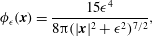 $$\begin{eqnarray}\displaystyle \unicode[STIX]{x1D719}_{\unicode[STIX]{x1D716}}(\boldsymbol{x})=\frac{15\unicode[STIX]{x1D716}^{4}}{8\unicode[STIX]{x03C0}(|\boldsymbol{x}|^{2}+\unicode[STIX]{x1D716}^{2})^{7/2}}, & & \displaystyle\end{eqnarray}$$
for which the solution to (2.3) is known and given by
 $$\begin{eqnarray}\displaystyle 8\unicode[STIX]{x03C0}\unicode[STIX]{x1D707}\boldsymbol{u}(\boldsymbol{x})=\left[\left(\frac{1}{R}+\frac{\unicode[STIX]{x1D716}^{2}}{R^{3}}\right)\unicode[STIX]{x1D644}+\frac{\boldsymbol{x}\boldsymbol{x}^{\top }}{R^{3}}\right]\boldsymbol{f},\quad R(\boldsymbol{x})=\sqrt{|\boldsymbol{x}|^{2}+\unicode[STIX]{x1D716}^{2}}. & & \displaystyle\end{eqnarray}$$
By linearity of the Stokes equations the velocity at a point
 $\tilde{\boldsymbol{x}}$
due to a distribution of regularised Stokeslets along the filament with force density
 $\boldsymbol{f}(s)$
is therefore given by
 $$\begin{eqnarray}\displaystyle 8\unicode[STIX]{x03C0}\unicode[STIX]{x1D707}\boldsymbol{u}(\tilde{\boldsymbol{x}})=\int _{0}^{L}\left[\left(\frac{1}{R(\boldsymbol{r})}+\frac{\unicode[STIX]{x1D716}^{2}}{R(\boldsymbol{r})^{3}}\right)\unicode[STIX]{x1D644}+\frac{\boldsymbol{r}\boldsymbol{r}^{\top }}{R(\boldsymbol{r})^{3}}\right]\boldsymbol{f}(s)\,\text{d}s,\quad \boldsymbol{r}(s)=\tilde{\boldsymbol{x}}-\boldsymbol{x}(s).\quad & & \displaystyle\end{eqnarray}$$
Whilst the original method of regularised Stokeslets would entail approximating the force distribution by a finite number of smoothed point forces, the method of regularised Stokeslet segments instead considers a linear distribution of forces along the straight segments of the discretised filament. With the discretisation of the force distribution as a continuous piecewise-linear function along each of the segments, the fluid velocity is instead given by a sum of integrals over each of the segments, where each individual integral may be analytically evaluated. Parameterising the
 $j$
th segment by
 $\unicode[STIX]{x1D6FC}\in [0,1]$
so that
 $\boldsymbol{x}=\boldsymbol{x}_{j}-\unicode[STIX]{x1D6FC}\boldsymbol{v}$
for
 $\boldsymbol{v}=\boldsymbol{x}_{j}-\boldsymbol{x}_{j+1}$
, and additionally writing the force density as
 $\boldsymbol{f}=\boldsymbol{f}_{j}+\unicode[STIX]{x1D6FC}(\boldsymbol{f}_{j+1}-\boldsymbol{f}_{j})$
for force densities
 $\boldsymbol{f}_{j},\boldsymbol{f}_{j+1}$
at
 $\boldsymbol{x}_{j},\boldsymbol{x}_{j+1}$
respectively, the integral along the
 $j$
th segment is given by
 $$\begin{eqnarray}\displaystyle v_{j}\int _{0}^{1}\left[\left(\frac{1}{R}+\frac{\unicode[STIX]{x1D716}^{2}}{R^{3}}\right)\unicode[STIX]{x1D644}+\frac{(\tilde{\boldsymbol{x}}-\boldsymbol{x}_{j}+\unicode[STIX]{x1D6FC}\boldsymbol{v})(\tilde{\boldsymbol{x}}-\boldsymbol{x}_{j}+\unicode[STIX]{x1D6FC}\boldsymbol{v})^{\top }}{R^{3}}\right][\boldsymbol{f}_{j}+\unicode[STIX]{x1D6FC}(\boldsymbol{f}_{j+1}-\boldsymbol{f}_{j})]\,\text{d}\unicode[STIX]{x1D6FC}, & & \displaystyle\end{eqnarray}$$
where we have identified
 $|\boldsymbol{v}|=v_{j}$
and
 $R=\sqrt{|\tilde{\boldsymbol{x}}-\boldsymbol{ x}_{j}+\unicode[STIX]{x1D6FC}\boldsymbol{ v}|^{2}+\unicode[STIX]{x1D716}^{2}}$
. As noted by Cortez (Reference Cortez2018, § 2.2) this may be written as a sum of integrals of the form
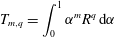 $$\begin{eqnarray}\displaystyle T_{m,q}=\int _{0}^{1}\unicode[STIX]{x1D6FC}^{m}R^{q}\,\text{d}\unicode[STIX]{x1D6FC} & & \displaystyle\end{eqnarray}$$
for
 $(m,q)\in \{(0,-1),(1,-1),(0,-3),(1,-3),(2,-3),(3,-3)\}$
, each of which is implicitly dependent on
 $j$
and may be evaluated by explicit computation of
 $T_{0,-1}$
and
 $T_{0,-3}$
and subsequent application of the recurrence relation
 $$\begin{eqnarray}\displaystyle v_{j}^{2}T_{m+1,q}=-\frac{m}{(q+2)}T_{m-1,q+2}-(\tilde{\boldsymbol{x}}-\boldsymbol{x}_{j})\boldsymbol{\cdot }\boldsymbol{v}T_{m,q}+\frac{1}{q+2}\unicode[STIX]{x1D6FC}^{m}R^{q+2}|_{0}^{1},\quad q\neq -2, & & \displaystyle\end{eqnarray}$$
which follows from the definition of
 $T_{m,q}$
and consideration of
 $(\text{d}/\text{d}\unicode[STIX]{x1D6FC})(\unicode[STIX]{x1D6FC}^{m}R^{q})$
.
The simple extension of this methodology to a half-space bounded by a no-slip planar wall via the image system of Ainley et al. (Reference Ainley, Durkin, Embid, Boindala and Cortez2008) (with the typographical error corrected Smith (Reference Smith2009)) is presented in detail by Cortez (Reference Cortez2018, § 3.3). Exemplified in figure 2, we will consider two configurations of half-space, one in which the infinite planar boundary is parallel to the plane containing the filament, given by
 $z=0$
, and another where the boundary is situated perpendicular to this plane and given by
 $y=0$
. In both cases the hydrodynamics may be described by the same regularised singularity representation, each requiring computation of
 $T_{m,q}$
for the additional values
 $(m,q)\in \{(0,-5),(1,-5),(2,-5),(3,-5),(4,-5),(5,-5)\}$
in order to include the additional necessary regularised singularities. Omitted from the previous work of Cortez, we compute
 $$\begin{eqnarray}\displaystyle T_{0,-5}=\left.\frac{(B+\unicode[STIX]{x1D6FC}C^{2})}{3R^{3}}\frac{(-B^{2}+C^{2}[3A^{2}+4\unicode[STIX]{x1D6FC}B+2\unicode[STIX]{x1D6FC}^{2}C^{2}+3\unicode[STIX]{x1D716}^{2}])}{(B^{2}-C^{2}[A^{2}+\unicode[STIX]{x1D716}^{2}])^{2}}\right|_{0}^{1}, & & \displaystyle\end{eqnarray}$$
where
 $A=|\tilde{\boldsymbol{x}}-\boldsymbol{x}_{j}|$
,
 $B=(\tilde{\boldsymbol{x}}-\boldsymbol{x}_{j})\boldsymbol{\cdot }\boldsymbol{v}$
and
 $C=|\boldsymbol{v}|=v_{j}$
. The remaining values of
 $T_{m,q}$
may be computed via the recurrence relation equation (2.9). Simple computation of the coefficients of the
 $T_{m,q}$
results in a matricial form of the velocity contribution at
 $\tilde{\boldsymbol{x}}$
from the
 $j$
th segment as a linear operator acting on
 $\boldsymbol{f}_{j}$
and
 $\boldsymbol{f}_{j+1}$
, the details of which are cumbersome and given in the supplementary material, available at https://doi.org/10.1017/jfm.2019.723. The overall velocity at the evaluation point
 $\tilde{\boldsymbol{x}}$
is then given by the sum of these contributions, resulting in a matricial equation of the form
 $$\begin{eqnarray}\displaystyle \boldsymbol{u}(\tilde{\boldsymbol{x}})=\unicode[STIX]{x1D648}(\tilde{\boldsymbol{x}})\boldsymbol{F}, & & \displaystyle\end{eqnarray}$$
where
 $\boldsymbol{F}=(f_{1,x},f_{1,y},\ldots ,f_{N+1,x},f_{N+1,y})^{\top }$
herein denotes the composite vector of force densities applied on the fluid at the segment endpoints
 $\boldsymbol{x}_{j}$
in the directions
 $\boldsymbol{e}_{x}$
and
 $\boldsymbol{e}_{y}$
, where we write
 $\boldsymbol{f}_{j}=f_{j,x}\boldsymbol{e}_{x}+f_{j,y}\boldsymbol{e}_{y}$
. Taking the evaluation point
 $\tilde{\boldsymbol{x}}$
as each
 $\boldsymbol{x}_{i}$
in turn yields a square system of linear equations in
 $2(N+1)$
variables, relating the velocities
 $\boldsymbol{u}(\boldsymbol{x}_{i})$
to the force distribution on the filament via non-local hydrodynamics. Application of the no-slip condition at the segment endpoints then gives a relation between the filament velocities and the forces applied on the fluid by the filament, which we write in brief as
 $$\begin{eqnarray}\displaystyle \dot{\boldsymbol{X}}=\unicode[STIX]{x1D63C}\boldsymbol{F}, & & \displaystyle\end{eqnarray}$$
for the square matrix
 $\unicode[STIX]{x1D63C}$
composed row-wise of blocks
 $\unicode[STIX]{x1D648}(\boldsymbol{x}_{i})$
for
 $i=1,\ldots ,N+1$
, and where
 $\dot{\boldsymbol{X}}=({\dot{x}}_{1},{\dot{y}}_{1},\ldots ,{\dot{x}}_{N+1},{\dot{y}}_{N+1})^{\top }$
. Given kinematic data, this linear system may be readily solved to give the force densities applied on the fluid by the filament.
Schematic configurations of planar filaments near boundaries. (a) A filament moving parallel to the infinite planar boundary, at constant separation
 $h$
. The projection of the filament onto the boundary is shown as a thin black line. (b) A filament contained in a plane perpendicular to the boundary, with the plane of motion shown dashed.

2.3 Extension to efficient solution of elastohydrodynamic equations
We now proceed to combine the work of Cortez (Reference Cortez2018) and Moreau et al. (Reference Moreau, Giraldi and Gadêlha2018) to give an efficient scheme for solving non-local planar elastohydrodynamics, similar in concept to the piecewise-constant force density approach of Hall-McNair et al. (Reference Hall-McNair, Gallagher, Montenegro-Johnson, Gadêlha and Smith2019) but with continuous piecewise-linear force discretisation and the additional inclusion of an infinite planar boundary. As formulated by Moreau et al. (Reference Moreau, Giraldi and Gadêlha2018), we integrate the pointwise conditions of force and moment balance on the filament, given by
 $$\begin{eqnarray}\displaystyle & \displaystyle \boldsymbol{n}_{s}-\boldsymbol{f}=\mathbf{0}, & \displaystyle\end{eqnarray}$$
 $$\begin{eqnarray}\displaystyle & \displaystyle \boldsymbol{m}_{s}+\boldsymbol{x}_{s}\times \boldsymbol{n}=\mathbf{0} & \displaystyle\end{eqnarray}$$
for contact force and couple denoted
 $\boldsymbol{n},\boldsymbol{m}$
respectively and where a subscript of
 $s$
denotes differentiation with respect to arclength, noting that we have assumed slenderness of the filament. This yields the integrated equations
 $$\begin{eqnarray}\displaystyle & \displaystyle -\mathop{\sum }_{j=1}^{N}\int _{s_{j}}^{s_{j+1}}\boldsymbol{f}(s)\,\text{d}s=\boldsymbol{n}(0), & \displaystyle\end{eqnarray}$$
 $$\begin{eqnarray}\displaystyle & \displaystyle -\mathop{\sum }_{j=i}^{N}\int _{s_{j}}^{s_{j+1}}(\boldsymbol{x}(s)-\boldsymbol{x}_{i})\times \boldsymbol{f}(s)\,\text{d}s=\boldsymbol{m}(s_{i}),\quad i=1,\ldots ,N. & \displaystyle\end{eqnarray}$$
Here we have assumed conditions of zero contact force and couple at the tip of the filament, i.e.
 $\boldsymbol{n}(L)=\boldsymbol{m}(L)=\mathbf{0}$
, retaining generality at the base for the time being. With the assumption of piecewise-linear distributions of force density
 $\boldsymbol{f}$
over each segment, again with
 $\boldsymbol{f}=\boldsymbol{f}_{j}+\unicode[STIX]{x1D6FC}(\boldsymbol{f}_{j+1}-\boldsymbol{f}_{j})$
on the
 $j$
th segment for
 $\unicode[STIX]{x1D6FC}\in [0,1]$
, we may write these integrals as linear operators on
 $\boldsymbol{F}$
, yielding the system
 $$\begin{eqnarray}\displaystyle -\unicode[STIX]{x1D63D}\boldsymbol{F}=\boldsymbol{R}, & & \displaystyle\end{eqnarray}$$
where
 $\boldsymbol{R}=(\boldsymbol{n}(s_{1})\boldsymbol{\cdot }\boldsymbol{e}_{x},\boldsymbol{n}(s_{1})\boldsymbol{\cdot }\boldsymbol{e}_{y},m(s_{1}),\ldots ,m(s_{N}))^{\top }$
and we are writing
 $\boldsymbol{m}(s_{i})=m(s_{i})\boldsymbol{e}_{z}$
by planarity of the filament. The matrix
 $\unicode[STIX]{x1D63D}$
is of dimension
 $(N+2)\times 2(N+1)$
, which under the assumption of equispaced segment endpoints has rows
 $\boldsymbol{B}_{k}$
given by
 $$\begin{eqnarray}\displaystyle & \displaystyle \boldsymbol{B}_{1}=\frac{\unicode[STIX]{x0394}s}{2}[1,0,2,0,2,\ldots ,2,0,1,0], & \displaystyle\end{eqnarray}$$
 $$\begin{eqnarray}\displaystyle & \displaystyle \boldsymbol{B}_{2}=\frac{\unicode[STIX]{x0394}s}{2}[0,1,0,2,0,2,\ldots ,2,0,1], & \displaystyle\end{eqnarray}$$
with the additional rows
 $\boldsymbol{B}_{i+2}$
each encoding the integrated expression
 $$\begin{eqnarray}\displaystyle \boldsymbol{e}_{z}\boldsymbol{\cdot }\mathop{\sum }_{j=i}^{N}\left\{\left[\frac{\unicode[STIX]{x0394}s}{2}(\boldsymbol{x}_{j}-\boldsymbol{x}_{i})+\frac{\unicode[STIX]{x0394}s^{2}}{6}\boldsymbol{t}_{j}\right]\times \boldsymbol{f}_{j}+\left[\frac{\unicode[STIX]{x0394}s}{2}(\boldsymbol{x}_{j}-\boldsymbol{x}_{i})+\frac{\unicode[STIX]{x0394}s^{2}}{3}\boldsymbol{t}_{j}\right]\times \boldsymbol{f}_{j+1}\right\}, & & \displaystyle\end{eqnarray}$$
where
 $\unicode[STIX]{x0394}s=L/N$
is the length of each segment,
 $\boldsymbol{t}_{j}=\cos \unicode[STIX]{x1D703}_{j}\boldsymbol{e}_{x}+\sin \unicode[STIX]{x1D703}_{j}\boldsymbol{e}_{y}$
is the local unit tangent and
 $i=1,\ldots ,N$
. Thus we may write the coupled elastohydrodynamic problem as
 $$\begin{eqnarray}\displaystyle -\unicode[STIX]{x1D63D}\unicode[STIX]{x1D63C}^{-1}\dot{\boldsymbol{X}}=\boldsymbol{R}, & & \displaystyle\end{eqnarray}$$
where
 $\unicode[STIX]{x1D63D}$
represents integration over segments and
 $\unicode[STIX]{x1D63C}$
encodes the relationship between the forces on the surrounding fluid and the velocities of material points on the filament, here non-local and assumed to be invertible.
As noted in § 2.1, the material velocities
 $\dot{\boldsymbol{x}}_{i}$
may be expressed in terms of the time derivatives of the base point
 $\boldsymbol{x}_{1}$
and the segment angles
 $\unicode[STIX]{x1D703}_{1},\ldots ,\unicode[STIX]{x1D703}_{N}$
. Defining
 $\unicode[STIX]{x1D64C}$
to be the
 $2(N+1)\times (N+2)$
matrix such that
 $$\begin{eqnarray}\displaystyle \unicode[STIX]{x1D64C}\dot{\unicode[STIX]{x1D73D}}=\dot{\boldsymbol{X}}, & & \displaystyle\end{eqnarray}$$
where
 $\unicode[STIX]{x1D73D}=(x_{1},y_{1},\unicode[STIX]{x1D703}_{1},\ldots ,\unicode[STIX]{x1D703}_{N})^{\top }$
, we have
 $\unicode[STIX]{x1D64C}$
given explicitly by

where the subscript
 $P$
denotes that the
 $i$
th row of
 $\unicode[STIX]{x1D64C}$
is to be permuted to
 $$\begin{eqnarray}\displaystyle P(i)=\left\{\begin{array}{@{}ll@{}}2(i-1)+1, & i=1,\ldots ,N+1,\\ 2(i-N-1), & i=N+2,\ldots ,2N+2.\end{array}\right. & & \displaystyle\end{eqnarray}$$
This permutation of
 $\unicode[STIX]{x1D64C}$
allows us to define the blocks
 $\unicode[STIX]{x1D64C}_{1}$
and
 $\unicode[STIX]{x1D64C}_{2}$
as being strictly lower triangular matrices of dimension
 $(N+1)\times N$
with entries
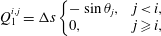 $$\begin{eqnarray}\displaystyle & \displaystyle Q_{1}^{i,j}=\unicode[STIX]{x0394}s\left\{\begin{array}{@{}ll@{}}-\sin \unicode[STIX]{x1D703}_{j}, & j<i,\\ 0, & j\geqslant i,\end{array}\right. & \displaystyle\end{eqnarray}$$
 $$\begin{eqnarray}\displaystyle & \displaystyle Q_{2}^{i,j}=\unicode[STIX]{x0394}s\left\{\begin{array}{@{}ll@{}}+\cos \unicode[STIX]{x1D703}_{j}, & j<i,\\ 0, & j\geqslant i.\end{array}\right. & \displaystyle\end{eqnarray}$$
Given the matrix
 $\unicode[STIX]{x1D64C}$
we may rewrite the full coupled elastohydrodynamic problem simply as
 $$\begin{eqnarray}\displaystyle -\unicode[STIX]{x1D63D}\unicode[STIX]{x1D63C}^{-1}\unicode[STIX]{x1D64C}\dot{\unicode[STIX]{x1D73D}}=\boldsymbol{R}, & & \displaystyle\end{eqnarray}$$
with
 $\unicode[STIX]{x1D63D}\unicode[STIX]{x1D63C}^{-1}\unicode[STIX]{x1D64C}$
being a square matrix of dimension
 $(N+2)\times (N+2)$
. Finally, and here for example assuming force and moment-free conditions at the filament base, the standard linear constitutive relation
 $m(s_{i})=EI\,\unicode[STIX]{x1D703}_{s}(s_{i})\approx EI\,(\unicode[STIX]{x1D703}_{i}-\unicode[STIX]{x1D703}_{i-1})/\unicode[STIX]{x0394}s$
for bending stiffness
 $EI$
, valid for
 $i=2,\ldots ,N$
, gives
 $\boldsymbol{R}$
explicitly in terms of
 $\unicode[STIX]{x1D73D}$
, yielding a linear system of low dimension that may be readily solved for
 $\dot{\unicode[STIX]{x1D73D}}$
, with the temporal dynamics then computable via existing ordinary differential equation (ODE) methods. As noted by Moreau et al., this formulation is readily extensible to the imposition of a variety of boundary conditions, in particular that of a cantilevered filament base, achieved by replacing the overall zero-force and zero-moment equations with
 ${\dot{x}}_{1}={\dot{y}}_{1}=\dot{\unicode[STIX]{x1D703}}_{1}=0$
.
We non-dimensionalise this system by scaling spatial coordinates with filament length
 $L$
, forces with
 $EI/L^{2}$
and time with some characteristic time scale
 $T$
, yielding the non-dimensional system
 $$\begin{eqnarray}\displaystyle -E_{h}\hat{\unicode[STIX]{x1D63D}}\hat{\unicode[STIX]{x1D63C}}^{-1}\hat{\unicode[STIX]{x1D64C}}\dot{\hat{\unicode[STIX]{x1D73D}}}=\hat{\boldsymbol{R}},\quad E_{h}=\frac{8\unicode[STIX]{x03C0}\unicode[STIX]{x1D707}L^{4}}{EI\,T} & & \displaystyle\end{eqnarray}$$
for elastohydrodynamic number
 $E_{h}$
, where the notation
 $\hat{\cdot }$
denotes non-dimensional quantities. The dimensional and non-dimensional quantities are related by
 $$\begin{eqnarray}\displaystyle \unicode[STIX]{x1D63D}=L^{2}\hat{\unicode[STIX]{x1D63D}},\quad \unicode[STIX]{x1D63C}=\frac{1}{8\unicode[STIX]{x03C0}\unicode[STIX]{x1D707}}\hat{\unicode[STIX]{x1D63C}},\quad \unicode[STIX]{x1D64C}\dot{\unicode[STIX]{x1D73D}}=\frac{L}{T}\hat{\unicode[STIX]{x1D64C}}\dot{\hat{\unicode[STIX]{x1D73D}}},\quad \boldsymbol{R}=\frac{EI}{L}\hat{\boldsymbol{R}}, & & \displaystyle\end{eqnarray}$$
where we have multiplied the two force balance equations by
 $\unicode[STIX]{x0394}s=L/N$
and absorbed the dimensional scalings of
 $x_{1},y_{1}$
into
 $\unicode[STIX]{x1D64C}$
for convenience, with
 $\hat{\unicode[STIX]{x1D73D}}=(\hat{x}_{1},{\hat{y}}_{1},\unicode[STIX]{x1D703}_{1},\ldots ,\unicode[STIX]{x1D703}_{N})^{\top }$
. In order to pose the non-dimensional equations in terms of the commonly used sperm number
 $Sp$
(Delmotte, Climent & Plouraboué Reference Delmotte, Climent and Plouraboué2015; Ishimoto & Gaffney Reference Ishimoto and Gaffney2018; Moreau et al.
Reference Moreau, Giraldi and Gadêlha2018), we proceed following Ishimoto & Gaffney (Reference Ishimoto and Gaffney2018) to define
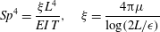 $$\begin{eqnarray}\displaystyle Sp^{4}=\frac{\unicode[STIX]{x1D709}L^{4}}{EI\,T},\quad \unicode[STIX]{x1D709}=\frac{4\unicode[STIX]{x03C0}\unicode[STIX]{x1D707}}{\log (2L/\unicode[STIX]{x1D716})} & & \displaystyle\end{eqnarray}$$
for resistive force coefficient
 $\unicode[STIX]{x1D709}$
and
 $L/\unicode[STIX]{x1D716}=10^{3}$
, giving the approximate relation
 $E_{h}\approx 15.2\,Sp^{4}$
.
2.4 Implementation, verification and parameter choice
Both the calculation of force densities from kinematic data and the solution of full elastohydrodynamics were implemented in MATLAB®. We utilise the inbuilt stiff ODE solver ode15s (Shampine & Reichelt Reference Shampine and Reichelt1997), making use of variable step sizes in order to satisfy configurable error tolerances that are typically set here at
 $10^{-6}$
, with the presented results insensitive to this choice. Prior to the recent work of Hall-McNair et al. (Reference Hall-McNair, Gallagher, Montenegro-Johnson, Gadêlha and Smith2019) the solution of non-local elastohydrodynamics has required significant computational work and minimal timestep for the solution of this stiff problem (Olson et al.
Reference Olson, Lim and Cortez2013; Ishimoto & Gaffney Reference Ishimoto and Gaffney2018), and we replicate in our implementation the low computational cost associated with the integrated elasticity equations of Moreau et al. (Reference Moreau, Giraldi and Gadêlha2018). In particular, typical simulations of a cantilevered filament in background flow, explored in detail in §§ 3.4 and 3.5, have a typical runtime of 10 s, where
 $N=40$
and we simulate over 10 periods of oscillation of the background flow on modest hardware (Intel® Core™ i7-6920HQ CPU).
Verification was first performed on the reduction to an unbounded domain, with the full elastohydrodynamics being verified by comparison with the resistive force theory results of Moreau et al. (Reference Moreau, Giraldi and Gadêlha2018) for filament relaxation. Further drag calculations were compared against the work of Cortez (Reference Cortez2018) for the case of uniform motion, with the degree to which the no-slip condition is numerically satisfied along the filament length having previously been investigated in detail (Cortez Reference Cortez2018, § 3.1). The regularised image system in a half-space was then verified by explicit evaluation of the fluid velocity on the no-slip boundary, with the numerical result being zero to machine precision, and further by noting that far-field results were seen to converge to those of the free-space system. Further qualitative checks were performed, an example being the successful reproduction of the intuitive result that relaxation time scales increase for filaments with reduced separation from the no-slip stationary boundary, along with numerical comparison against the previous works of Pozrikidis regarding the elastohydrodynamics of filaments in steady shear flow (Pozrikidis Reference Pozrikidis2010, Reference Pozrikidis2011), a brief example of which being presented in appendix B. Results of additional verification against the boundary element method of Ramia et al. (Reference Ramia, Tullock and Phan-Thien1993) are shown in figure 3(a). Sufficient accuracy is typically achieved with
 $N=20$
segments, similar to the discretisation used by Cortez (Reference Cortez2018), although we typically take
 $N=40$
to enable the capturing of high-curvature filaments.
As noted by Cortez (Reference Cortez2018), the use of regularised Stokeslet segments allows the regularisation parameter to represent the radius of the filament being modelled, verified here by comparison with the boundary element method of Ramia et al. (Reference Ramia, Tullock and Phan-Thien1993) in figure 3, subject to the phenomenological condition that
 $\unicode[STIX]{x1D716}$
be less than the length of the segments, which appears necessary for convergence. We will take
 $\unicode[STIX]{x1D716}/L=10^{-3}$
unless otherwise stated, with typical slender filament aspect ratios yielding
 $\unicode[STIX]{x1D716}/L$
in the range
 $(10^{-2},10^{-3})$
(Yonekura, Maki-Yonekura & Namba Reference Yonekura, Maki-Yonekura and Namba2003; Ishimoto & Gaffney Reference Ishimoto and Gaffney2016). Whilst the results that follow naturally depend on the size the of the regularisation parameter, it being used as a proxy for the filament radius, this dependence appears to be predominantly quantitative, with the same qualitative conclusions holding across the range of physically relevant values of
 $\unicode[STIX]{x1D716}/L$
.
2.5 Endpoint effects
Inherent to the method of regularised Stokeslet segments as presented here is the presence of apparent large variations in computed force densities at the tips of filaments. This was initially observed by Cortez (Reference Cortez2018, § 3.1, figure 4), who remarked that these endpoint effects may be reduced when
 $\unicode[STIX]{x1D716}/L$
is small. Indeed, for
 $\unicode[STIX]{x1D716}/L$
in our range of physical interest these endpoint effects contribute minimally to overall drag calculations, in particular having little effect on the computed total drag exerted on a filament and the computed force densities away from the filament tip, whose presentation we focus on herein. Exploration of the effects of non-uniform segment lengths yields the observation that these oscillatory endpoint effects remain limited to approximately the 3 segments proximal to the ends of the filament, thus the integral contribution of these oscillations may be reduced by the clustering of segments near the filament tips. For our typical parameters of
 $N=40$
and
 $\unicode[STIX]{x1D716}/L=10^{-3}$
we observe a difference in integrated drag along of filaments of less than 2 % between linear, quadratic and Chebyshev segment endpoints, hence we proceed with calculations utilising segments of uniform length.
2.6 Boundary-corrected resistive force theory
The leading-order approximation of slender body hydrodynamics that is resistive force theory (RFT) was first introduced by Gray and Hancock (Hancock Reference Hancock1953; Gray & Hancock Reference Gray and Hancock1955), relating the local drag on a body to its local tangential and normal velocities
 $u_{t},u_{n}$
via
 $$\begin{eqnarray}\displaystyle f_{t}=-C_{t}u_{t},\quad f_{n}=-C_{n}u_{n}. & & \displaystyle\end{eqnarray}$$
Here
 $f_{t},f_{n}$
are the local tangential and normal components of force applied on the fluid, with the constant resistive coefficients
 $C_{t},C_{n}$
typically being functions of filament aspect ratio. As RFT relates forces only to local velocities, calculations using this simple local drag theory are not able to account for the presence of a boundary. Brenner (Reference Brenner1962) and Katz et al. (Reference Katz, Blake and Paveri-Fontana1975) posed corrections to resistive force theory for straight filaments in asymptotic regimes far from or near to an infinite no-slip boundary, with the latter having been verified against high-accuracy boundary element methods by Ramia et al. (Reference Ramia, Tullock and Phan-Thien1993). In the case of filament motion confined to a plane parallel to the boundary, as exemplified in figure 2(a), by this wall-corrected resistive force theory (W-RFT) a straight filament parallel to the boundary has resistive coefficients given by
 $$\begin{eqnarray}\displaystyle C_{t}=\frac{2\unicode[STIX]{x03C0}\unicode[STIX]{x1D707}}{\log \left({\displaystyle \frac{2}{\unicode[STIX]{x1D716}}}\right)-0.807-{\displaystyle \frac{3L}{8h}}},\quad C_{n}=\frac{4\unicode[STIX]{x03C0}\unicode[STIX]{x1D707}}{\log \left({\displaystyle \frac{2}{\unicode[STIX]{x1D716}}}\right)+0.193-{\displaystyle \frac{3L}{4h}}}\quad \text{if }L\ll h,\quad \qquad & & \displaystyle\end{eqnarray}$$
 $$\begin{eqnarray}\displaystyle C_{t}=\frac{2\unicode[STIX]{x03C0}\unicode[STIX]{x1D707}}{\log \left({\displaystyle \frac{2h}{\unicode[STIX]{x1D716}}}\right)},\quad C_{n}=\frac{4\unicode[STIX]{x03C0}\unicode[STIX]{x1D707}}{\log \left({\displaystyle \frac{2h}{\unicode[STIX]{x1D716}}}\right)}\quad \text{if }L\gg h, & & \displaystyle\end{eqnarray}$$
where
 $h$
is the boundary separation of the filament and
 $\unicode[STIX]{x1D716}$
has been taken as the filament radius. Similarly, and as in figure 2(b), when aligned parallel to the boundary and moving in a plane perpendicular to the surface the coefficients are given by
 $$\begin{eqnarray}\displaystyle C_{t}=\frac{2\unicode[STIX]{x03C0}\unicode[STIX]{x1D707}}{\log \left({\displaystyle \frac{2}{\unicode[STIX]{x1D716}}}\right)-0.807-{\displaystyle \frac{3L}{8h}}},\quad C_{n}=\frac{4\unicode[STIX]{x03C0}\unicode[STIX]{x1D707}}{\log \left({\displaystyle \frac{2}{\unicode[STIX]{x1D716}}}\right)+0.193-{\displaystyle \frac{3L}{2h}}}\quad \text{if }L\ll h,\quad \qquad & & \displaystyle\end{eqnarray}$$
 $$\begin{eqnarray}\displaystyle C_{t}=\frac{2\unicode[STIX]{x03C0}\unicode[STIX]{x1D707}}{\log \left({\displaystyle \frac{2h}{\unicode[STIX]{x1D716}}}\right)},\quad C_{n}=\frac{4\unicode[STIX]{x03C0}\unicode[STIX]{x1D707}}{\log \left({\displaystyle \frac{2h}{\unicode[STIX]{x1D716}}}\right)-1}\quad \text{if }L\gg h, & & \displaystyle\end{eqnarray}$$
where all coefficients are as summarised by Brennen & Winet (Reference Brennen and Winet1977) and (2.35) and (2.33) additionally require
 $\unicode[STIX]{x1D716}\ll h$
. In free space we will adopt the resistive force coefficients defined by the large-
 $h$
limit of (2.32) and (2.34), and refer to this simpler theory as free-space resistive force theory (F-RFT). As given by Brenner and Katz et al., the leading-order boundary corrections to
 $C_{t}$
and
 $C_{n}$
are
 $O(L/h)^{3}$
when
 $L\ll h$
, and
 $O(h/L)$
when
 $L\gg h$
, although the overall error in the resistive force approximation remains logarithmic in the filament aspect ratio.
3 Results and applications
3.1 Evaluation of wall-corrected resistive force theory for straight filaments
For the case of a straight uniform filament aligned parallel to a planar boundary, utilising the approach of § 2.2 we compute the hydrodynamic drag on the slender body as it moves parallel to the wall along its tangent at unit non-dimensional velocity, comparing the solutions given by the methods of regularised Stokeslet segments, free-space RFT and wall-corrected RFT, solving separately (2.12) and (2.31) for force density. Having normalised by the F-RFT solution, it being independent of the boundary separation
 $h$
, we show the computed non-dimensional total drag in figure 3. Good agreement near the boundary can be seen between the W-RFT of Katz et al. and our implementation of the method of regularised Stokeslet segments, the former as previously validated in the limit
 $h/L\rightarrow 0$
with high-accuracy boundary element methods by Ramia et al. (Reference Ramia, Tullock and Phan-Thien1993). Indeed, direct comparison of the RSS solution with Ramia et al. (Reference Ramia, Tullock and Phan-Thien1993, figure 4c) provides additional verification of our methodology, where we note that for this comparison we are taking
 $\unicode[STIX]{x1D716}/L=10^{-2}$
to ensure the filament radius matches that used in the boundary element computations. Further, far from the boundary the correction of Brenner (Reference Brenner1962) lies within 10 % of the RSS solution, evidencing good overall agreement between the two schemes as the normalised wall separation
 $h/L$
increases. Analogous agreement between these methodologies can additionally be seen for total normal drag when moving normal to the boundary, thus we conclude that the corrections to resistive force theory of Brenner and Katz et al. agree closely with regularised Stokeslet segments for straight filaments in their respective asymptotic regimes. Hence, agreement in more generality may be reasonably hypothesised.
Expressions for corrected drag coefficients pertaining to filaments oriented perpendicular to a planar boundary are also available in the literature, and may be found summarised in the work of Brennen & Winet (Reference Brennen and Winet1977). Repetition of the above validation, translating the filament along its axis and again comparing against the gold-standard boundary element method of Ramia et al. (Reference Ramia, Tullock and Phan-Thien1993), yields similar conclusions regarding the validity of near and far-field expressions for the resistive coefficients. The same good far-field agreement can be seen between the RSS solution and the corrected resistive force theory, however the near-boundary corrected theory has no dependence on boundary separation in the limit and thus does not capture near-boundary variations in drag. With significant experimental and theoretical study concerning filaments aligned approximately parallel to a boundary, for example the theoretical works of Elgeti et al. (Reference Elgeti, Kaupp and Gompper2010) and typical videomicroscopy data of Ohmuro & Ishijima (Reference Ohmuro and Ishijima2006) and Smith et al. (Reference Smith, Gaffney, Blake and Kirkman-Brown2009), herein we focus on the expressions given in § 2.6 and on the validity of resistive force theories in more generality.
Computed total drag on a straight parallel filament moving along a boundary parallel to its tangent, here with
 $\unicode[STIX]{x1D716}/L=10^{-2}$
. (a) Near the boundary we see very good agreement between the regularised Stokeslet segment (RSS) solution (dot-dashed) and the wall-corrected resistive force theory (W-RFT) solution of Katz et al. (solid), with the latter corresponding to (2.33) and fair agreement maintained outside the region of validity of W-RFT as
 $h/L\sim 1$
. The boundary element method (BEM) data of Ramia et al. are marked with squares, adapted from Ramia et al. (Reference Ramia, Tullock and Phan-Thien1993, figure 4c) and show good agreement with the regularised Stokeslet segments. (b) Similar agreement can be seen far from the boundary, with the asymptotic solution of Brenner given in (2.32) losing validity when
 $h/L\sim 1$
although remaining within 10 % of the RSS solution.

3.2 Computing hydrodynamic drag on filaments parallel to boundaries
Following the established good agreement of W-RFT and RSS for straight filaments we proceed to evaluate the agreement for curved filaments moving in a plane parallel to the no-slip boundary, again solving (2.12) and (2.31). Motivated by the previous use of free-space resistive force theory for drag determination from captured kinematic data (Friedrich et al.
Reference Friedrich, Riedel-Kruse, Howard and Julicher2010; Gaffney et al.
Reference Gaffney, Gadêlha, Smith, Blake and Kirkman-Brown2011; Ishijima Reference Ishijima2011; Ooi et al.
Reference Ooi, Smith, Gadelha, Gaffney and Kirkman-Brown2014), we compute the forces on a free filament from the kinematic data of Ishimoto et al. (Reference Ishimoto, Gadêlha, Gaffney, Smith and Kirkman-Brown2017) corresponding to the flagellum of a human spermatozoon. These data, captured from free-swimming spermatozoa situated approximately
 $10{-}20~\unicode[STIX]{x03BC}\text{m}$
from a planar boundary, were smoothed by Ishimoto et al. (Reference Ishimoto, Gadêlha, Gaffney, Smith and Kirkman-Brown2017) and given in the form of an arclength parameterisation, with approximately 100 frames being recorded per beat cycle.
Drag calculations from kinematic data captured parallel to a planar boundary, with data from Ishimoto et al. (Reference Ishimoto, Gadêlha, Gaffney, Smith and Kirkman-Brown2017). (a) The tangential and normal components of the drag along the filament for a single frame (upper and lower panels respectively) at separation
 $h/L=0.01$
, showing good qualitative agreement between methodologies of drag computation and fair quantitative agreement between W-RFT and RSS. (b) The magnitude and direction of the total integrated force on the filament (upper and lower panels respectively) at separation
 $h/L=0.01$
, with direction measured relative to an arbitrary fixed axis. As in (a), agreement is fair and qualitative features are captured by all methodologies. Remarkably, the direction of the resultant force as computed using the resistive force theories strongly agrees with that of the non-local RSS. Endpoint effects are visible in the upper panel of (a), as discussed in detail in § 2.5. (c) Ratio of effective drag coefficients
 $C_{n}/C_{t}$
, as computed via RSS, against boundary separation (upper), shown as the median over all frames and all material points (740 frames, 100 points per frame). The ratio as predicted by Katz et al., 2, is shown as a dashed line for comparison. Error bars corresponding to half the interquartile range are shown, representative of dispersal about the median as the distributions do not appear significantly skewed. Modifying the kinematic data of Ishimoto et al. (Reference Ishimoto, Gadêlha, Gaffney, Smith and Kirkman-Brown2017) as described in the main text to simulate a pinned filament, analogous results are shown in red (dotted, thin), highlighting a reduction in validity of resistive force theories for pinned data but retaining notable accuracy when very close to the boundary. The lower panel is a histogram corresponding to
 $h/L=0.01$
, showing the distribution of effective coefficient ratios in the free-swimming case, highlighting tight grouping about the median. (d) Median values of effective resistive coefficients against boundary separation (upper), with error bars of half the interquartile range. Pinned data are shown in red (dotted, thin) for comparison. The lower panel is a histogram corresponding to
 $h/L=0.01$
, showing the tight distribution of dimensionless effective drag coefficients
 $C_{n}/\unicode[STIX]{x1D707}$
and
 $C_{t}/\unicode[STIX]{x1D707}$
, with
 $C_{t}/\unicode[STIX]{x1D707}$
shown darker. Medians are shown dashed.

We first consider the filament moving in very close proximity to the boundary, with normalised separation
 $h/L=0.01$
, within the typical range of slithering motion for spermatozoa (Nosrati et al.
Reference Nosrati, Driouchi, Yip and Sinton2015). A summary of the resulting drag calculations is shown in figure 4, from which we observe that the wall-corrected RFT of Katz et al. (Reference Katz, Blake and Paveri-Fontana1975) can demonstrate strong pointwise agreement with regularised Stokeslet segments over a single frame (figure 4
a). However, calculations of the total drag force over the filament highlight a general trend of over-estimation of force densities by W-RFT, with the differences between W-RFT and RSS having a median of 37 % over the 100 frame range shown here, with differences measured relative to the RSS value. Free-space resistive force theory appears to do the opposite, systematically underestimating the magnitude of total drag, with increased median deviation of 45 % from the RSS solution. Most notable however is the tight clustering of the effective ratio of drag coefficients
 $C_{n}/C_{t}$
, shown in figure 4(c), computed pointwise from the RSS solution and with an analogous distribution of the effective values of
 $C_{n}/\unicode[STIX]{x1D707}$
and
 $C_{t}/\unicode[STIX]{x1D707}$
shown in figure 4(d). This suggests that an appropriate choice of resistive coefficient would enable the accurate approximation of local filament drag using only a local theory, in concurrence with the findings of Friedrich et al. (Reference Friedrich, Riedel-Kruse, Howard and Julicher2010) though seen here much closer to the boundary and at a local level, rather than Friedrich et al.’s comparison to observed sperm behaviour, which necessarily averages over the cell. We verify this result using additional waveform data, modifying the kinematic data of Ishimoto et al. (Reference Ishimoto, Gadêlha, Gaffney, Smith and Kirkman-Brown2017) to crudely approximate a pinned spermatozoa by fixing both the endpoint and local tangent in space, along with the idealised pinned waveforms used by Curtis et al. (Reference Curtis, Kirkman-Brown, Connolly and Gaffney2012) given in appendix C. In particular, the tight clustering of effective coefficient ratios at low boundary separations is retained, though we note reduced agreement compared to that present for free-swimming data. Surprisingly, these coefficients and ratios do not align with the corrected coefficients of Katz et al. (Reference Katz, Blake and Paveri-Fontana1975), derived for straight filaments parallel to a boundary.
Additionally, for approximate separations
 $0.3<h/L<1$
we observe very strong agreement between resistive force theories and the non-local solution, with median differences in total drag between methodologies consistently less than 15 %, in many cases being less than 5 %. This is coupled with additional agreement concerning the direction of the resultant filament drag, which is retained even at reduced separations (figure 4
b, lower). However, lost at such intermediate separations is any clear choice of effective resistive coefficient ratio, with the distribution of effective ratios significantly broadening above
 $h/L\approx 0.05$
.
At a much greater distance from the boundary, with
 $h/L=10$
, as expected F-RFT and W-RFT give approximately equal estimates for the drag on the free-swimming filament, with the W-RFT solution having approached that of F-RFT. As in the case of near-boundary swimming, only small differences are present between the W-RFT and RSS solutions, with median differences between methods of approximately 6 %, in this case with the magnitude of all computed drag forces having been reduced from their near-wall values by approximately a factor of two. Thus, in the medium and far field of a boundary resistive force theories appear remarkably accurate for determining the total drag on even curved filaments moving parallel to the boundary, although surprisingly at this increased boundary separation there is little grouping of the effective resistive coefficient ratios.
3.3 Hyperactivation-induced tugging of tethered spermatozoa
Explored initially by Curtis et al. (Reference Curtis, Kirkman-Brown, Connolly and Gaffney2012) using both free-space and wall-corrected resistive force theory, and reconsidered by Simons et al. (Reference Simons, Olson, Cortez and Fauci2014) using regularised Stokeslets, we re-evaluate the observation that the hyperactivation of mammalian spermatozoa aids in surface escape via a beat-induced tugging effect on the tether point of boundary-attached spermatozoa, and consider in detail the drag on the filament. Adopting the idealised beat patterns used by Curtis et al. and given in appendix C, appropriately non-dimensionalised, we position the base of the filament
 $0.01L$
from the boundary and compute both the total and local drag from this kinematic data for both hyperactivated and normal beating, noting that the plane of filament beating is perpendicular to the boundary. Mirroring the set-up of Curtis et al., we assume that the filament is clamped at its base, implemented by rotating the kinematic data to align the basal tangent in each instant at some angle
 $\unicode[STIX]{x1D703}_{0}$
to the boundary.
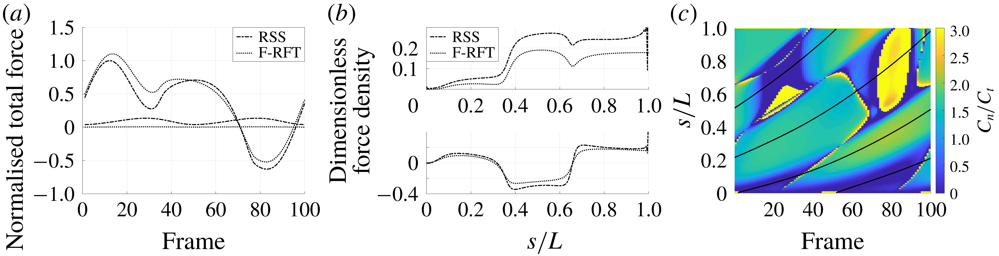
Figure 5 shows the results of the drag computation over a single beat period for both the hyperactivated and normal beat patterns for
 $\unicode[STIX]{x1D703}_{0}=\unicode[STIX]{x03C0}/2$
. We see reaffirmed by the method of regularised Stokeslet segments the conclusion of Curtis et al., with the hyperactivated beat pattern exhibiting a change of sign in force component perpendicular to the boundary, whilst no such change is observed for the normally beating flagellum. Sampling
 $\unicode[STIX]{x1D703}_{0}\in [\unicode[STIX]{x03C0}/4,\unicode[STIX]{x03C0}/2]$
, we note that this observation holds across a range of basal orientations for these beat patterns, in agreement with the RFT-established conclusions of Curtis et al. Overall, figure 5(a) demonstrates fair agreement between the local free-space resistive force theory solution and that obtained using regularised Stokeslet segments, suggesting a surprising validity in using simple local theories in this circumstance, as concluded broadly by Simons et al.. However, the pointwise values of the drag density highlight a stark disagreement between local and non-local theories, with deviations of up to 43 % for the tangential component of the drag for the frame of hyperactivated beating shown in figure 5(b). For reference, the integrated total drag along the filament on average gives differences of only 24 % between RSS and F-RFT, suggesting that a serendipitous cancellation occurs when integrating over the flagellum.
In figure 5(c) we show the ratio of effective tangential and normal drag coefficients for the hyperactivated beating, along with contours of zero curvature for reference. Significant variation in this ratio can be seen, in stark contrast to those computed for near-wall parallel swimming above. Thus the conclusion of Friedrich et al. (Reference Friedrich, Riedel-Kruse, Howard and Julicher2010), that resistive force theory is accurate to high precision, does not hold for a bound spermatozoon, and hence the use of simple resistive force theories for near-boundary drag calculations is not reliable in general. This precludes the general use of the near-boundary correction of Katz et al. (Reference Katz, Blake and Paveri-Fontana1975) in this circumstance, supported by the poor agreement seen in figure 5, whilst the far-field result of Brenner (Reference Brenner1962) is inappropriate in such close boundary proximity.
Drag computation for pinned spermatozoa with a base clamped perpendicular to a boundary over a single period of 100 frames. (a) Normalised total force on the boundary over a single beat period as computed by regularised Stokeslet segments (dot-dashed) and free-space resistive force theory (dotted), in the cases of hyperactive and normal beating patterns (high and low amplitudes respectively). Normal beating gives rise to a force on the boundary of unchanging sign, whilst hyperactivated beating generates a force whose sign changes over the beat period, corresponding to a so-called tugging effect. (b) Tangential (upper panel) and normal components (lower panel) of force density as a function of arclength for a single frame, shown for the hyperactivated beat pattern. In contrast to the fair agreement between methods seen in (a), with mean error of 24 % for the hyperactivated beat between F-RFT and RSS, tangential force density differs on average by 43 % between methods for the frame shown. (c) Ratio between effective drag coefficients computed using regularised Stokeslet segments, with contours of zero filament curvature superimposed as black curves, showing significant variation in the effective ratio.
3.4 Morphological bifurcation of cantilevered filaments in an oscillatory flow
In the absence of a resistive force theory capable of accurately quantifying the details of pinned filament motion perpendicular to boundaries, we extensively utilise the non-local theory of regularised Stokeslet segments to consider the fully coupled elastohydrodynamics of a cantilevered filament in an oscillating background flow, as formulated in § 2.3. With a planar infinite no-slip boundary situated at
 ${\hat{y}}=0$
and the filament base located at
 $(\hat{x},{\hat{y}})=(0,0.01)$
to avoid numerical degeneracy, we consider the non-dimensional background flow with velocity
 $\hat{\boldsymbol{u}}_{b}=\hat{a}\sin (2\unicode[STIX]{x03C0}\hat{t}-\hat{t}_{0}){\hat{y}}\boldsymbol{e}_{x}$
for amplitude
 $\hat{a}$
and phase
 $\hat{t}_{0}$
. Note that this flow preserves symmetry in the plane containing the filament, thus we may retain the assumption of filament planarity. Hence we have the modified non-dimensional system
 $$\begin{eqnarray}\displaystyle -E_{h}\hat{\unicode[STIX]{x1D63D}}\hat{\unicode[STIX]{x1D63C}}^{-1}\hat{\unicode[STIX]{x1D64C}}\dot{\hat{\unicode[STIX]{x1D73D}}}=\hat{\boldsymbol{R}}-E_{h}\hat{\unicode[STIX]{x1D63D}}\hat{\unicode[STIX]{x1D63C}}^{-1}\hat{\boldsymbol{U}}_{b}, & & \displaystyle\end{eqnarray}$$
where the components of
 $\hat{\boldsymbol{U}}_{b}$
are given by the background flow evaluated at the endpoints of filament segments, explicitly
 $$\begin{eqnarray}\displaystyle \hat{\boldsymbol{U}}_{b}=\hat{a}\sin (2\unicode[STIX]{x03C0}\hat{t}-\hat{t}_{0})({\hat{y}}_{1},0,{\hat{y}}_{2},\ldots ,{\hat{y}}_{N+1},0)^{\top }. & & \displaystyle\end{eqnarray}$$
Noting that
 $\boldsymbol{n}(s_{1})$
and
 $\boldsymbol{m}(s_{1})$
are a priori unknown for a cantilevered filament, we impose the appropriate constraints of
 ${\dot{x}}_{1}=\dot{y_{1}}=\dot{\unicode[STIX]{x1D703}}_{1}=0$
in place of the total force and moment-balance equations, again yielding a square linear system. Under the assumption of a straight initial configuration with
 $\unicode[STIX]{x1D703}_{i}=\unicode[STIX]{x03C0}/2$
for
 $i=1,\ldots ,N$
, which we make throughout, there is freedom in the three non-dimensional parameters
 $\hat{a}$
,
 $\hat{t}_{0}$
and
 $E_{h}$
, the latter being equivalent to the sperm number
 $Sp$
. In appendix A we consider in detail the effects on the dynamics of varying the phase
 $\hat{t}_{0}$
of the background flow, concluding that phase can effectively be neglected in long-time dynamics, and thus we will fix
 $\hat{t}_{0}=0$
, noting that this breaks the inherent left–right symmetry of the initial condition.
For fixed
 $\hat{a}$
we consider the beating of the filament as it is driven by the background flow with the sperm number being varied. With
 $\hat{a}=2\unicode[STIX]{x03C0}$
, we showcase in figure 6 the diverse range of observed behaviours. For low sperm numbers, in this case below a threshold value of around
 $Sp=2.5$
, we observe symmetric, low amplitude beating of the filament. Increasing the sperm number beyond this point results in the remarkable emergence of an asymmetric beating, shown in figure 6(b), strongly resembling the characteristic beating of a cilium. In particular, we see reproduced in this passive, flow-driven filament the defining power and recovery strokes of beating cilia (Brennen & Winet Reference Brennen and Winet1977).
Periodic beating of a cantilevered filament in oscillatory background flow of amplitude
 $\hat{a}=2\unicode[STIX]{x03C0}$
, shown here over a single period of the background flow after convergence to periodic filament motion has occurred. (a) At low sperm numbers, here with
 $Sp=1.14$
, flow-driven beating is approximately symmetric. (b) For medium sperm numbers a remarkable ciliary-type asymmetric beating emerges, shown here for
 $Sp=2.84$
and globally stable, with a clear distinction between effective forward and reverse strokes. (c) At higher sperm numbers the filament buckles significantly and regains a symmetric periodic beat, here with
 $Sp=4.55$
. (d–f) Plots of signed curvature corresponding to (a–c) above, sampled at 100 frames per period and each independently scaled for clarity, with select contours of curvature shown. Symmetry is clearly visible in (d) and (f), with the latter displaying a low-order buckling mode. (e) Exemplifies cilia-like beating, with the effective power stroke occurring approximately between frames 20 and 60 (shown black, dashed).
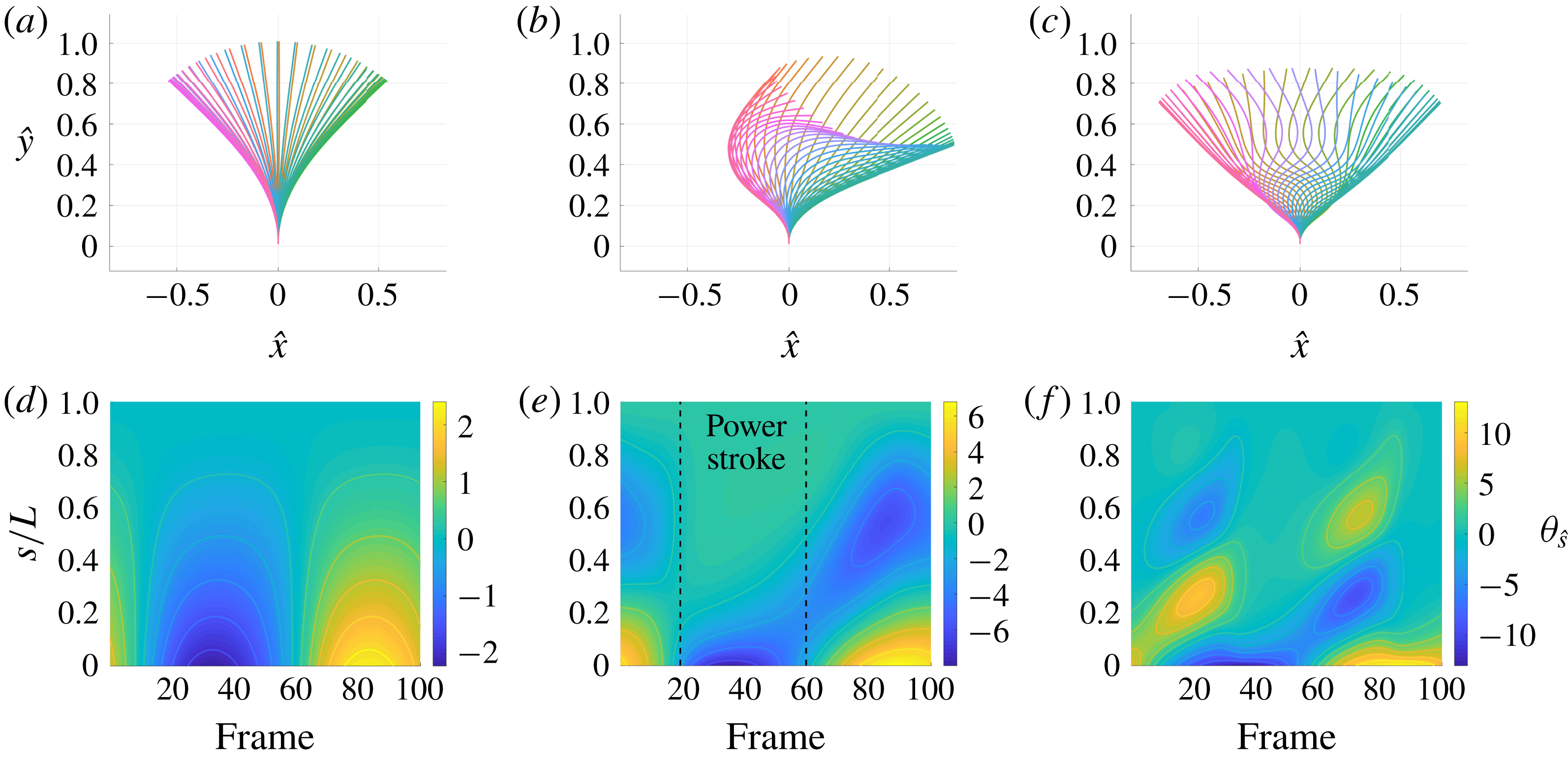
Increasing the sperm number further results in the filament buckling and its beating regaining approximate symmetry, as can be seen in figure 6(c) for
 $Sp=4.55$
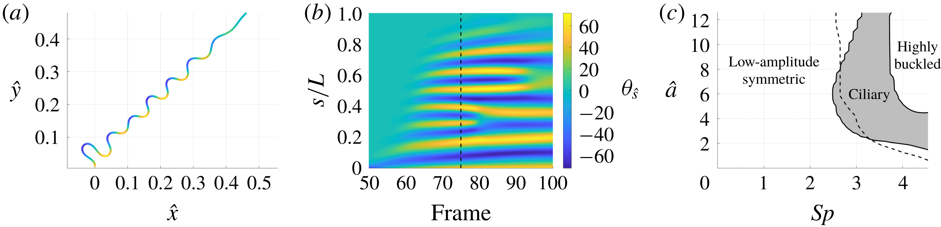
. For very high sperm numbers we see the appearance of buckling modes of higher order, resolved in figure 7 using
 $N=150$
segments to capture filaments with such exceptionally high curvatures. With such high sperm numbers, we observe the collapse of modes onto those corresponding to lower-order buckling as time progresses, in addition to a greatly increased relaxation time to periodic beating in comparison to stiffer filaments.
In order to classify the mode of periodic beating we introduce the symmetry measure
 $S$
, defined for our piecewise-linear filament with segment endpoint coordinates
 $\hat{\boldsymbol{x}}_{i}(\hat{t})$
as
 $$\begin{eqnarray}\displaystyle S=1-\frac{1}{2}\int \frac{\displaystyle \mathop{\sum }_{i}|H\hat{\boldsymbol{x}}_{i}(\hat{t})-\hat{\boldsymbol{x}}_{i}(\hat{t}+1/2)|^{2}}{\displaystyle \mathop{\sum }_{i}|\hat{\boldsymbol{x}}_{i}(\hat{t})|^{2}}\,\text{d}\hat{t}, & & \displaystyle\end{eqnarray}$$
where
 $H\hat{\boldsymbol{x}}_{i}$
denotes the reflection of
 $\hat{\boldsymbol{x}}_{i}$
in the plane
 $\hat{x}=0$
, and the integral over
 $\hat{t}$
runs over half the period of the motion after convergence to periodic beating has occurred. We note that the left–right symmetric beats of figures 6(a) and 6(c) give
 $S=1$
, with motion that breaks left–right symmetry such as the distinct forward and reverse strokes of ciliary beating yielding reduced values of
 $S$
. We find that values of
 $S$
a small tolerance less than unity indeed correspond well to the ciliary-type beating of figure 6(b). We additionally distinguish between approximately straight and highly buckled beating by considering the number of filament regions with curvature of unchanging sign, classifying filaments with three or more such regions as buckled. Shown in figure 7(c) are the regions of the
 $Sp{-}\hat{a}$
parameter space that approximately correspond to low-amplitude symmetric, ciliary and buckled modes of filament beating.
Bifurcation into high-order buckling modes for a filament with high sperm number, here with
 $Sp=16$
and sampled at 100 frames over the initial period of the background flow. (a) A single frame of the initial motion of the filament, where high-curvature regions can be seen to be resolved by the
 $N=150$
segments used here, with curvature represented by colour. (b) The curvature of the filament over the latter part of the initial period of the background flow, from which we may identify the collapse of high-order modes onto lower-order buckling modes. The frame shown in (a) is indicated on the curvature plot by a dashed line, with colour scalings consistent between plots. (c) A bifurcation diagram highlighting the regions of parameter space corresponding to low-amplitude symmetric, ciliary and buckled modes of beating. Buckled modes appear to the right of the dividing dashed line, as defined by the transition between less than three and three regions of constant curvature sign along the filament. Furthermore, ciliary beating occurs within contours delimiting where
 $S$
is essentially unity, shown shaded. In the overlap region between ciliary and buckled beating we observe ciliary-type beats with buckled tips.
3.5 Time-averaged total drag on cantilevered filaments in oscillatory flow corresponds to distinct beating morphologies
Computation of the total hydrodynamic drag exerted on the filament by the background oscillatory flow over a single period reveals a bifurcation structure closely aligned with that of the morphology of beating. Shown in figure 8(a) and rescaled by flow amplitude, the normalised total drag in the direction parallel to the boundary is seen to be of constant sign, and minimal for the approximately symmetric beating present at low sperm numbers, with a region of non-trivial total drag appearing for
 $Sp\approx 1$
where elastic effects further distance the beating from reciprocal motion. Figure 8(c) demonstrates that such minimal total drag arises as the result of gross cancellation over the period of oscillation, consistent with the symmetry of the associated beating mode. Upon entering the region of parameter space consistent with ciliary-type beating there is a significant change in the magnitude of the experienced total drag, intuitively correlated with the emergence of the distinct forward and backward strokes of ciliary beating. With reference to the bifurcation diagram of figure 7(c), highly buckled beating at high values of
 $Sp$
results in little total drag in the direction parallel to the boundary, consistent with the truly time-reversible motion obtained in the limit of (3.1) as
 $E_{h}\rightarrow \infty$
. Notably, the direction of the time-averaged drag exerted on the filament over a period of the background flow points in the direction of the power stroke; with reference to the motion shown in figure 6(b), this corresponds to a resultant drag in the direction of increasing
 $\hat{x}$
, opposite in direction to the resultant drag that might be expected to act on an actively beating cilium in otherwise stationary fluid.
Hydrodynamic drag associated with cantilevered filaments in oscillating flow over a single period. (a) Total drag on the filament in the direction parallel to the boundary, averaged over a single period. A steep increase in total drag is noted to occur upon entering the parameter regime of ciliary beating, with a less-prominent local maximum present around
 $Sp=1$
. (b) Total pushing force applied on the base of the filament in the direction perpendicular to the boundary over a single period of the background flow. A clear maximum can be seen around
 $Sp=1$
, corresponding to the symmetric beating of stiff filaments, with the high sperm number border of the ciliary region being aligned with a sharp, albeit limited increase in total drag for
 $\hat{a}>6$
. (c) Maximum instantaneous total drag on the filament in the direction parallel to the boundary. Comparison with (a) highlights gross total drag cancellation occurring for low
 $Sp$
, with reduced cancellation for the asymmetric ciliary-type beating. (d) Maximum absolute instantaneous force applied on the base of the filament in the direction perpendicular to the boundary. By comparison with (b) we observe limited cancellation of total drag in this direction in stiff filaments, with significant cancellation occurring for ciliary-type beating. Each panel is normalised by the maximum instantaneous total parallel drag and rescaled by flow amplitude to enable meaningful comparison. Select contours of total drag are shown and the region of ciliary-type beating is outlined in black, the latter determined only from the kinematic symmetry measure
 $S$
.
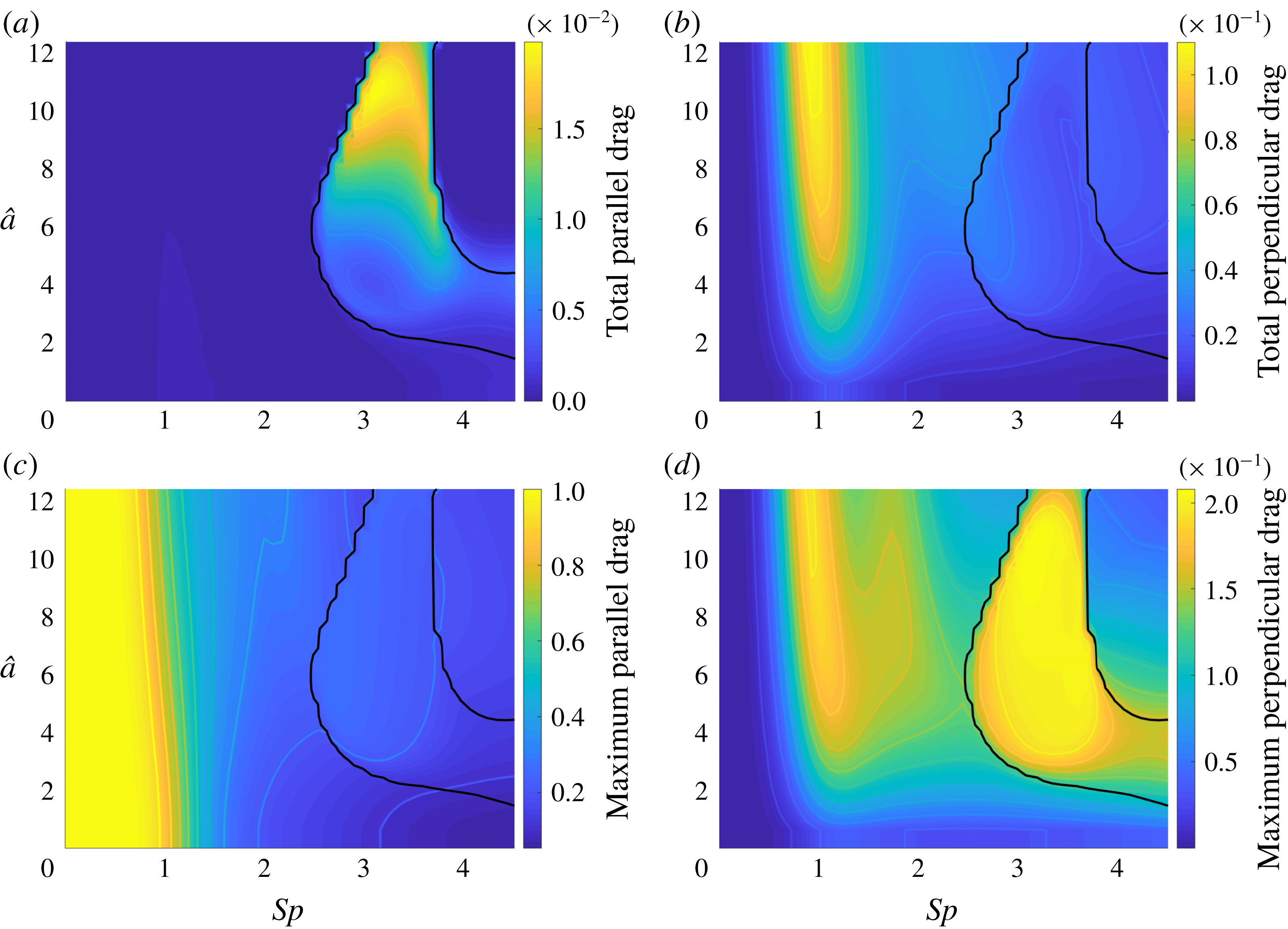
Considering similarly the total force applied on the filament base in the direction normal to the boundary over a single beat period, we again observe that the total force is of constant sign, corresponding to the filament pushing towards the boundary. Shown in figure 8(b), the maximal force occurs around
 $Sp=1$
for the majority of sampled flow amplitudes, aligning with the local maximum of total parallel drag noted previously and pertaining to the non-reciprocal symmetric beating of stiff filaments. Comparison with figure 8(d) reveals in this case that significant total drag cancellation occurs for the asymmetric ciliary-type beating. In contrast, the total drag on stiffer filaments in this direction sees limited cancellation, exemplifying the significance of beating morphology in filament drag calculations.
4 Discussion
In this work we have examined the accuracy of resistive force theories in quantifying the mechanics of planar filament motion in a half space via regularised Stokeslet segments, further exploring the coupled non-local elastohydrodynamics of cantilevered filaments in an oscillatory flow. We have seen that the corrections to free-space resistive force theory of Brenner (Reference Brenner1962) and Katz et al. (Reference Katz, Blake and Paveri-Fontana1975) perform well both in the near and far field of planar boundaries when applied to straight filaments, in agreement with the verification of Ramia et al. (Reference Ramia, Tullock and Phan-Thien1993) and serving as additional validation of our methodology.
By considering the motion of curved filaments in planes parallel to a boundary, in line with our hypothesis we have found that these corrections capture quantitative filament dynamics to moderate accuracy in all but the most extreme boundary proximities. Remarkably however, when very close to the boundary we have nonetheless observed a tightly distributed ratio of effective drag coefficients, and indeed tightly distributed coefficients, suggesting that a resistive force theory with such coefficients could yield accurate estimates for hydrodynamic drag in this circumstance. With subjects imaged in the relative near field of a coverslip, the similar conclusion of Friedrich et al. (Reference Friedrich, Riedel-Kruse, Howard and Julicher2010) is thus in part supported by our non-local calculations, albeit here at greatly reduced boundary separations, and suggests the future development of an accurate, empirical resistive force theory in the near field of boundaries. This has potential application to the study of a slithering mode of swimming, as reported to be prevalent in spermatozoa by Nosrati et al. (Reference Nosrati, Driouchi, Yip and Sinton2015) although this mode is far from ubiquitous. Analytical exploration of this result would require consideration of the asymptotic limit where the separation of singularities from their images is much less than the length scale of the filament radius of curvature, with such detailed calculations expected to be a subject of significant future study.
We have seen that the agreement between methodologies for parallel-swimming filaments does not carry through to those moving in a plane perpendicular to the boundary, with no clear consensus on effective coefficient ratio for pinned filaments moving perpendicular to boundaries. Thus we conclude that constant-coefficient resistive force theories cannot be expected to give accuracy comparable to non-local methods for filaments moving perpendicular to boundaries. Despite this, here we have reverified the conclusion of Curtis et al. (Reference Curtis, Kirkman-Brown, Connolly and Gaffney2012), based originally on resistive force theory, although this appears to rely on serendipitous cancellations on integrating along the filament.
In particular, we have noted a potential lack of reliability in local drag theories when applied to pinned filaments, as evidenced by the loss of coherence in effective drag coefficient ratio when using artificially pinned kinematic data in § 3.2, supported further by the findings of § 3.3 for tethered spermatozoa. Accordingly, we have utilised the non-local hydrodynamics of Cortez (Reference Cortez2018) to examine the response of a cantilevered elastic filament to an oscillatory background flow, with this application highlighting the flexibility in our treatment of the coupled elastohydrodynamics. Having established convergence to a single limiting periodic behaviour from a range of initial conditions for fixed filament and flow parameters, as detailed in appendix A, we have evidenced in passive flow-driven filaments the existence of a remarkable mode of beating typically characteristic of actively beating cilia. Notably, the fact that the movement of our passive filaments appears qualitatively similar to that of actively beating cilia highlights that one cannot naively infer internal mechanics by simply observing filament motion alone.
The asymmetric ciliary-type mode of beating was found to be accompanied by two distinct highly symmetric beating modes. Most prevalent in the
 $Sp{-}\hat{a}$
parameter space was that of low-amplitude beating, with the pinned filament retaining low curvature throughout and generating the maximal time-averaged total normal force into the boundary amongst beating morphologies. Highly buckled modes corresponding to less-rigid filaments produced minimal time-averaged total drag over each period of the background flow, with the high-order buckling modes still resolved by our piecewise-linear formulation of the governing elastohydrodynamics. The near symmetry of each of these modes resulted in little time-averaged total drag in the direction parallel to the boundary. In contrast, entering the region of parameter space corresponding to ciliary beating is seen to strongly correlate with a sharp increase in time-averaged total parallel drag, intuitively the result of kinematic asymmetry arising from the distinct power and recovery strokes of ciliary beating. Hence, elastohydrodynamically induced morphological changes in general have a dramatic effect on filament drag mechanics. Furthermore, the efficiency of the presented methodology would facilitate in-depth mechanical studies of primary cilia with regards to transmitted force and mechanotransduction, noting that the interaction of bending modulus variations, effective boundary conditions at the ciliary base, changes in cross-section of the cilium and cilium length are reported to be under-explored even in the restricted context of renal physiology (Nag & Resnick Reference Nag and Resnick2017). Additionally, the methodology as presented here is readily extensible, with the potential to enable efficient multi-filament elastohydrodynamic simulations applicable to the study of a variety of physical and biological systems, such as actively driven ciliary carpets or carbon nanotube mats. An interesting additional direction, although requiring significant further modelling development, is generalising this framework to non-planar filament motions, as would occur with symmetry-breaking background flows.
In summary, we have considered in detail the validity of traditional and corrected resistive force theories for filaments in the presence of a planar boundary, concluding that, whilst in general these local drag theories may not be relied upon to perform well against non-local solutions for curved filaments, for filament motion parallel to a boundary the use of a resistive force theory may be remarkably accurate with appropriately chosen coefficients, and viable over a range of boundary separations. Verified against previous high-accuracy methods, we have additionally presented an efficient non-local formulation of the governing elastohydrodynamics in a half-space, exemplifying its flexibility by application to a cantilevered filament in oscillatory flow. This study of passive filaments revealed a surprising asymmetric beating morphology found typically in active cilia, highlighting a complex relationship between passive elastic fibres, internally forced filaments, the flows that they drive and the forces that they induce.
Acknowledgements
B.J.W. is supported by the UK Engineering and Physical Sciences Research Council (EPSRC), grant EP/N509711/1. K.I. is supported by JSPS-KAKENHI for Young Researchers (18K13456), JSPS Overseas Research Fellowship (29-0146) and MEXT Leading Initiative for Excellent Young Researchers (LEADER).
The research materials supporting this publication can be accessed at http://dx.doi.org/10.5287/bodleian:MzdNe99JY.
Supplementary material
Supplementary material is available at https://doi.org/10.1017/jfm.2019.723.
Appendix A. Influence of flow phase on cantilevered filament dynamics
One might expect the phase
 $\hat{t}_{0}$
of the background oscillatory flow of § 3.4 to have significant impact on long-time filament dynamics, the most notable of such effects being the selection of left–right polarity in resulting behaviours. We examine the long-time dynamics for a range of phases, flow amplitudes and elastohydrodynamic numbers, tracking in particular the maximally attained displacement of the filament tip from the centreline
 $\hat{x}=0$
throughout each period of the background flow, denoted
 $\hat{x}_{max}$
and exemplified by figure 9(a). In particular, convergence of
 $\hat{x}_{max}$
to a constant would serve to validate, a posteriori, the assumption of periodic motion. Sampling
 $Sp$
and
 $\hat{a}$
each from the range
 $[0.5,12]$
, as expected we observe a duality in solutions inherited from the left–right symmetry of the problem, and we additionally note the convergence of all solutions to a single periodic motion, where the period is aligned with that of the background flow to working precision. This is demonstrated by figure 9(b), which shows the evolution of
 $\hat{x}_{max}$
over a number of cycles of the background flow for
 $Sp=3.13$
and
 $\hat{a}=2\unicode[STIX]{x03C0}$
. We see convergence of all solutions to a common limit cycle of periodic behaviour, with even the approximately symmetric transient motion of
 $\hat{t}_{0}=\unicode[STIX]{x03C0}/2$
(shown dashed) eventually collapsing onto the same mode of behaviour. Hence we resolve that exploration of the
 $Sp$
–
 $\hat{a}$
parameter space, holding
 $\hat{t}_{0}$
constant, is sufficient to capture the long-time behaviours of the cantilevered filament system.
Evaluating the sensitivity of long-time behaviour to background flow phase. (a) An illustration of the measure
 $\hat{x}_{max}$
used to determine periodicity and convergence of filament behaviour, equal to the maximal displacement of the filament tip from the centreline over one period of the background flow. Filament configurations throughout one period of motion are shown as coloured curves. (b) The evolution of
 $\hat{x}_{max}$
over 40 periods of the background flow, for various choices of initial phase
 $\hat{t}_{0}\in [0,\unicode[STIX]{x03C0}]$
, here for
 $Sp=3.13$
,
 $\hat{a}=2\unicode[STIX]{x03C0}$
. In the upper panel we see that all choices of
 $\hat{t}_{0}$
lead to convergence to the same behaviour, with even the approximate initial symmetry of the
 $\hat{t}_{0}=\unicode[STIX]{x03C0}/2$
instance (dashed) collapsing onto the common limiting behaviour. A posteriori validation of convergence to periodic motion from all phases is provided by consideration of the per cycle change in
 $\hat{x}_{max}$
, as shown in the lower panel and highlighting eventual periodicity. Symmetric counterparts for
 $\hat{t}_{0}\in [\unicode[STIX]{x03C0},2\unicode[STIX]{x03C0}]$
have been omitted. (c) Signed curvature of the filament during the first periods of the background flow, with select contours of curvature shown, and sampled at 100 frames per period for
 $\hat{t}_{0}=3\unicode[STIX]{x03C0}/8$
, showing the transition to ciliary beating from a straight initial configuration.
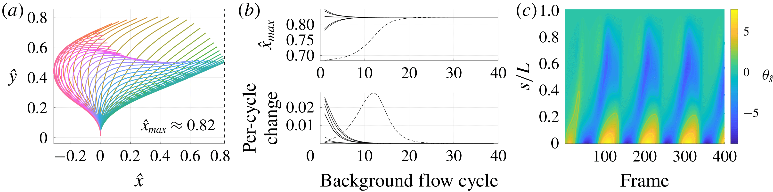
Appendix B. Validation of elastohydrodynamics in a half-space
Here we present an example verifying our implementation of our methodology for simulating filament elastohydrodynamics in a half-space via comparison to the boundary element computations of Pozrikidis, with data adapted from Pozrikidis (Reference Pozrikidis2010, figure 11). Given a stationary background shear flow of unit dimensionless shearing rate, so that
 $\hat{\boldsymbol{u}}_{b}={\hat{y}}\boldsymbol{e}_{x}$
in the notation of § 3.4, we simulate the motion of a passive cantilevered filament attached to a planar boundary until convergence of the filament to a stationary solution. Taking
 $E_{h}\approx 34,68,85$
in turn, in figure 10 we show the resulting filament shapes against those found in the work of Pozrikidis (Reference Pozrikidis2010). The remarkable agreement between the boundary element computations of Pozrikidis and our solution for the filament shape serves as a further validation of our methodology, and in particular demonstrates the capability of our proposed scheme to accommodate non-trivial background flows and filament boundary conditions.
The limiting deflections of cantilevered filaments in background shear flows, with elastohydrodynamic numbers
 $E_{h}\approx 34,68,85$
(black, solid), compared with data adapted from Pozrikidis (Reference Pozrikidis2010, figure 11) and corresponding to
 $\hat{E}_{B}=1.0,0.5,0.4$
from the publication of Pozrikidis. The latter data are shown as red circles, with good agreement between solutions, serving as validation of our treatment and implementation of the governing elastohydrodynamics. Here
 $N=80$
and
 $\unicode[STIX]{x1D716}/L=0.05$
, the latter in line with the set-up of Pozrikidis (Reference Pozrikidis2010).
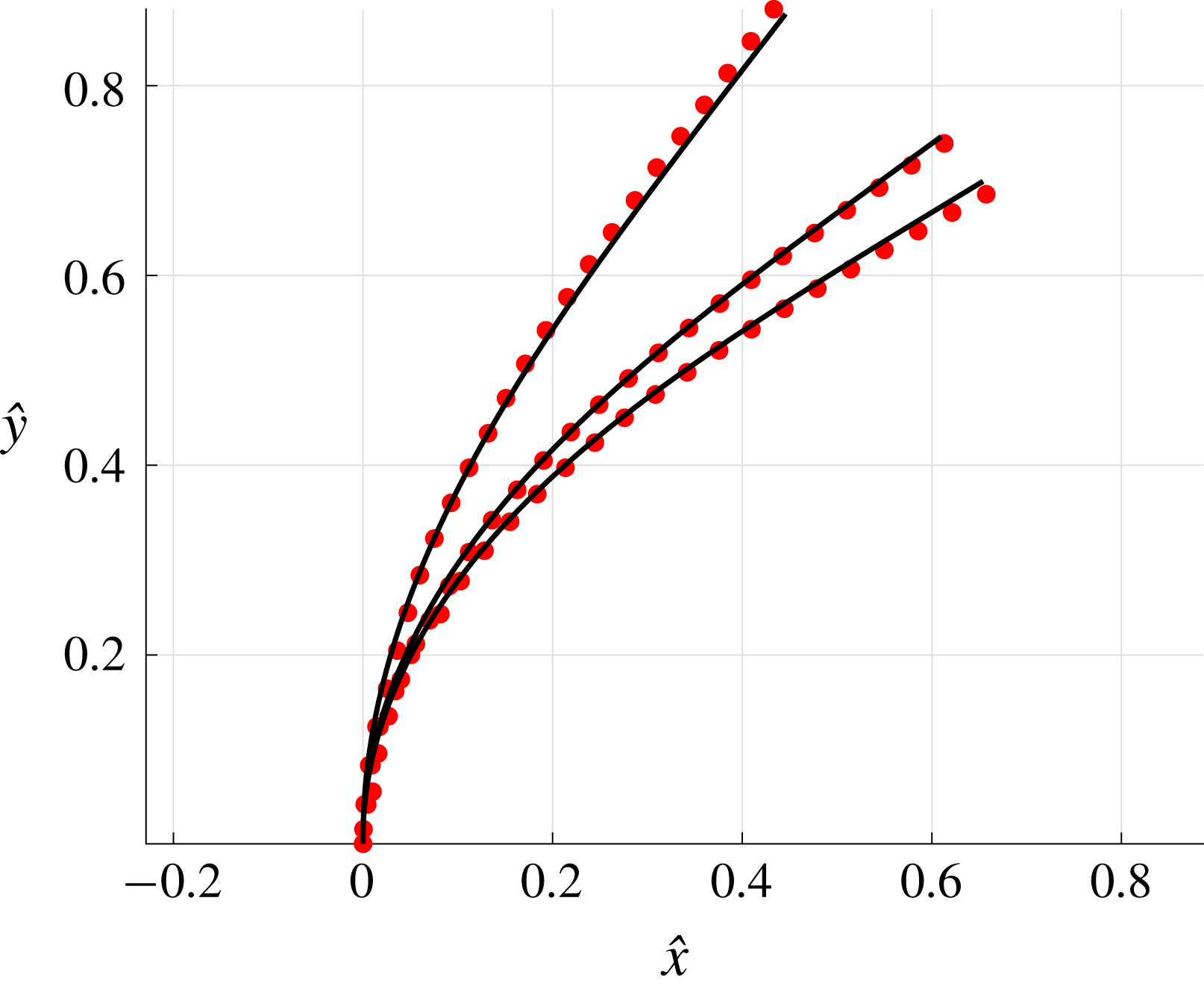
Appendix C. Kinematic data used in Curtis et al.
With
 $\hat{x},{\hat{y}}$
here denoting dimensionless coordinates, the flagellar waveforms of Curtis et al. (Reference Curtis, Kirkman-Brown, Connolly and Gaffney2012) used in §§ 3.2 and 3.3 may be parameterised as
 $$\begin{eqnarray}\displaystyle & \displaystyle \hat{x}(\unicode[STIX]{x1D709},\hat{t})=\unicode[STIX]{x1D709}, & \displaystyle\end{eqnarray}$$
 $$\begin{eqnarray}\displaystyle & \displaystyle {\hat{y}}(\unicode[STIX]{x1D709},\hat{t})=A_{N}\unicode[STIX]{x1D709}\sin (B_{N}\unicode[STIX]{x1D709}-\hat{t}), & \displaystyle\end{eqnarray}$$
for normal beating, and
 $$\begin{eqnarray}\displaystyle & \displaystyle \hat{x}(\unicode[STIX]{x1D709},\hat{t})=\unicode[STIX]{x1D709}, & \displaystyle\end{eqnarray}$$
 $$\begin{eqnarray}\displaystyle & \displaystyle {\hat{y}}(\unicode[STIX]{x1D709},\hat{t})=A_{H}\unicode[STIX]{x1D709}[1-\cos (B_{H}\unicode[STIX]{x1D709}-\hat{t})], & \displaystyle\end{eqnarray}$$
in the case of hyperactive beating. Here
 $\unicode[STIX]{x1D709}\in [0,\unicode[STIX]{x1D709}^{\star }]$
, where
 $\unicode[STIX]{x1D709}^{\star }$
is taken to preserve a total dimensionless arclength of 1, and
 $\hat{t}$
denotes dimensionless time. Following Curtis et al. (Reference Curtis, Kirkman-Brown, Connolly and Gaffney2012), where data from Ohmuro & Ishijima (Reference Ohmuro and Ishijima2006) and Smith et al. (Reference Smith, Gaffney, Blake and Kirkman-Brown2009) have been considered, we have parameters
 $(A_{N},B_{N})=(0.1,2.6\unicode[STIX]{x03C0})$
and
 $(A_{H},B_{H})=(0.4,4.24\unicode[STIX]{x03C0})$
.


 Open access

