1. Introduction
The instability of capillary interfaces has long been an intriguing topic in fluid mechanics. Perhaps one of the earliest investigated interfacial instability phenomena is the Rayleigh–Taylor instability, where a denser fluid located above a lighter one protrudes into the latter due to any arbitrary small perturbation of the initially flat interface. However, this protrusion is not always observed when a droplet rises or sediments into another density-contrasted fluid. According to Hadamard (Reference Hadamard1911) and Rybzynski (Reference Rybzynski1911), a spherical translating droplet is a solution of this problem in the Stokes regime, regardless of the presence or magnitude of the surface tension. What remains unknown, however, is the existence of other equilibrium shapes of the droplet and the influence of surface tension on the stability of the spherical solution.
Experiments were conducted by Kojima, Hinch & Acrivos (Reference Kojima, Hinch and Acrivos1984) to examine this issue. Two patterns of shape instability were observed: depending on the viscosity ratio
 ${\it\lambda}$
, a protrusion or an indentation at the rear of droplet was seen to grow with time. Kojima et al. (Reference Kojima, Hinch and Acrivos1984) also performed a linear stability analysis assuming that the droplet underwent small deformations. A linear operator depending on the viscosity ratio
 ${\it\lambda}$
and capillary number
 $\mathit{Ca}$
(inversely scaling with the surface tension) was derived which governs the linearized droplet shape evolution. It was found that, irrespective of the value of
 $\mathit{Ca}$
, i.e. even for arbitrary small surface tension, the eigenvalues of the operator had negative real part, pointing to a linearly stable shape. The authors recognized that this linear stability study contradicted their experiments showing instabilities with finite surface tension; direct numerical simulations (DNS) (Koh & Leal Reference Koh and Leal1989) also reported the unstable shape evolution of slightly disturbed droplets in the presence of sufficient surface tension (
 $\mathit{Ca}<10$
). Recent numerical work has examined the effect of surfactants (Johnson & Borhan Reference Johnson and Borhan2000) and viscoelasticity (Wu, Haj-Hariri & Borhan Reference Wu, Haj-Hariri and Borhan2012) on this scenario.
The contradiction between the theory and experiments/DNS is somewhat reminiscent of the case of the fingering instability of a film flowing down an inclined plane: the experimentally measured (Huppert Reference Huppert1982; de Bruyn Reference de Bruyn1992) critical inclination angle triggering instability was found to be well below that obtained from the linear theory. Bertozzi & Brenner (Reference Bertozzi and Brenner1997) discovered that the traditional spectrum analysis failed to capture the short-time but significant energy amplification of the perturbations near the contact line. They pinpointed the missing mechanism by performing a so-called non-modal analysis, borrowed from the transient growth theory founded and developed in the early 1990s for hydrodynamic stability analysis (Reddy & Henningson Reference Reddy and Henningson1993; Trefethen et al. Reference Trefethen, Trefethen, Reddy and Driscoll1993; Baggett, Driscoll & Trefethen Reference Baggett, Driscoll and Trefethen1995), to identify and interpret the short-time energy amplification.
The non-modal tools of stability theory have been used to help to explain the discrepancies between the theoretically computed critical Reynolds number and the experimentally observed counterpart in a variety of wall-bounded shear flows (Schmid Reference Schmid2007). The traditional eigenvalue analysis as also used in Kojima et al. (Reference Kojima, Hinch and Acrivos1984), i.e. the so-called modal approach, can sometimes fail to interpret real flow dynamics as the spectrum of the linear operator only dictates the asymptotic fate of the perturbations without considering their short-term dynamics (Schmid & Henningson Reference Schmid and Henningson2001). The non-modal analysis, in contrast, is able to capture the short-time perturbation characteristics and determine the most dangerous initial conditions leading to the optimal energy growth. In addition to its great success in the traditional hydrodynamic stability analysis, it has been also used to elucidate complex flow instability problems including capillary interfaces (Davis & Troian Reference Davis and Troian2003), thermal–acoustic interactions (Balasubramanian & Sujith Reference Balasubramanian and Sujith2008; Juniper Reference Juniper2011) and viscoelasticity (Jovanović & Kumar Reference Jovanović and Kumar2010).
In this paper, we perform a non-modal analysis to investigate the shape instability of a rising droplet in an ambient fluid, neglecting inertial effects. After introducing the linearized equations and operator in § 2 and the non-modal approaches in § 3, we demonstrate the existence of transient growth and predict the critical capillary numbers required for instability to become possible in § 4. In § 5, we conduct in-house DNS to compute the nonlinear shape evolutions of the droplets initiated with the linear optimal perturbations and identify the minimal amplitudes leading eventually to instability. We further analyse the relationship between the optimal growth and the critical amplitude of perturbation. We finally examine how the instability pattern is related to the viscosity ratio and propose a phenomenological explanation in § 6.
2. Governing equations and linearization
We study the dynamics of a buoyant droplet rising in an ambient fluid in the Stokes regime. The droplet is assumed to be axisymmetric and the axis is along the
 $z$
direction with gravity
 $\boldsymbol{g}=-g\boldsymbol{e}_{z}$
. The two Newtonian immiscible fluids, one carrying the droplet (fluid 2) and the other constituting the droplet (fluid 1), are characterized by different densities
 ${\it\rho}_{2}>{\it\rho}_{1}$
, inducing (without loss of generality) an upward migration of the droplet. Likewise, their viscosities are
 ${\it\mu}_{2}$
and
 ${\it\mu}_{1}$
respectively, with a ratio
 ${\it\lambda}={\it\mu}_{1}/{\it\mu}_{2}$
. The interface between the two fluids has a uniform and constant surface tension coefficient
 ${\it\gamma}$
. The undeformed state of the droplet is a sphere of radius
 $a$
and terminal velocity
 $U_{\mathit{ter}}=((a^{2}g({\it\rho}_{2}-{\it\rho}_{1}))/{\it\mu}_{2})((1+{\it\lambda})/(3(1+3{\it\lambda}/2)))$
(Leal Reference Leal2007). We use
 $a$
and
 $U_{\mathit{ter}}$
as the reference length and velocity scales, and
 ${\it\mu}_{2}U_{\mathit{ter}}/a$
as the reference scale for
 $p$
and
 ${\bf\sigma}$
, the modified pressure (removing the hydrostatic part) and the corresponding stress tensor respectively (Batchelor Reference Batchelor2000). Hence, the governing equations for the non-dimensional velocity and pressure field inside the droplet
 $(\boldsymbol{u}_{1},p_{1})$
and that outside the droplet
 $(\boldsymbol{u}_{2},p_{2})$
are written as
 $$\begin{eqnarray}\left.\begin{array}{@{}c@{}}\boldsymbol{{\rm\nabla}}\boldsymbol{\cdot }\boldsymbol{u}_{1}=0,\quad -\boldsymbol{{\rm\nabla}}p_{1}+{\it\lambda}{\rm\nabla}^{2}\boldsymbol{u}_{1}=0,\\ \boldsymbol{{\rm\nabla}}\boldsymbol{\cdot }\boldsymbol{u}_{2}=0,\quad -\boldsymbol{{\rm\nabla}}p_{2}+{\rm\nabla}^{2}\boldsymbol{u}_{2}=0,\end{array}\right\}\end{eqnarray}$$
where the velocity is zero at infinity and the boundary conditions on the interface are
 $$\begin{eqnarray}\left.\begin{array}{@{}c@{}}\boldsymbol{u}_{1}=\boldsymbol{u}_{2},\\ {\bf\sigma}_{2}\boldsymbol{\cdot }\boldsymbol{n}-{\bf\sigma}_{1}\boldsymbol{\cdot }\boldsymbol{n}=[\boldsymbol{{\rm\nabla}}\boldsymbol{\cdot }\boldsymbol{n}/\mathit{Ca}+3z(1+3{\it\lambda}/2)/(1+{\it\lambda})]\boldsymbol{n}.\end{array}\right\}\end{eqnarray}$$
Here,
 $\boldsymbol{n}$
is the unit normal vector pointing from the interface towards the carrier fluid and
 $\mathit{Ca}={\it\mu}_{2}U_{\mathit{ter}}/{\it\gamma}$
is the capillary number indicating the ratio of the viscous effect with respect to the surface tension effect.
Following Kojima et al. (Reference Kojima, Hinch and Acrivos1984), the interface of an axisymmetric droplet undergoing small deformation can be expressed in polar coordinates as
 $$\begin{eqnarray}R({\it\theta})=1+{\it\delta}\mathop{\sum }_{n=2}^{\infty }(2n+1)f_{n}P_{n}(\cos {\it\theta}),\end{eqnarray}$$
where
 ${\it\theta}$
is the polar angle measured from the rear of droplet,
 $R({\it\theta})$
is the polar distance (see figure 1),
 ${\it\delta}$
indicates the amplitude of the deformation, the
 $P_{n}$
are the
 $n$
th-order Legendre polynomials and the
 $f_{n}$
are the corresponding coefficients. The first two terms
 $P_{0}$
and
 $P_{1}$
are removed such that the volume of the droplet is conserved and its centroid stays at the origin (Kojima et al.
Reference Kojima, Hinch and Acrivos1984). To advance the interface, the kinematic condition
 $\partial R({\it\theta},t)/\partial t=\boldsymbol{u}({\it\theta},t)\boldsymbol{\cdot }\boldsymbol{n}$
is applied.
Following Kojima et al. (Reference Kojima, Hinch and Acrivos1984) and linearizing the governing equations and truncating the series expansion, the evolution of the droplet can be obtained by solving a system of ordinary differential equations,
 $$\begin{eqnarray}\text{d}\boldsymbol{f}/\text{d}t=\unicode[STIX]{x1D63C}\boldsymbol{f},\end{eqnarray}$$
where the shape coefficient
 $\boldsymbol{f}=(\,f_{2},f_{3},\ldots ,f_{m+1})^{\text{T}}$
is a truncated vector and
 $\unicode[STIX]{x1D63C}$
is an
 $m\times m$
matrix depending on
 ${\it\lambda}$
and
 $\mathit{Ca}$
. It should be noted that the shape of the droplet can be expressed by a unique series of coefficients
 $\boldsymbol{f}{\it\delta}$
and vice versa; for a certain
 $\boldsymbol{f}$
, the effective shape varies significantly with the amplitude and sign of
 ${\it\delta}$
. For the truncation of
 $\boldsymbol{f}$
we use
 $m=1000$
throughout our study; extensive tests using larger values of
 $m$
confirm that our results are independent of this truncation level.
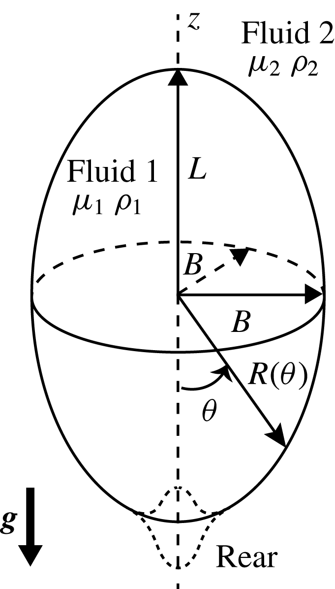
An axisymmetric droplet rising in the quiescent fluid, along the axial (
 $z$
) direction. The fluids inside and outside are labelled as fluid 1 and fluid 2 respectively, so that their dynamic viscosities are
 ${\it\mu}_{1}$
and
 ${\it\mu}_{2}$
and their densities are
 ${\it\rho}_{1}$
and
 ${\it\rho}_{2}$
. The polar coordinates
 $R({\it\theta})$
are used to represent its shape, where
 ${\it\theta}$
is measured from its rear stagnation point;
 $L$
and
 $B$
represent the axis length along the revolution axis and orthogonal directions.

3. Non-modal analysis: theory
As shown by the modal analysis of Kojima et al. (Reference Kojima, Hinch and Acrivos1984), the operator
 $\unicode[STIX]{x1D63C}$
has a stable spectrum with all of its eigenvalues having negative real parts, irrespective of the magnitude of the surface tension, as long as the capillary number is finite. This model analysis predicts the long-term behaviour of the disturbance, but in the short-term limit it is only valid if the linear operator
 $\unicode[STIX]{x1D63C}$
is normal, i.e. its eigenvectors are orthogonal. In the case of a non-normal operator, even though the amplitudes of all eigenmodes decay exponentially, their non-orthogonality can lead to a transient energy growth over a short time. We indeed found that
 $\unicode[STIX]{x1D63C}$
was non-normal. The optimal growth
 $G^{max}$
of the initial energy (
 $L_{2}$
norm) over a chosen time interval
 $[0,T]$
(Schmid Reference Schmid2007) is
 $$\begin{eqnarray}G^{max}(T)=\max _{\boldsymbol{ f}(0)}\left[G(T)=\frac{\Vert \boldsymbol{f}(T)\Vert _{2}}{\Vert \boldsymbol{f}(0)\Vert _{2}}\right]=\Vert \!\exp (T\unicode[STIX]{x1D63C})\Vert _{2},\end{eqnarray}$$
where
 $\boldsymbol{f}(0)$
denotes the initial perturbation.
 $G^{max}(T)$
represents the maximum amplification of the initial energy at a target time (the so-called horizon)
 $T$
where the optimization has been performed over all possible perturbations
 $\boldsymbol{f}(0)$
. The optimal initial perturbation for horizon
 $T$
will be denoted
 $\boldsymbol{f}_{[T]}^{opt}(0)$
. The quantity
 $G^{max}$
is the envelope of all individual gain profiles, indicating the presence of transient growth when
 $G^{max}(T)>1$
for some
 $T$
.
Compared with the
 $L_{2}$
norm in (3.1), it is natural to introduce a physically driven form of energy, designed for the physical problem at hand. In the present study, the variation of surface area of the droplet
 ${\rm\Delta}S$
is chosen as the target energy, since
 ${\it\gamma}{\rm\Delta}S$
indicates the interfacial energy throughout the evolution;
 ${\rm\Delta}S$
is zero only for a spherical droplet and is positive otherwise. The surface area is
 $S=2{\rm\pi}\int _{0}^{{\rm\pi}}R^{2}\sin {\it\theta}\sqrt{1+[(1/R)(\partial R/\partial {\it\theta})]^{2}}\,\text{d}{\it\theta}$
. Assuming small deformation and thus
 $(1/R)(\partial R/\partial {\it\theta})\ll 1$
, a Taylor expansion yields
 $$\begin{eqnarray}S=2{\rm\pi}\int _{0}^{{\rm\pi}}R^{2}\sin {\it\theta}\left(1+\frac{1}{2R^{2}}\left(\frac{\partial R}{\partial {\it\theta}}\right)^{2}\right)\text{d}{\it\theta}.\end{eqnarray}$$
Plugging (2.3) into (3.2), the area variation
 ${\rm\Delta}S=S-4{\rm\pi}$
is found to be
 $$\begin{eqnarray}{\rm\Delta}S/(2{\rm\pi}{\it\delta}^{2})=\boldsymbol{f}^{\text{T}}\unicode[STIX]{x1D648}_{{\rm\Delta}S}\boldsymbol{f}+o({\it\delta}^{2}),\end{eqnarray}$$
where
 $\unicode[STIX]{x1D648}_{{\rm\Delta}S}$
is the so-called weight matrix (Schmid Reference Schmid2001) of size
 $m\times m$
, with entries
 $$\begin{eqnarray}\unicode[STIX]{x1D648}_{{\rm\Delta}S}(i,j)=2{\it\delta}_{ij}^{K}(2i+1)+\frac{1}{2}(2i+1)(2j+1)\int _{0}^{{\rm\pi}}P_{i}^{\prime }(\cos {\it\theta})P_{j}^{\prime }(\cos {\it\theta})\sin ^{3}{\it\theta}\,\text{d}{\it\theta}.\end{eqnarray}$$
The optimal growth of
 ${\rm\Delta}S$
can now be defined as
 $$\begin{eqnarray}G_{{\rm\Delta}S}^{max}(T)=\max _{\boldsymbol{ f}(0)}\left[G_{{\rm\Delta}S}(T)=\frac{\sqrt{{\rm\Delta}S(T)}}{\sqrt{{\rm\Delta}S(0)}}\right]=\max _{\boldsymbol{f}(0)}\left[G_{{\rm\Delta}S}(T)=\frac{\sqrt{\boldsymbol{f}^{\text{T}}\unicode[STIX]{x1D648}_{{\rm\Delta}S}\boldsymbol{ f}}}{\sqrt{\boldsymbol{f}^{\text{T}}(0)\unicode[STIX]{x1D648}_{{\rm\Delta}S}\boldsymbol{ f}(0)}}\right].\end{eqnarray}$$
By Cholesky decomposition
 $\unicode[STIX]{x1D648}_{{\rm\Delta}S}=\unicode[STIX]{x1D641}^{\text{T}}\unicode[STIX]{x1D641}$
, the above equation is formulated as
 $$\begin{eqnarray}G_{{\rm\Delta}S}^{max}(T)=\max _{\boldsymbol{ f}(0)}\left[G_{{\rm\Delta}S}(T)=\frac{\Vert \unicode[STIX]{x1D641}\boldsymbol{f}(T)\Vert _{2}}{\Vert \unicode[STIX]{x1D641}\boldsymbol{f}(0)\Vert _{2}}\right].\end{eqnarray}$$
In a similar way to how the asymptotic stability (
 $t\rightarrow \infty$
) is determined by the eigenvalues of the evolution operator
 $\unicode[STIX]{x1D63C}$
, the maximum instantaneous growth rate of the perturbation energy at
 $t=0^{+}$
can be determined algebraically, expanding the matrix exponential
 $\exp (t\unicode[STIX]{x1D63C})\approx I+t\unicode[STIX]{x1D63C}$
at
 $t=0^{+}$
. The growth rate of the excess area
 ${\rm\Delta}S$
is then
 $$\begin{eqnarray}\frac{1}{{\rm\Delta}S}\left.\frac{\text{d}{\rm\Delta}S}{\text{d}t}\right|_{t=0^{+}}=\frac{\boldsymbol{f}^{\text{T}}(0)[\unicode[STIX]{x1D63C}^{\text{T}}\unicode[STIX]{x1D641}^{\text{T}}\unicode[STIX]{x1D641}+\unicode[STIX]{x1D641}^{\text{T}}\unicode[STIX]{x1D641}\unicode[STIX]{x1D63C}]\boldsymbol{f}(0)}{\boldsymbol{f}^{\text{T}}(0)\unicode[STIX]{x1D641}^{\text{T}}\unicode[STIX]{x1D641}\boldsymbol{f}(0)}.\end{eqnarray}$$
By introducing
 $\boldsymbol{h}=\unicode[STIX]{x1D641}\boldsymbol{f}(0)$
, the maximum growth rate of
 ${\rm\Delta}S$
is formulated as
 $$\begin{eqnarray}\max \frac{1}{{\rm\Delta}S}\left.\frac{\text{d}{\rm\Delta}S}{\text{d}t}\right|_{t=0^{+}}=\max _{\boldsymbol{h}}\frac{\boldsymbol{h}^{\text{T}}[\unicode[STIX]{x1D641}\unicode[STIX]{x1D63C}\unicode[STIX]{x1D641}^{-1}+(\unicode[STIX]{x1D641}\unicode[STIX]{x1D63C}\unicode[STIX]{x1D641}^{-1})^{\text{T}}]\boldsymbol{h}}{\boldsymbol{h}^{\text{T}}\boldsymbol{h}},\end{eqnarray}$$
which becomes the optimization of a Rayleigh quotient with respect to
 $\boldsymbol{h}$
. Because
 $\unicode[STIX]{x1D641}\unicode[STIX]{x1D63C}\unicode[STIX]{x1D641}^{-1}+(\unicode[STIX]{x1D641}\unicode[STIX]{x1D63C}\unicode[STIX]{x1D641}^{-1})^{\text{T}}$
is a symmetric operator, the maximum is given by its largest eigenvalue,
 $$\begin{eqnarray}\displaystyle \max \frac{1}{\sqrt{{\rm\Delta}S}}\left.\frac{\text{d}\sqrt{{\rm\Delta}S}}{\text{d}t}\right|_{t=0^{+}}=s_{max}\left[\frac{1}{2}(\unicode[STIX]{x1D641}\unicode[STIX]{x1D63C}\unicode[STIX]{x1D641}^{-1}+(\unicode[STIX]{x1D641}\unicode[STIX]{x1D63C}\unicode[STIX]{x1D641}^{-1})^{\text{T}})\right], & & \displaystyle\end{eqnarray}$$
where
 $s_{max}[\cdot ]$
denotes the largest eigenvalue. This maximum instantaneous growth rate is commonly called the numerical abscissa (Trefethen & Embree Reference Trefethen and Embree2005), which is closely linked to the numerical range
 $W_{{\rm\Delta}S}(\unicode[STIX]{x1D63C},\unicode[STIX]{x1D641})$
defined as the set of all Rayleigh quotients,
 $$\begin{eqnarray}W_{{\rm\Delta}S}(\unicode[STIX]{x1D63C},\unicode[STIX]{x1D641})\equiv \{z:z=(\unicode[STIX]{x1D641}\unicode[STIX]{x1D63C}\unicode[STIX]{x1D641}^{-1}\boldsymbol{p},\boldsymbol{p})/(\boldsymbol{p},\boldsymbol{p})\}.\end{eqnarray}$$
The numerical range is the convex hull of the spectrum for a normal operator (and is therefore always in the stable half-plane
 $z_{r}<0$
for a stable operator), but can extend significantly to even protrude into the unstable half-plane
 $z_{r}>0$
for stable non-normal operators. Its maximum protrusion is equal to the numerical abscissa and thus determines the maximum energy growth rate at
 $t=0^{+}$
.
4. Non-modal analysis: results
4.1. Transient growth and numerical range
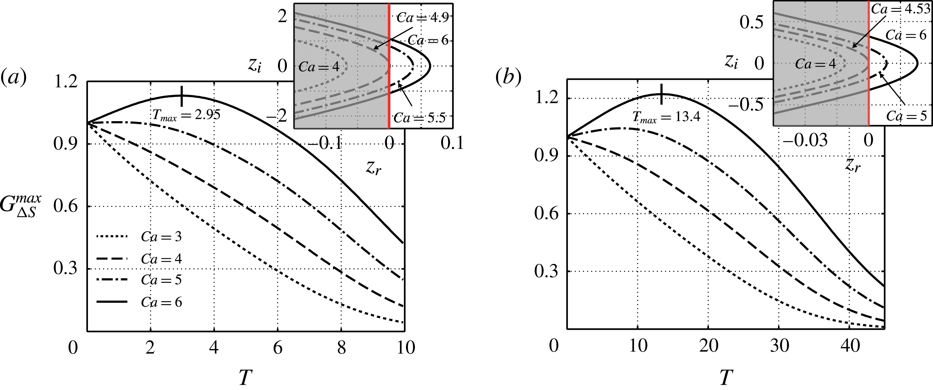
In figure 2, we show the optimal growth of the interfacial energy
 $G_{{\rm\Delta}S}^{max}(T)$
for viscosity ratios of
 ${\it\lambda}=0.5$
and
 $5$
, varying the capillary number
 $\mathit{Ca}$
. The threshold value of
 $\mathit{Ca}$
to yield transient growth is between
 $4$
and
 $5$
, in accordance with the rightmost boundary of the numerical range (see inset) depicted in the complex plane
 $(z_{r},z_{i})$
. The boundary is almost tangent to
 $z_{r}=0$
at
 $\mathit{Ca}\approx 4.9$
for
 ${\it\lambda}=0.5$
and
 $\mathit{Ca}\approx 4.53$
for
 ${\it\lambda}=5$
, representing the critical capillary number
 $\mathit{Ca}_{c}$
above which the maximum energy growth rate at
 $t=0$
,
 $\max _{\boldsymbol{f}(0)}(1/\sqrt{{\rm\Delta}S})(\text{d}\sqrt{{\rm\Delta}S}/\text{d}t)|_{t=0^{+}}$
, is positive, guaranteeing transient growth.
The optimal growth of the interfacial energy
 $G_{{\rm\Delta}S}^{max}(T)$
versus the non-dimensional time
 $T$
, for viscosity ratio
 ${\it\lambda}=0.5$
(a) and
 ${\it\lambda}=5$
(b); for each case, four capillary numbers
 $\mathit{Ca}$
are shown, and for the highest
 $\mathit{Ca}$
, the time
 $T_{max}$
corresponding to the peak energy growth is marked. The inset shows the boundary of the numerical range
 $(z_{r},z_{i})$
.

4.2. Linear growth and shape evolutions
Non-modal analysis not only predicts the maximum energy growth over a particular time interval, but also provides the optimal perturbation, i.e. the initial shape coefficients
 $\boldsymbol{f}_{[T]}^{opt}(0)$
that ensure the optimal gain at horizon
 $T$
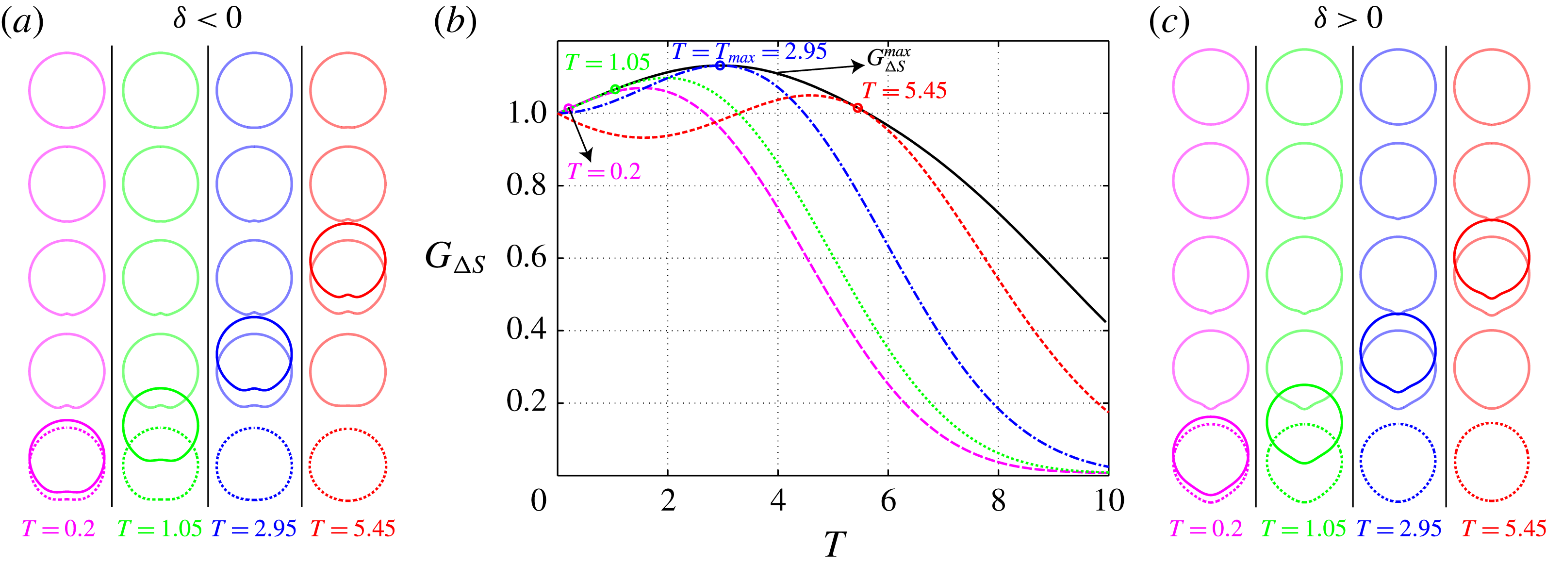
. Figure 3 depicts the individual energy gains
 $G_{{\rm\Delta}S}$
for four optimal initial conditions
 $\boldsymbol{f}_{[T]}^{opt}(0)$
corresponding to
 $T=0.2$
, 1.05, 2.95 and 5.45, with
 ${\it\lambda}=0.5$
and
 $\mathit{Ca}=6$
. Their gain profiles are tangent to
 $G_{{\rm\Delta}S}^{max}(T)$
at
 $t=T$
. The optimal perturbation targeting
 $T=T_{max}=2.95$
coincides with the optimal growth
 $G_{{\rm\Delta}S}^{max}$
at its peak.
Assuming small deformation amplitude and integrating (2.4) in time, the linear shape evolution is readily reconstructed for the droplets with the four optimal initial conditions, depicted in figure 3, at time
 $t=0$
(dashed), 2.5, 5, 7.5, 10 (light solid) and the target time
 $t=T$
(solid); the evolution is shown for negative/positive
 ${\it\delta}$
in (a)/(c). For both signs, the initial perturbation is mainly introduced near the tail (
 ${\it\theta}=0$
) of the droplet where the interface is respectively flattened for
 ${\it\delta}<0$
and stretched for
 ${\it\delta}>0$
while the front part of the droplet remains spherical. In accordance with the modal analysis implying a linearly stable evolution, the perturbations eventually decay and the droplets finally recover a spherical shape.
Linear growth
 $G_{{\rm\Delta}S}$
of the interfacial energy of the droplets with an optimal initial perturbation
 $\boldsymbol{f}_{[T]}^{opt}(0)$
for the target times
 $T=0.2$
, 1.05, 2.95 and 5.45; the solid curve indicates the optimal growth
 $G_{{\rm\Delta}S}^{max}(T)$
and it reaches its peak at
 $T=T_{max}=2.95$
. The linear shape evolution of the perturbations is shown for negative and positive
 ${\it\delta}$
in (a) and (c) respectively.

5. Nonlinear analysis
5.1. Nonlinear energy growth and shape evolution using DNS
As the droplets deform more and more on increasing the initial perturbation amplitude, nonlinearities become significant and the droplet evolution cannot be adequately described by the linearized equations. We resort to DNS to address the nonlinear dynamics using a three-dimensional axisymmetric boundary integral implementation, following the standard approach of Koh & Leal (Reference Koh and Leal1989).
We focus on the droplets of
 ${\it\lambda}=0.5$
and
 $\mathit{Ca}=6$
with the optimal perturbation
 $\boldsymbol{f}_{[T_{max}]}^{opt}(0)$
achieving the peak of the optimal energy growth
 $G_{{\rm\Delta}S}^{max}$
at
 $T_{max}$
. Two slightly different magnitudes of perturbation
 ${\it\delta}=0.0496,0.0505$
are chosen for the positive
 ${\it\delta}$
and similarly
 ${\it\delta}=-0.122,-0.126$
for the negative case. Their energy growth
 $G_{{\rm\Delta}S}(t)=\sqrt{{\rm\Delta}S(t)/{\rm\Delta}S(0)}$
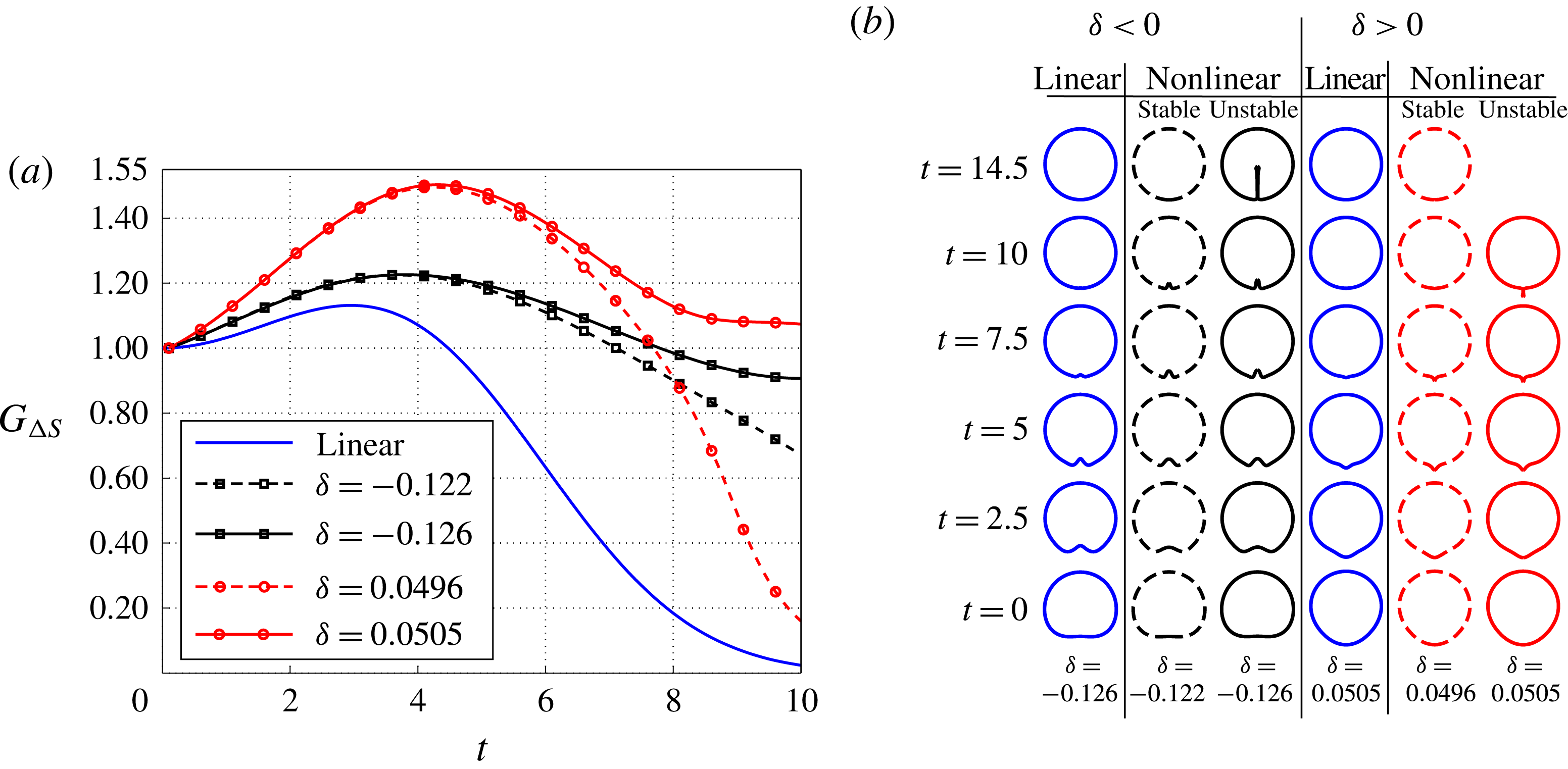
is plotted in figure 4(a), together with the linear counterpart
 $G_{{\rm\Delta}S}(t)$
using (3.3). The linear and nonlinear energy growth share the same trend in the initial growing phase
 $t<3$
, but differ as the former is approximated by a truncated Taylor expansion. For the two values of
 ${\it\delta}$
with the same sign but slightly different magnitude, the energy growth curves almost collapse before reaching their peaks at
 $t\approx 4$
, but diverge afterwards;
 $G_{{\rm\Delta}S}$
decays for the smaller magnitudes
 ${\it\delta}=-0.122$
and
 ${\it\delta}=0.0496$
, indicating stable evolutions, but maintains a sustained value of around
 $1$
for larger initial amplitudes
 ${\it\delta}=-0.126$
and
 ${\it\delta}=0.0505$
, implying the onset of instability.
(a) Nonlinear energy growth
 $G_{{\rm\Delta}S}$
of the droplets with the optimal perturbation
 $\boldsymbol{f}_{[T]}^{opt}(0)$
for the target time
 $T=T_{max}=2.95$
; the solid curve indicates the linear energy growth. For positive
 ${\it\delta}$
,
 $G_{{\rm\Delta}S}$
values for droplets with
 ${\it\delta}=0.0496$
and
 $0.0505$
are shown, the former/latter being stable/unstable; for negative
 ${\it\delta}$
, the chosen values leading to stable and unstable evolution are
 ${\it\delta}=-0.122$
and
 ${\it\delta}=-0.126$
respectively. (b) The shape evolutions of the corresponding droplets.

The shape evolutions of droplets are shown in figure 4(b). For
 ${\it\delta}=-0.122$
and
 $-0.126$
, no significant difference is observed for
 $0<t<7.5$
: an inward cavity develops at the rear and sharpens; it is subsequently smoothed out and disappears for
 ${\it\delta}=-0.122$
, while it keeps growing to form a long indentation for
 ${\it\delta}=-0.126$
. These two values of
 ${\it\delta}$
bound a threshold initial amplitude required to excite nonlinear instabilities. A similar trend is found for positive values of
 ${\it\delta}$
, while the instability arises through the formation of a dripping tail.
It becomes natural to introduce
 ${\it\delta}_{c}$
, the critical magnitude of the perturbation above/below which the evolution of the drop is unstable/stable. Parametric computations are conducted to identify
 ${\it\delta}_{c}^{\pm }$
within a confidence interval (for instance
 ${\it\delta}_{c}^{+}\in [0.0496,0.0505]$
and
 ${\it\delta}_{c}^{-}\in [-0.122,-0.126]$
as in figure 4(a)). Searching in both directions, the critical amplitude is then defined as
 ${\it\delta}_{c}=\min (|{\it\delta}_{c}^{+}|,|{\it\delta}_{c}^{-}|)$
. When
 ${\it\lambda}=0.5$
and
 $\mathit{Ca}=6$
,
 $|{\it\delta}_{c}^{-}|>|{\it\delta}_{c}^{+}|$
, implying that the instability tends to favour an initially stretched tail with respect to a flattened bottom; otherwise when
 ${\it\lambda}=5$
the situation reverses
 $(|{\it\delta}_{c}^{-}|<|{\it\delta}_{c}^{+}|)$
, as discussed in the next section.
5.2. Critical amplitude of the perturbation
 ${\it\delta}_{c}$

Following the description of the previous paragraph, the critical deformation amplitude
 ${\it\delta}_{c}(T)$
can be determined for any targeting time
 $T$
and associated optimal initial perturbation
 $\boldsymbol{f}_{[T]}^{opt}(0)$
. The critical deformation amplitude
 ${\it\delta}_{c}(T)$
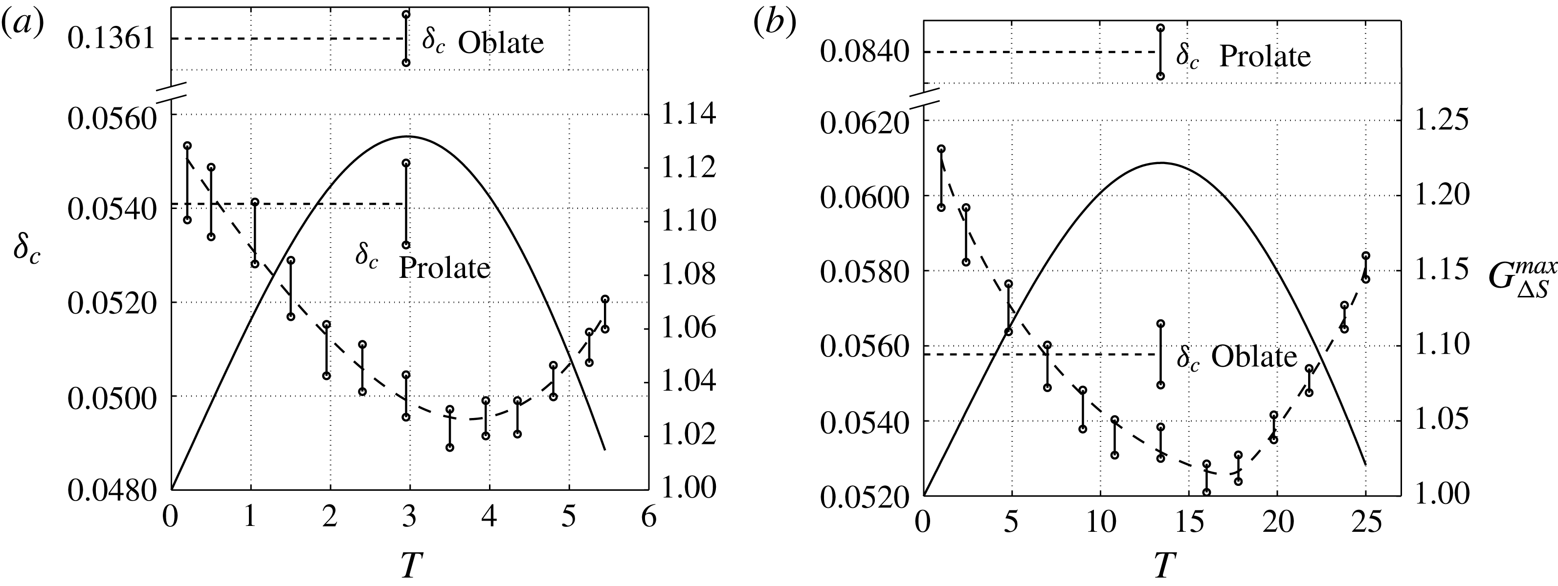
is plotted in figure 5 for
 $\mathit{Ca}=6$
and both
 ${\it\lambda}=0.5$
and
 ${\it\lambda}=5$
, together with the optimal growth
 $G_{{\rm\Delta}S}^{max}$
. The critical deformation amplitude
 ${\it\delta}_{c}$
is negatively correlated with
 $G_{{\rm\Delta}S}^{max}$
and corresponds to a target time
 $T$
slightly larger than
 $T_{max}$
where the peak transient growth is reached. This shows that the transient growth reduces the threshold nonlinearity needed to trigger instabilities and consequently the critical magnitude of the initial perturbation.
We also determined the critical amplitude
 ${\it\delta}_{c}^{P/O}$
for an initially prolate (
 $\text{P}$
)/oblate (
 $\text{O}$
) ellipsoidal droplet to be unstable, as reported in figure 5. When the fluid inside the droplet is less viscous than the one outside, i.e.
 ${\it\lambda}<1$
, an initially prolate droplet is more unstable,
 ${\it\delta}_{c}^{P}$
is less than half that of an oblate droplet
 ${\it\delta}_{c}^{O}$
; the trend reverses as
 ${\it\lambda}>1$
. Such an observation is in agreement with the results of Koh & Leal (Reference Koh and Leal1989) using DNS (see figure 11 of their paper). As expected, the minimum
 ${\it\delta}_{c}$
using the optimal perturbations is smaller than
 $\min ({\it\delta}_{c}^{P},{\it\delta}_{c}^{O})$
based on the limited family of ellipsoidal shapes.
The critical perturbation magnitude
 ${\it\delta}_{c}$
for (a)
 $({\it\lambda},\mathit{Ca})=(0.5,6)$
and (b)
 $({\it\lambda},\mathit{Ca})=(5,6)$
. The upper and lower limits of
 ${\it\delta}_{c}$
(measured by the left scale) are plotted versus the target time
 $T$
, with a curve fitted to show the trend. Accordingly, the linear energy growth
 $G_{{\rm\Delta}S}^{max}$
(measured by the right scale) is provided. Here,
 ${\it\delta}_{c}^{P}$
and
 ${\it\delta}_{c}^{O}$
are the critical magnitudes for initially prolate and oblate droplets respectively.

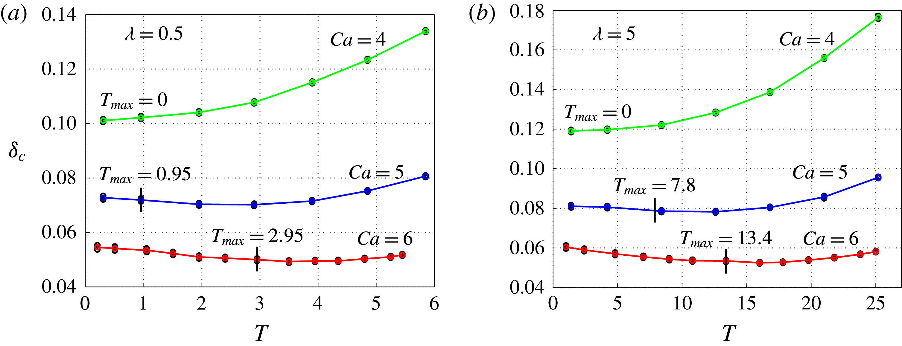
So far, we have analysed the critical amplitude
 ${\it\delta}_{c}$
of perturbations exhibiting transient energy growth. We would like to know how it varies as the transient growth decreases and even disappears as it is suppressed by high surface tension. In addition to
 $\mathit{Ca}=6$
, the time dependence of
 ${\it\delta}_{c}$
is shown in figure 6 for
 $\mathit{Ca}=4,5$
. As expected,
 ${\it\delta}_{c}$
increases with decreasing
 $\mathit{Ca}$
, by a factor of approximately
 $3$
, varying from the highest to the lowest
 $\mathit{Ca}$
. With respect to
 $T$
,
 ${\it\delta}_{c}$
varies non-monotonically for
 $\mathit{Ca}=5,6$
, showing transient growth. In the absence of transient growth, like for
 $\mathit{Ca}=4$
,
 ${\it\delta}_{c}$
increases with
 $T$
monotonically. Indeed, without transient growth, the energy decays monotonically and
 $T_{max}=0$
, hence the minimum
 ${\it\delta}_{c}$
appears at
 $T\approx 0$
.
Akin to figure 5, adding the
 ${\it\delta}_{c}$
for two smaller values of
 $\mathit{Ca}$
for (a)
 ${\it\lambda}=0.5$
and (b)
 ${\it\lambda}=5$
.

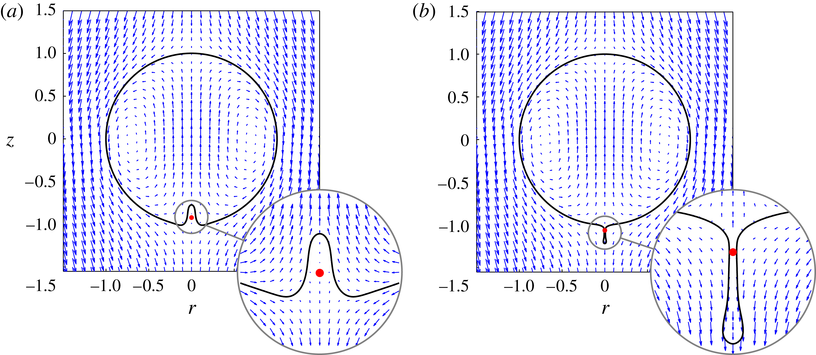
The flow field co-moving with the droplet, using the optimal initial coefficient
 $\boldsymbol{f}_{[T_{max}]}^{opt}(0)$
, when
 $({\it\lambda},\mathit{Ca})=(0.5,6)$
, (a)
 ${\it\delta}=-0.126$
and (b)
 ${\it\delta}=0.0505$
. The red dot indicates the stagnation point of the flow.

6. Conclusion and discussion
In this paper, we have performed non-modal analysis and DNS to investigate the shape instabilities of an inertialess rising droplet which tends to recover the spherical shape, the attractor solution, due to surface tension. For sufficiently low surface tension, transient growth of the interfacial energy arises and leads to a bypass transition. This reduces the initial disturbance amplitude required to trigger instability, hence significantly decreasing the threshold magnitude of perturbation for the droplet to escape the basin of attraction. This magnitude is negatively correlated to the optimal growth of the interfacial energy.
We now compare our results with the work of Koh & Leal (Reference Koh and Leal1989) who employed DNS to identify the critical capillary number
 $\mathit{Ca}_{c}$
leading to shape instabilities of an initially prolate or oblate ellipsoidal rising droplet; the magnitude of perturbation is
 ${\it\Delta}=(L-B)/(L+B)$
(see figure 1). For their lowest magnitude
 $|{\it\Delta}|=1/21$
considered,
 $\mathit{Ca}_{c}\in (4,5)$
for
 ${\it\lambda}=0.1,0.5$
and
 $5$
, indeed close to our prediction:
 $\mathit{Ca}_{c}\approx 5.42$
, 4.9 and 4.53 respectively for the same
 ${\it\lambda}$
. Additionally, Koh & Leal (Reference Koh and Leal1989) observed that for a viscosity ratio
 ${\it\lambda}<1/{\it\lambda}>1$
, the first unstable pattern appears as a protrusion/indentation developing near the tail of the droplet that is initially a prolate/oblate. The trend holds in our case even though we search over all possibilities for the most ‘dangerous’ initial perturbation instead of using an initially ellipsoidal shape. This is also reflected from the initial shapes: as
 ${\it\lambda}<1/{\it\lambda}>1$
, the optimal shape shares a common feature with an oblate/prolate ellipsoid, namely its rear interface is compressed/stretched.
To explain the dependence of the instability patterns on the viscosity ratio
 ${\it\lambda}$
, let us focus on the velocity field near the tail of the droplet (see figure 7), where the flow resembles a uniaxial extensional flow, drawing the tip into the drop on the top side and pulling it outwards on the other side. We suggest that this imbalance induces the onset of the shape instability. The internal (respectively external) viscous force on the tip is
 ${\it\mu}_{1}\partial u_{z}^{tip}/\partial z$
(respectively
 ${\it\mu}_{2}\partial u_{z}^{tip}/\partial z$
). When
 ${\it\mu}_{1}<{\it\mu}_{2}$
, i.e.
 ${\it\lambda}<1$
, the external viscous effect overcomes the internal one, hence the perturbation tends to be stretched outward to form a protrusion; otherwise, when
 ${\it\lambda}>1$
, it is prone to be sucked inwards to form an indentation.
Developed originally for hydrodynamic stability analysis, non-modal tools have here demonstrated the predictive capacity for the inertialess shape instabilities of capillary interfaces. This work might stimulate the application of non-modal analysis for complex multiphase flow instabilities even at low Reynolds numbers.
Acknowledgement
L.Z. thanks F. Viola for the helpful discussions. We thank the anonymous referee for pointing out an incorrect coefficient in our previous derivation. Computer time from SCITAS at EPFL is acknowledged, and the European Research Council is acknowledged for funding the work through a starting grant (ERC SimCoMiCs 280117).