3.1. Calculation cases and validity verification

In this paper, the flow around an equal straight circular cylinder is numerically simulated under the conditions of $Ma=0.2$ and $Re=3900$ . This Reynolds number is within the subcritical flow range, which is characterised by the laminar boundary layer on the cylinder wall, the flow separation on the upper and lower sides of the cylinder and the transition to turbulence in the separated shear layer. In order to obtain detailed flow-field results and avoid the high computational cost of direct numerical simulation, LES is used to obtain flow-field data in this paper. The WALE model (Nicoud & Ducros Reference Nicoud and Ducros1999) is designed to minimise the influence of the model when calculating the laminar boundary layer, which is very important for flows that contain both laminar and turbulent flows, as it ensures accurate prediction of the boundary layer. As a result, the WALE model is selected for the working conditions studied in this paper. In this paper, the spatial discretisation of the convective terms is performed using the HLLC scheme, while the viscous terms are discretised using the DDG scheme. The time discretisation is based on an implicit Runge–Kutta method.

Figure 1.

Diagram of the computational domain.

Figure 1 shows a diagram of the computational domain, where $D$ is the diameter of the cylinder and the origin of the coordinates is located at the centre of the cylinder. The spanwise length of the cylinder is selected as $\pi D$ . The upstream and downstream boundaries are $12D$ and $24D$ away from the centre of the cylinder, and the top and bottom boundaries are both $12D$ away from the centre of the cylinder. The wall is subject to a no-slip condition and is applied as a periodic boundary condition in the spanwise direction. The remaining surfaces of the computational domain are set to far-field boundary conditions.

Figure 2.

Comparison of capturing the Q-criterion structure on the XOZ plane with different grid numbers. From (a–e), the cases are ordered from CASE1 to CASE5.

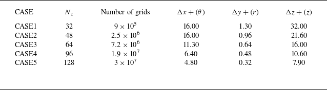
Since the sound source term mainly originates from the gradient in the flow field, the accuracy of capturing the gradient will directly determine the precision of capturing the sound source structure. Figure 2 shows a comparison of the capture of flow structures under different grid numbers, and table 1 lists the parameters for each grid set-up. The term $0.5({\left |\boldsymbol{\varOmega }\right |}_{F}+{\left |\boldsymbol{D}\right |}_{F})$ is employed to visualise the flow-field structure, where $\boldsymbol{D}$ is the symmetric tensor obtained from the Cauchy–Stokes decomposition of the velocity tensor $\boldsymbol{A}$ , $\boldsymbol{\varOmega }$ is the antisymmetric tensor resulting from the same decomposition and ${ |\dots |}_{F}$ denotes the Frobenius norm. This is the definition of the $Q$ criterion (Jeong & Hussain Reference Jeong and Hussain1995). Its expression encompasses the nonlinear effects of each term of the velocity gradient, making it suitable for representing the capture of the gradient. From the results, it is evident that there is a significant difference in the ability of different grids to capture flow structures. Given the need for precise capture of the sound source and flow structure, this paper ultimately adopts the finest grid, namely CASE5.

Table 1.

Specific parameters of different sets of grids, where $\theta$ is the coordinate in the circumferential direction, $r$ is the coordinate in the radial direction and $z$ is the coordinate in the spanwise direction.

Figure 3 shows a schematic diagram of the computational grid distribution. The grid is structured using hexahedral elements. Based on the areas of focus in this study, the grid distribution is highly concentrated near the cylindrical surface and in the near wake. In view of the mesh resolution requirements near the wall, the boundary-layer mesh was refined to resolve the viscous sublayer near the wall, ensuring that the wall $y+$ is less than 1. The finer mesh improves spatial resolution and can capture finer-scale turbulent structures. To meet the requirements of LES, the time step must be adjusted to accommodate the evolution and convection of these finer structures. To ensure temporal resolution, the dimensionless time step of this simulation is $\Delta {t}^{\ast }=0.00069$ . Flow sampling begins after the flow reaches periodic stability, and a result is extracted every one time step. The sampling time is 0.1 s, corresponding to approximately 140 vortex-shedding cycles.

Figure 3.

Computational grid diagram. (a) Diagram of the XYplane grid near the cylindrical wall. (b) Diagram of the spanwise grid on the cylindrical wall surface.

Table 2.

Comparison of main flow quantities. Here $St={f}_{vs}D/U_0$ , ${C_d} = Dra/(0.5{\rho _0 }U_0 ^2S)$ , ${C_l} = Lif/(0.5{\rho _0 }U_0 ^2S)$ , ${f}_{vs}$ is the vortex shedding frequency, $D$ the cylinder diameter, $U_0$ the free-stream velocity, $\rho _0$ the density of the free stream, $Dra$ the drag forces, $Lif$ the lift forces and $S$ the characteristic area (Lourenco & Shih Reference Lourenco and Shih1994; Fröhlich et al. Reference Fröhlich, Rodi, Kessler, Parpais, Bertoglio and Laurence1998; Norberg Reference Norberg1998; Dong et al. Reference Dong, Karniadakis, Ekmekci and Rockwell2006; Parnaudeau et al. Reference Parnaudeau, Carlier, Heitz and Lamballais2008; Kahil Reference Kahil2011; Aguedal et al. Reference Aguedal, Semmar, Berrouk, Azzi and Oualli2018).

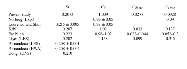
In order to verify the validity of the numerical simulation flow results, we use experiments and other simulation results as benchmarks for numerical verification. First, the force characteristics of the cylinder and the Strouhal number are quantitatively compared. Table 2 shows the comparison of the time-averaged and fluctuating root-mean-square (RMS) values of the aerodynamic forces obtained in this paper with the experimental and other numerical studies. The average drag coefficient in this paper is 1.009, which is within the range of experimental results. Previous numerical studies have shown that the RMS values of the lift coefficient and the drag coefficient are very sensitive to the turbulence model and the grid resolution. In the simulation of this paper, the RMS values of the drag coefficient and the lift coefficient are 0.0277 and 0.0928, respectively, which are slightly different from the results of other studies, but within a reasonable range. The Strouhal number of the numerical simulation in this paper is 0.2073, which is in good agreement with the experimental and numerical results.

Figure 4 shows the time-averaged pressure coefficient ( ${C}{p}$ ) distribution along the cylinder surface compared with experimental and other LES results (Norberg Reference Norberg1998; Aguedal et al. Reference Aguedal, Semmar, Berrouk, Azzi and Oualli2018), where ${C}{p}=(p-{p}_{0})/(0.5{\rho }_{0}{{U}_{0}}^{2})$ and ${p}_{0}$ is the pressure of the free flow. The results are in good agreement with the experimental data, and although there are slight discrepancies, they are within a reasonable range.

Figure 4.

The comparison of time-averaged pressure coefficients on the cylindrical wall.

Figure 5(a) shows the time-averaged flow velocity profile at different downstream locations ( $X/D = 1.06, 1.54, 2.02$ ) compared with experimental and numerical results (Lourenco & Shih Reference Lourenco and Shih1994; Ma, Karamanos & Karniadakis Reference Ma, Karamanos and Karniadakis2000; Parnaudeau et al. Reference Parnaudeau, Carlier, Heitz and Lamballais2008). Figure 5(b) shows the time-averaged normal velocity profile at different downstream locations ( $X/D = 1.06, 1.54, 2.02$ ) compared with experimental and numerical results. The simulated flow velocity is in good agreement with the previous experimental data.

Figure 5.

The comparison of time-averaged velocity at different downstream locations. (a) Time-averaged streamwise velocity. (b) Time-averaged normal velocity.

In addition, the unsteady results of the numerical simulation are verified through comparison. Figure 6 shows the variance of the streamwise velocity fluctuation and the normal velocity fluctuation at different positions in the wake, compared with experimental and numerical results. In general, the numerical simulation results in this paper are highly consistent with the results of experiments and other numerical studies. When $X/D=1.06$ , figure 6(a) captures two obvious peaks, which are primarily caused by the shear layer. As the distance from the cylinder increases, there is a slight difference in capturing the peaks, which is attributed to the sparse grid in the downstream direction.

Figure 6.

The comparison of velocity fluctuations at different downstream locations. (a) Variance of the streamwise velocity fluctuations. (b) Variance of the normal velocity fluctuations.

3.2. Basic flow field

In order to study the sound source mechanism of the flow around the cylinder, this section first analyses the basic flow structure within the flow field.

Figure 7.

(a) The time-averaged Mach number. (b) The time-averaged vorticity distribution.

Figures 7(a) and 7(b) show the time-averaged Mach number and time-averaged vorticity distribution, respectively. It can be seen that after the incoming flow contacts the cylinder, the fluid is separated on the upper and lower sides and accelerated. An obvious shear-layer structure forms on the upper and lower sides of the cylinder (marked by the blue dashed box), but as it evolves downstream, this distinct structure is gradually destroyed (marked by the red dashed box). Figures 8(a) and 8(b) show the distribution of the time-averaged $X$ velocity component and $Y$ velocity component at different positions in the wake region, respectively. It can be seen that there is an obvious low-speed recirculation area behind the cylinder, which forms a large velocity gradient with the incoming flow velocity. The area with large velocity changes can be clearly captured in figure 8(a), which is also the area where the shear layer is formed. As it develops downstream, the velocity difference between the recirculation area and the outside gradually decreases, the velocity gradient that maintains the shear-layer structure diminishes and the shear layer begins to break apart.

Figure 8.

The distribution of the (a) time-averaged X velocity component (b) time-averaged Y velocity component at different downstream locations. The time-averaged streamline diagram is shown in the inset, in which the grey area represents the cylinder.

Figure 9.

Spatial evolution of velocity fluctuation ( $\langle {u}^{\prime } {u}^{\prime } \rangle$ , $\langle {v}^{\prime } {v}^{\prime }\rangle$ , $\langle {w}^{\prime } {w}^{\prime }\rangle$ ) along the flow direction in the shear layer.

Figure 9 shows the spatial evolution of velocity fluctuations along the flow direction on the shear layer, with the spatial span encompassing the entire shear layer. It can be seen that as the shear-layer structure develops downstream, the fluctuation gradually increases, the stable structure becomes increasingly unstable and eventually breaks into a chaotic vortex zone, where the fluctuation of physical quantities becomes significant. Figure 10 shows the near-field vortex structure generated by the flow around a cylinder. The vortex structure is captured using the $Q$ criterion, with the $Q$ value made dimensionless by ${({c}_{0}/D)}^{2}$ , at values of 0.08 (figure 10 a) and 0.5 (figure 10 b). It can be observed in the figure that the vortex forms near the cylinder and then dissipates, gradually diffusing as it moves. The source of this process originates from the shear layer formed by the interaction between the incoming flow and the wall, which then breaks into many small and chaotic vortex structures with the backflow. Another part forms a wake-shedding vortex that evolves into the far field. The vortex shedding at a Reynolds number of 3900 differs from the paired, alternating, antisymmetric vortices with opposite rotation directions typically generated at low Reynolds numbers. Instead, multiple vortices of different sizes are shed, with each vortex generation and shedding process being distinct. This process is random and also exhibits a significant three-dimensional effect.

Figure 10.

Vortex structure generated by the flow around a cylinder. Vortex structure captured by the Q criterion: Q = 0.08 (a) and Q = 0.5 (b), coloured by Mach number.

The results show that several important flow structures or regions exist in the wake of the cylinder. For ease of description, the flow field can be divided into several regions as shown in figure 11. Region I is the shear layer formed on the upper and lower sides of the cylinder, referred to as the shear layer; region II is the recirculation area near the cylinder, where the vortex is more turbulent, known as the recirculation flow; region III is the wake vortex area where the shed vortex enters the wake and extends to the far field, called the wake vortex. The wall facing the incoming flow in front of the cylinder is called the leading edge, while the wall on the opposite side, which contacts the recirculation zone, is called the leeward side.

Figure 11.

Diagram of the division of different areas.

The complex flow in the cylinder wake originates from the flow separation on the upper and lower sides of the cylinder. The wall behaviour of the flow separation phenomenon is analysed, and figure 12 shows the limiting streamline of the cylinder. It can be observed that the fluid boundary layer, initially adhering closely to the wall, begins to separate from the wall at a certain point and no longer stays attached. This point is referred to as the separation point. A turbulent recirculation area appears after the separation point. Figure 13 shows the surface friction coefficient ( ${c}_{f}$ ) along the surface of the cylinder. The ${c}_{f}$ is related to the shear stress between the fluid and the solid surface, and it characterises the interaction between the fluid and the solid wall due to viscosity. The ${c}_{f}$ is close to 0, indicating that the boundary layer at this position is no longer attached to the wall, and the interaction between the fluid and the wall is weak. To a certain extent, it can characterise the location where the flow separation occurs. The separation point calculated in this paper is about ${87}^{\circ }$ , which is close to the experimental results of Parnaudeau et al. (Reference Parnaudeau, Carlier, Heitz and Lamballais2008) ( ${88}^{\circ }$ ) and the LES results of Breuer (Reference Breuer1998) ( ${87}^{\circ }$ ). Separation is an important flow phenomenon on the cylindrical wall, and the separation point is one of the sources of flow complexity. The subsequent analysis of VTP and SLP on the wall is inseparable from separation, as separation on the wall is closely related to noise.

Figure 12.

The distribution of limiting streamlines on the cylindrical surface. The inset shows the $XY$ plane streamlines near the separation point in the near-wall region. The streamlines are coloured by velocity.

Figure 13.

Surface friction coefficient ${C}_{f}$ along the surface of the cylinder. The point where ${C}_{f}$ is close to 0 is marked as separation point.

Figure 14.

Distribution of the RMS of pressure fluctuations in the wake of a circular cylinder.

Figure 15.

(a) Distribution of pressure fluctuations along the Ydirection at different downstream positions in the wake of a circular cylinder. The vertical axis represents the RMS value of pressure fluctuations. (b) Distribution of pressure fluctuations along the Xdirection on the centreline downstream of the circular cylinder. The vertical axis represents the RMS value of pressure fluctuations.

Figure 14 illustrates the concentrated regions of pressure fluctuations in the wake, while figure 15 quantifies the distribution of the RMS of pressure fluctuations. It is evident that the RMS of pressure fluctuations exhibits a pronounced high-value band downstream of the cylinder trailing edge, with peak values concentrated near the recirculation zone following shear-layer breakdown. Along the streamwise direction, the pressure fluctuations reach their maximum between $X=2D$ and $X=4D$ , after which they gradually decay further downstream. This indicates that the energy of the pressure fluctuations is primarily derived from the complex vortex generation process within the recirculation zone. Furthermore, the pressure fluctuations display a symmetric distribution along the Y axis, with two distinct local peaks in the concentrated regions. This symmetry arises from the periodic pressure fluctuations induced by alternating vortex shedding from the upper and lower shear layers near the wall. The regions of concentrated pressure fluctuations reflect the intensity of local pressure disturbances in the flow field; however, their essence lies in being the final outcome of acoustic variables resulting from the evolution of flow structures such as vortex shedding. In the flow around a circular cylinder, wall pressure fluctuations serve as an important indicator of the interaction between the flow and the cylinder surface. Their distribution characteristics reflect the dynamic effects of key flow structures, such as the separated shear layer, vortex shedding and wake region. Figure 16 shows the distribution of the RMS of pressure fluctuations on the unwrapped cylinder wall. It can be observed that in the leading-edge region, where complex flow structures are absent, the pressure fluctuations are comparatively small. From the leading edge to the upper and lower sides of the cylinder, the pressure fluctuations exhibit a well-organised increasing trend. In contrast, in the trailing-edge region, the pressure fluctuations decrease from their peak values and display a more disordered distribution statistically.

Figure 17 presents the circumferential distribution of the RMS of pressure fluctuations on the cylinder wall. The results reveal that the RMS of pressure fluctuations reaches its peak near the separation point, which is induced by the instability of the separated shear layer. Compared with the region near the leading edge, where flow separation does not occur, the pressure fluctuations on the leeward side of the cylinder also show significant magnitudes, indicating strong flow–wall interactions in these areas.

Figure 16.

Distribution of the RMS of pressure fluctuations on the cylinder wall. The two-dimensional plane represents the angle–Z plane, obtained by unwrapping the cylinder wall with the Zaxis as the fixed axis.

Figure 17.

Circumferential distribution of the RMS of pressure fluctuations on the cylinder wall. Here SP denotes the separation point, and the black dashed line marks the corresponding horizontal coordinate position of the separation point.

3.3. Vortex sound theory: Lamb vector divergence source

Before analysing the sound source based on LTD, this section first discusses the Lamb vector divergence, which is widely used for sound source identification, as a comparison. Compared with the Lighthill source, the Lamb vector divergence, which is more physical and intuitive in relation to vortex motion, is the focus of this section. This section primarily studies the distribution of Lamb vector divergence sound sources in the flow around a cylinder and further explores the physical meaning of Lamb vector divergence under decomposition.

Figure 18.

Distribution of Lamb vector divergence at the wake of a cylinder. The three XY planes shown are at $Z = 0.5D$ , $Z = {\pi }D/2$ and $Z = (\pi - 0.5)D$ , respectively. The cylinder is transparent.

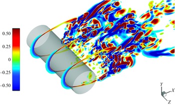
Figure 18 shows the distribution of Lamb vector divergence in the wake of the cylinder. The figure illustrates that the Lamb vector divergence is associated with the shear layer, vortex shedding and swirling flow near the wall induced by backflow–wall interaction. Under the action of the shear flow formed by flow separation, the Lamb vector divergence near the upper and lower shear layers of the cylinder exhibits a strong and stable positive–negative structure. This structure begins to break down as it moves away from the cylinder, and the larger-scale Lamb vector divergence structure gradually becomes discrete into smaller-scale structures. In the recirculation flow, due to secondary backflow–wall interaction, the Lamb vector divergence presents a small and turbulent strip-like structure. The Lamb vector divergence is mathematically a purely kinematic quantity composed of velocity gradients, so the spatial distribution pattern of the Lamb vector divergence is related to the spatial gradient distribution of the physical quantity. Figure 19 shows the distribution of the time-averaged Lamb vector divergence along the $Y$ direction at different downstream locations, made dimensionless using ${({c}_{0}/D)}^{2}$ . It can be observed that the Lamb vector divergence exhibits a positive and a negative peak distribution at the shear layer, where the streamwise velocity gradient along the $Y$ direction reaches a local maximum. As the flow moves away from the cylinder, the peaks gradually flatten, and the shear layer begins to break down.

Figure 19.

The distribution of the time-averaged Lamb vector divergence along the Y direction at different downstream locations. The black dashed line shows the distribution of $\partial u/\partial y$ . The time-averaged velocity distribution and time-averaged streamlines are shown in the inset.

Next, we discuss the mathematical properties and physical interpretation of Lamb vector divergence. Hamman, Klewicki & Kirby (Reference Hamman, Klewicki and Kirby2008) decomposed the Lamb vector divergence as shown in (2.15), indicating that the Lamb vector divergence can be decomposed into two terms, namely the flexion production ${\boldsymbol{u}} {\,\boldsymbol\cdot\,} (\nabla \times {\boldsymbol{\omega }})$ and enstrophy ${\boldsymbol{\omega }} {\,\boldsymbol\cdot\,} {\boldsymbol{\omega }}$ , where the enstrophy term is non-negative. For any vortex flow, the contribution of the enstrophy term to the Lamb vector divergence is always negative. Figures 20(a) and 20(b) show the spatial distribution of ${\boldsymbol{u}} {\,\boldsymbol\cdot\,} (\nabla \times {\boldsymbol{\omega }})$ and ${\boldsymbol{\omega }} {\,\boldsymbol\cdot\,} {\boldsymbol{\omega }}$ , respectively. It can be observed that the alternating positive and negative characteristics of the Lamb vector divergence are only contributed by ${\boldsymbol{u}}{\,\boldsymbol\cdot\,} (\nabla \times {\boldsymbol{\omega }})$ . Figures 21(a) and 21(b) show the spatial distribution of each term of (3.1), respectively, and use ${({c}_{0}/D)}^{2}$ to make them dimensionless. It can be observed that the contributions of ${\boldsymbol{u}} {\,\boldsymbol\cdot\,} (\nabla \times {\boldsymbol{\omega }})$ and ${\boldsymbol{\omega }} {\,\boldsymbol\cdot\,} {\boldsymbol{\omega }}$ are of the same magnitude, and neither term can be neglected. Enstrophy ${\boldsymbol{\omega }} {\,\boldsymbol\cdot\,} {\boldsymbol{\omega }}$ often contributes less when ${\boldsymbol{u}} {\,\boldsymbol\cdot\,} (\nabla \times {\boldsymbol{\omega }})$ reaches the maximum positive value. At this point, the positive value of the Lamb vector divergence is primarily dominated by ${\boldsymbol{u}} {\,\boldsymbol\cdot\,} (\nabla \times {\boldsymbol{\omega }})$ ; however, when ${\boldsymbol{u}} {\,\boldsymbol\cdot\,} (\nabla \times {\boldsymbol{\omega }})$ produces a negative value, the negative contribution from ${\boldsymbol{\omega }} {\,\boldsymbol\cdot\,} {\boldsymbol{\omega }}$ increases, which together leads to the negative value of the Lamb vector divergence:

(3.1) \begin{equation} \nabla {\,\boldsymbol\cdot\,} ({\boldsymbol{\omega }} \times {\boldsymbol{u}}) = {\boldsymbol{u}} {\,\boldsymbol\cdot\,} \nabla \times {\boldsymbol{\omega }} - {\boldsymbol{\omega }} {\,\boldsymbol\cdot\,} {\boldsymbol{\omega }}. \end{equation}

Figure 20.

The spatial instantaneous distribution of (a) ${\boldsymbol{\omega }} {\,\boldsymbol\cdot\,} {\boldsymbol{\omega }}$ and (b) ${\boldsymbol{u}} {\,\boldsymbol\cdot\,} (\nabla \times {\boldsymbol{\omega }})$ . The red region represents positive values and the blue region represents negative values.

Figure 21.

(a,b) The spatial instantaneous distribution of $\nabla {\,\boldsymbol\cdot\,} ( {{\boldsymbol{\omega }} \times {\boldsymbol{u}}} )$ , ${\boldsymbol{\omega }} {\,\boldsymbol\cdot\,} {\boldsymbol{\omega }}$ and ${\boldsymbol{u}} {\,\boldsymbol\cdot\,} (\nabla \times {\boldsymbol{\omega }})$ .

The ${\boldsymbol{\omega }} {\,\boldsymbol\cdot\,} {\boldsymbol{\omega }}$ characterises the presence and intensity of rotation within a certain region and can be considered as the accumulation of regional rotational intensity. The positive area of the Lamb vector divergence represents the accumulation of these rotational intensities. Figure 22 shows the effects of $-{\boldsymbol{\omega }} {\,\boldsymbol\cdot\,} {\boldsymbol{\omega }}$ , ${\boldsymbol{u}} {\,\boldsymbol\cdot\,} (\nabla \times {\boldsymbol{\omega }})$ and $\nabla {\,\boldsymbol\cdot\,} ( {{\boldsymbol{\omega }} \times {\boldsymbol{u}}} )$ . Red represents the accumulation effect of rotational intensity ${\boldsymbol{\omega }} {\,\boldsymbol\cdot\,} {\boldsymbol{\omega }}$ , while blue represents the consumption effect of rotational intensity due to ${\boldsymbol{u}} {\,\boldsymbol\cdot\,} (\nabla \times {\boldsymbol{\omega }})$ . The physical characteristic of the Lamb vector divergence is the effect of the rotational strength stored in the flow after it has been consumed by flexion production.

Figure 22.

Schematic diagram of the effects of $\nabla {\,\boldsymbol\cdot\,} ({\boldsymbol{\omega }} \times {\boldsymbol{u}})$ , ${\boldsymbol{\omega }} {\,\boldsymbol\cdot\,} {\boldsymbol{\omega }}$ and ${\boldsymbol{u}} {\,\boldsymbol\cdot\,} (\nabla \times {\boldsymbol{\omega }})$ .

On further decomposition of ${\boldsymbol{u}} {\,\boldsymbol\cdot\,} (\nabla \times {\boldsymbol{\omega }})$ , one can obtain

(3.2) \begin{equation} {\boldsymbol{u}} {\,\boldsymbol\cdot\,} (\nabla \times {\boldsymbol{\omega }}) = {\boldsymbol{u}} {\,\boldsymbol\cdot\,} (\nabla \vartheta ) - {\boldsymbol{u}} {\,\boldsymbol\cdot\,} {\nabla ^2}{\boldsymbol{u}}, \end{equation}

where ${\boldsymbol{u}} {\,\boldsymbol\cdot\,} (\nabla \vartheta )$ is related to the compressibility effect and ${\boldsymbol{u}} {\,\boldsymbol\cdot\,} {\nabla ^2}{\boldsymbol{u}}$ can be written as

(3.3) \begin{eqnarray} {\boldsymbol{u}} {\,\boldsymbol\cdot\,} {\nabla ^2}{\boldsymbol{u}} = {u_i}{u_{i,jj}} = {({u_i}{u_{i,j}})_{,j}} - {u_{i,j}}{u_{i,j}} = {\nabla ^2}\left(\frac {1}{2}{q^2}\right) - {\boldsymbol{A}}:{({\boldsymbol{A}})^T}, \end{eqnarray}

where $q^2$ means ${u_i}{u_i}$ . Then the Lamb vector divergence can also be expressed as

(3.4) \begin{equation} \nabla {\,\boldsymbol\cdot\,} ({\boldsymbol{\omega }} \times {\boldsymbol{u}}) = {\boldsymbol{u}} {\,\boldsymbol\cdot\,} (\nabla \vartheta ) - {\nabla ^2}\left(\frac {1}{2}{q^2}\right) + {\boldsymbol{A}}:{({\boldsymbol{A}})^T} - {\boldsymbol{\omega }} {\,\boldsymbol\cdot\,} {\boldsymbol{\omega }}. \end{equation}

This shows that ${\boldsymbol{u}} {\,\boldsymbol\cdot\,} (\nabla \times {\boldsymbol{\omega }})$ includes compressibility effects, spatial diffusion of kinetic energy and nonlinearity of velocity gradients. The positive contribution to the Lamb vector divergence can only be generated by ${\boldsymbol{u}} {\,\boldsymbol\cdot\,} (\nabla \times {\boldsymbol{\omega }})$ . The physical process associated with this motion appears to be the unwinding of rotation, which converts the angular momentum stored in rotational motion into linear momentum. It should be noted that the negative effect of ${\boldsymbol{\omega }} {\,\boldsymbol\cdot\,} {\boldsymbol{\omega }}$ is not equivalent to vortex motion, and the positive effect of ${\boldsymbol{u}} {\,\boldsymbol\cdot\,} (\nabla \times {\boldsymbol{\omega }})$ is not equivalent to the unwinding of the vortex. This is because strong ${\boldsymbol{\omega }} {\,\boldsymbol\cdot\,} {\boldsymbol{\omega }}$ can also be generated in areas such as the shear layer in turbulence. Vector ${\boldsymbol{\omega }} \times {\boldsymbol{u}}$ is a nonlinear vector that exhibits both rotation and divergence, and it plays an important role in both SLP and VTP. However, the limitation of Lamb vector divergence is that it does not originate from the causal source of a specific physical process, nor is it the source encountered during the motion of a fluid element. It is just a field source arising from the nonlinearity observed in a fixed space. The following section focuses on sound source identification within the LTD system and studies the physical mechanism of the sound source from a new perspective.

3.4. Low-order theory: $\beta$ sound source

This section first explores the low-order acoustic equations in the theory of the LTD method. From (2.13) and (2.14), it can be seen that the low-order theory and vortex sound theory are of the same order, which corresponds to a traditional acoustic equation involving thermodynamic variables. The physical quantity focused on in this section is the source term $\beta$ .

Figure 23.

Distribution of $\beta$ at the wake of a cylinder. The three $XY$ planes shown are at $Z=0.5D$ , $Z ={\pi }D/2$ and $Z=(\pi - 0.5)D$ , respectively. The cylinder is transparent.

Figure 24.

Instantaneous distribution of $\beta$ at the (a) leading edge, (b) recirculation flow, (c) shear layer and (d) wake region on the XY plane.

Figure 25.

Spatial integral average of the absolute values of $\langle \beta \rangle$ at different regions.

Figure 23 shows the spatial distribution of the $\beta$ sound source in the flow around a cylinder. It can be seen that the noise source $\beta$ presents a discrete vortex-like structure compared with the Lamb vector divergence. Figure 24 shows several distribution areas of the sound source $\beta$ in the flow around a cylinder, showing the $\beta$ term concentrated at the leading edge of the cylinder, the recirculation flow, the shear layer and the wake vortex. Figure 25 shows the spatial integral average of the absolute values of $\langle \beta \rangle$ in these areas, made dimensionless using ${({c}_{0}/D)}^{2}$ , considering both the upper and lower shear layers. We can observe that the source $\beta$ is more concentrated at the leading edge of the cylinder and the upper–lower shear layers, while the recirculation area and the wake shedding area are relatively smaller. However, all four areas are of the same order of magnitude. This indicates that the sound source is generated in these four areas, where $\beta$ influences $\mathcal P$ and $\mathcal R$ through (2.13) and (2.14). The spatial layout of $\beta$ is similar to that of the Lamb vector divergence. What is more notable is that the $\beta$ source term captures the sound source located at the leading edge of the cylinder. Figure 26 shows the distribution of the RMS of $\beta$ along the centreline at the wake. This detection line does not reflect the contribution of the shear layer. As seen in figure 26, in addition to being concentrated in the recirculation flow region, $\beta$ also shows a peak at the leading edge of the cylinder, indicating the existence of a sound source at the leading edge. There are not many studies suggesting the existence of a sound source at the upstream leading edge of the cylinder. However, the research by Zhao (Reference Zhao2018) and Li et al. (Reference Li, Rival and Wu2021) has also shown that a sound source appears upstream of the cylinder. Since the leading edge exhibits a large velocity gradient distribution, the nonlinear effects between the velocity gradients lead to the peak in $\beta$ . From the perspective of strict (2.13) and (2.14), the gradient generated at the leading edge contributes to $\beta$ , which is also the cause of the evolution of the acoustic characteristic quantities $\mathcal P$ and $\mathcal R$ . In addition, the $\beta$ source term gradually dissipates as it moves away from the cylinder, so research on $\beta$ is primarily focused on the near-field region of the cylinder.

Figure 26.

Distribution of the RMS of $\beta$ along the centreline in the wake. The different flow regions are indicated, with the cylinder marked by red lines.

Some positions were selected to quantitatively observe the intensity of the kinematic source $\beta$ . Figure 27 shows the distribution of $\beta$ at different downstream flow positions, with $\beta$ normalised by ${({c}_{0}/D)}^{2}$ . The results show that the $\beta$ source has larger values in the recirculation region and the shear layer. As the flow develops downstream, the peak value of $\beta$ in the shear layer decreases, with the peak gradually shrinking and converging. This process is related to the instability and fragmentation of the shear layer. As the flow continues to develop downstream, the $\beta$ source gradually dissipates after moving away from the cylinder.

Figure 27.

Distribution of $\beta$ at different downstream flow positions: (a–f) gradually moving downstream away from the cylinder. The cylinder is marked with red lines.

The results show that there is an important structure of the $\beta$ source term in the shear layer. This paper detects the time evolution of $\beta$ at different positions in the shear layer. Figure 28 shows the spectrum of $\beta$ at three detection points, with $\beta$ normalised by ${({c}_{0}/D)}^{2}$ . Points P1 to P3 are located at $x=0.516D$ , $x=0.86D$ and $x=1.211D$ , respectively. Points P1 to P3 progressively move away from the cylindrical wall, with P3 located at the position where the shear layer becomes unstable and is damaged. As the shear layer gradually breaks down, the intensity of $\beta$ in the shear layer gradually increases, reaching its maximum after the damage. This is because, when the shear layer is stable, the nonlinear effect of the gradient inside it is small. However, as the shear layer becomes unstable and is damaged, the chaotic vortex structure generates a new velocity gradient, and the nonlinear effect between the velocity gradients in the region intensifies, which leads to the gradual increase in $\beta$ . This shows that changes and damage to the flow structure may lead to local peaks in $\beta$ . Mao et al. (Reference Mao, Kang, Wu, Yu, Gao, Su and Lu2020) described the physics of $\beta$ in detail. Source term $\beta$ can be expressed as

(3.5) \begin{equation} \beta = {\boldsymbol{B}}:{{\boldsymbol{A}}^{\textrm {T}}} = \nabla {\,\boldsymbol\cdot\,} ({\boldsymbol{B}} {\,\boldsymbol\cdot\,} {\boldsymbol{u}}) = \mathop {\lim }\limits _{\nu \to 0} \left ( {\frac {1}{V}\mathop \smallint \limits _{\partial \nu } \boldsymbol{n} {\,\boldsymbol\cdot\,} \boldsymbol{B} {\,\boldsymbol\cdot\,} \boldsymbol{u}\,{\textrm {d}}S} \right ). \end{equation}

Source term $\beta$ represents the virtual work done by the directional surface element of the material element surface when it bends or expands/contracts. It actively deforms to add energy to the fluid or passively absorbs energy from the fluid through surface deformation. Therefore, the low-order theory (2.13)–(2.14) can explain that any deformation of the surface of the material element inside the fluid can produce noise. The sound source captured by the flow structure in the wake and leading edge of the cylinder is attributed to the deformation of the fluid element surface here.

Figure 28.

The spectrum of $\beta$ at three detection points in the shear layer, normalised by ${({c}_{0}/D)}^{2}$ .

Figure 29.

The instantaneous distribution of $\beta$ within $1T$ on the $XZ$ plane. (a–d) Four instants, each instant separated by $T$ /4.

Figure 29 shows the time evolution of the $XZ$ plane during $T$ , where $T=1/{f}_{vs}$ , with ${f}_{vs}$ the vortex shedding period. It is worth noting that these $\beta$ source structures in the wake region are scattered, which seems to be related to the vortex structure in the flow field. This paper will explain the close connection between the scattered distribution of these $\beta$ sources and the ‘vortex’.

Attention is paid to the currently most widely used Q-criterion vortex identification method. The definition of the Q criterion is based on the relationship between the rotational and shear characteristics of the local flow field, expressed as

(3.6) \begin{equation} Q = \frac {1}{2}({\varOmega _{ij}}{\varOmega _{ij}} - {S_{ij}}{S_{ij}}), \end{equation}

where

(3.7) \begin{equation} \nabla {\boldsymbol{u}} = {\varOmega _{ij}} + {S_{ij}} .\end{equation}

This is a Cauchy–Stokes decomposition of the velocity gradient matrix $\nabla {\boldsymbol{u}}$ , and the Frobenius norm of two matrices is used to characterise its effect, where the Frobenius norm of the symmetric tensor $S_{ij}$ represents the deformation effect and the Frobenius norm of the antisymmetric tensor $\varOmega _{ij}$ represents the rotation effect. Using the Q criterion, a purely kinematic quantity, to represent complex vortex structures in flow is clearly problematic and controversial. However, the Q criterion remains the most convenient and commonly used method for vortex identification. A positive value of the Q criterion indicates that the rotational effect of the antisymmetric tensor overcomes the deformation effect of the symmetric tensor, denoted as rotation-dominant ${E}_{rot}$ . Conversely, ${E}_{def}$ indicates that deformation shear plays a dominant role. We studied the relationship between the $\beta$ source and rotational-deformation shear effects in fluids. Figure 30 shows the fitting curves of the correlation between the positive and negative values of $\beta$ and ${E}_{rot}$ and ${E}_{def}$ . The results indicate that the positive value of $\beta$ is strongly correlated with the vortex core region dominated by rotational effects, while the negative value of $\beta$ is strongly correlated with the region dominated by deformation shear. The following explains this rule. In fact, in the process of deriving $\beta$ , the definition of $\beta$ comes from the second fundamental invariant of $\nabla {\boldsymbol{u}}$ . The only difference between the definition of the Q criterion and $\beta$ is the compressibility effect term. There is a relationship between Q and $\beta$ :

(3.8) \begin{equation} \beta = 2{Q} + {\vartheta ^2}. \end{equation}

Figure 30.

Fitting curves of the correlation between (a) positive values of $\beta$ and $E_{rot}$ and (b) negative values of $\beta$ and $E_{def}$ .

The magnitude of $\vartheta ^2$ is very small compared with the Q criterion and $\beta$ , and has almost no effect on the distribution law. This results in the Q criterion and $\beta$ having almost the same distribution, with only a multiplicative relationship in value. It should be noted that although the two have the same distribution, the Q criterion comes from the Cauchy–Stokes decomposition of the VGT, which is a prescribed kinematic description that does not involve control equations or flow effects. In contrast, $\beta$ is a source term strictly derived from the D-form NS equations, and its source and physical interpretation are more explicit. Although the Q criterion and $\beta$ share the same distribution, they originate from different perspectives of fluid mechanics research and thus have distinct meanings.

Figure 31 shows the distribution of $\beta$ in the $XZ$ plane, where red represents positive values and blue represents negative values. It can be observed that the distribution characteristics of $\beta$ in the flow field are generally centred around the rotation-dominated region (positive value), with the surrounding deformation shear-dominated region (negative value).

Figure 31.

Distribution of $\beta$ in the $XZ$ plane. The red area represents positive values and the blue area represents negative values.

3.5. High-order theory: dilatation equation sound source and vorticity dynamics

As discussed in § 2, compared with the low-order equations addressed in § 3.3, the higher-order dilatation equation incorporates information about various physical processes, with its source terms representing kinetic sources derived from actual physical phenomena. This paper further investigates the distribution of the source terms in the higher-order dilatation equation within the flow around a cylinder in the LTD method. More importantly, we explore its coupling mechanism with other physical processes, such as the transverse field, extending the analysis of the sound source to encompass the observation of additional physical phenomena. According to (2.16), we focus on studying the distribution of the three sound source terms, namely $2D\beta$ , ${\boldsymbol{a}} {\,\boldsymbol\cdot\,} (\nabla \times {\boldsymbol{\omega }})$ and ${\textrm {2}}{tr}({{\boldsymbol{B}}^3})$ , in the flow around a cylinder. We refer to $2D\beta$ as the evolution process of $\beta$ (denoted as $\beta$ EP), ${\boldsymbol{a}} {\,\boldsymbol\cdot\,} (\nabla \times {\boldsymbol{\omega }})$ as the transverse process (TP) and ${\textrm {2}}{\textrm{tr}}({{\boldsymbol{B}}^3})$ as the surface deformation process (SDP). Figure 32 shows the spatial distribution of $\beta$ EP, TP and SDP.

Figure 32.

Distribution of (a) ${\beta }$ EP, (b) TP and (c) SDP at the wake of a cylinder. The three XY planes shown are at $Z=0.5D$ , $Z = {\pi }D/2$ and $Z = (\pi - 0.5)D$ , respectively.

Figure 33 shows the distribution of the three effects along the X direction, normalised by ${({c}_{0}/D)}^{3}$ . The distribution is small within $1D$ on the leeward side of the cylinder, and then increases as it reaches the vortex turbulence region. The complex flow here leads to strong nonlinear interactions between the velocity gradients, causing the source term to become larger. In the wake vortex shedding area, the source term gradually dissipates as it moves away from the cylinder.

Figure 33.

Distribution of the (a) time average ${\beta }$ EP, TP and SDP and (b) RMS ${\beta }$ EP, TP and SDP along the centreline at the wake, normalised by ${({c}_{0}/D)}^{3}$ .

Figures 34 and 35 show the distribution of the three effects along the $Y$ direction at different downstream positions. The shear-layer structure contributes an obvious peak characteristic to the $\beta$ EP sound source. After the shear layer is destroyed, a turbulent vortex region is generated. It can be seen from the RMS distribution in figure 35 that the intensity of the three sound sources does not weaken with the destruction of the shear layer, but is strengthened. This is because after the shear layer is destroyed, the gradient in certain directions of the physical quantity will be reduced, but the nonlinearity of the gradient becomes stronger due to the turbulent flow structure, and the sound source term composed of the nonlinear effect of the gradient of the physical quantity will also increase accordingly. It can be found from the above that $\beta$ EP, TP and SDP all provide non-negligible contributions in cylindrical flow.

Figure 34.

Distribution of time average ${\beta }$ EP, TP and SDP at different downstream flow positions. (a–f) Gradually moving downstream away from the cylinder. The red dotted line represents ${\beta }$ EP, the blue dashed-dotted line represents TP and the green dashed line represents SDP.

Figure 35.

Distribution of RMS ${\beta }$ EP, TP and SDP at different downstream flow positions. (a–f) Gradually moving downstream away from the cylinder. The red dotted line represents ${\beta }$ EP, the blue dashed-dotted line represents TP and the green dashed line represents SDP.

Although the source terms $\beta$ EP, TP and SDP lack some physical intuitiveness, they can capture the material source from the transverse process and the surface deformation process. This paper further discusses the physics of $\beta$ EP, TP, SDP and the relationship between the source terms and other physical processes. In the theoretical part of § 2, it can be seen that the source terms of the sound generation causal chain process represented in the dilatation equation may also be the source terms or products in the causal chain of other process evolution. Therefore, it is necessary to analyse the flow to understand the interaction mechanism between the kinetic source and the flow. Sound waves are by-products of flow, and both longitudinal waves and the flow should be discussed. First, we discuss the TP source term, which can be written as two terms:

(3.9) \begin{equation} {\boldsymbol{a}} {\,\boldsymbol\cdot\,} (\nabla \times {\boldsymbol{\omega }}) = \nabla {\,\boldsymbol\cdot\,} ({\boldsymbol{\omega }} \times {\boldsymbol{a}}) + {\boldsymbol{\omega }} {\,\boldsymbol\cdot\,} (\nabla \times {\boldsymbol{a}}). \end{equation}

The term ${\boldsymbol{\omega }} {\,\boldsymbol\cdot\,} (\nabla \times {\boldsymbol{a}})$ in (3.9) is worth noting first. It is in the form of the dot product of the curl of acceleration and vorticity. The curl of acceleration $(\nabla \times {\boldsymbol{a}})$ comes from the vorticity evolution (2.21). It represents the rotation of the inertial force, which is balanced by the curl of various forces in fluids. This term is closely related to the dynamics of the vorticity. Truesdell (Reference Truesdell2018) calls $(\nabla \times {\boldsymbol{a}})$ the vorticity diffusion vector. In addition, other terms appear in (2.21). The $\vartheta \boldsymbol{\omega }$ vector represents the modulation effect of expansion on the vorticity, which is the mechanism of coupling between SLP and VTP. Physically, it can be understood that the compression effect will cause the vorticity tube to become thinner (the vorticity will increase). For the vector term ${\boldsymbol{\omega }} {\,\boldsymbol\cdot\,} \nabla {\boldsymbol{u}}$ , the Cauchy–Stokes decomposition has

(3.10) \begin{equation} {\boldsymbol{\omega }} {\,\boldsymbol\cdot\,} \nabla {\boldsymbol{u}} = {\boldsymbol{\omega }} {\,\boldsymbol\cdot\,} ({\boldsymbol{\Omega }} + {\boldsymbol{D}}) = {\boldsymbol{\omega }} {\,\boldsymbol\cdot\,} {\boldsymbol{D}}. \end{equation}

Since the vorticity $\boldsymbol{\omega }$ is related to the dual vector of the tensor $\boldsymbol{\Omega }$ , this term can characterise the coupling mechanism of the symmetric and antisymmetric parts of the VGT. The combination of rotation and stretching can be related to the stretching effect of the vortex. This effect is discussed later in relation to the enstrophy evolution equation.

The dynamic effects of the TP source term come from the vorticity diffusion vector. Equation (B6) shows that the vorticity diffusion vector is related to the baroclinicity of the flow and the viscous forces within the fluid. The viscosity term represents an inherent dynamic mechanism of the shear process itself, reflecting the diffusion of vorticity induced by viscosity in the fluid motion, and is also the essential source of the vorticity diffusion vector. However, the viscosity effect term cannot generate vorticity in the original irrotational flow field. The real source of vorticity in the flow field is the diffusion of BVF, which is produced by the shear motion of the fluid relative to the solid and then diffuses into the fluid (Wu, Ma & Zhou Reference Wu, Ma and Zhou2015). This part is discussed in § 6.

If we want to express the term in the form of the dot product of the vorticity diffusion vector and vorticity in (3.9), we should consider it from the perspective of energy, specifically enstrophy. The term ${\boldsymbol{\omega }} {\,\boldsymbol\cdot\,} (\nabla \times {\boldsymbol{a}})$ appears in the enstrophy evolution (2.22). In addition, a noteworthy physical mechanism appears in the enstrophy evolution equation, namely the stretching rate of the infinitely thin vortex tube (vorticity line) $\alpha$ . Here $\alpha$ provides a unified description of the vorticity enhancement effect caused by the stretching and compressibility, as discussed in (2.21). Figure 36 shows the RMS distribution of $\alpha$ . It can be observed that $\alpha$ is not concentrated in the area near the cylinder or far downstream; instead, the shear layer contributes to a local peak of $\alpha$ . More $\alpha$ appears in the recirculation flow area after the shear layer is broken, where the flow structure is turbulent. The nonlinear enhancement between the gradients of physical quantities in this region leads to the aggregation of the vorticity stretching effect. In equation (2.22), the vorticity stretching effect is expressed as $2\alpha \varOmega$ , the modulation of $\alpha$ by the enstrophy is added and this term is recorded as the vorticity line stretching effect (VLSE).

Figure 36.

Distribution of RMS $\alpha$ at different downstream positions. The dotted line represents the area where the cylinder is located.

Figure 37.

Distribution of the three terms in enstrophy evolution equation at the centreline of the wake.

According to (B3), the VLSE is separated into two terms: ${\boldsymbol{\omega }} {\,\boldsymbol\cdot\,} {\boldsymbol{D}} {\,\boldsymbol\cdot\,} {\boldsymbol{\omega }}$ and ${\boldsymbol{\omega }} {\,\boldsymbol\cdot\,} \vartheta {\boldsymbol{\omega }}$ . Thus, the evolution of enstrophy in the flow field is influenced by the three terms on the right-hand side of (B3). Figure 37 shows the contributions of the three terms in (2.22) along the centreline of the wake. It can be seen that ${\boldsymbol{\omega }} {\,\boldsymbol\cdot\,} {\boldsymbol{D}} {\,\boldsymbol\cdot\,} {\boldsymbol{\omega }}$ has the largest magnitude, while the source term ${\boldsymbol{\omega }} {\,\boldsymbol\cdot\,} (\nabla \times {\boldsymbol{a}})$ and the compressible effect ${\boldsymbol{\omega }} {\,\boldsymbol\cdot\,} \vartheta {\boldsymbol{\omega }}$ are both smaller in magnitude. Thus, it can be concluded that VLSE is the primary factor in the evolution of enstrophy. Figure 38 shows the RMS distribution of the interaction effect of vorticity and the deformation matrix ${\boldsymbol{\omega }} {\,\boldsymbol\cdot\,} {\boldsymbol{D}} {\,\boldsymbol\cdot\,} {\boldsymbol{\omega }}$ at different positions, which is mainly distributed in the shear layer and recirculation flow of the cylindrical wake. Compared with $\alpha$ , ${\boldsymbol{\omega }} {\,\boldsymbol\cdot\,} {\boldsymbol{D}} {\,\boldsymbol\cdot\,} {\boldsymbol{\omega }}$ exhibits a more prominent peak in the shear layer, which reflects the strong enstrophy generated in the shear layer, while the contribution from the dilation effect is quite limited.

Figure 38.

Distribution of the RMS ${\boldsymbol{\omega }} {\,\boldsymbol\cdot\,} {\boldsymbol{D}} {\,\boldsymbol\cdot\,} {\boldsymbol{\omega }}$ at different downstream positions.

Returning to the source term ${\boldsymbol{\omega }} {\,\boldsymbol\cdot\,} (\nabla \times {\boldsymbol{a}})$ in the dilatation equation, it can be observed that this term plays a limited role in the evolution of enstrophy. However, it can be interpreted as being related to the non-uniform diffusion dissipation of enstrophy and the stretching characteristics of the vortex. According to (3.9), in addition to the term ${\boldsymbol{\omega }} {\,\boldsymbol\cdot\,} (\nabla \times {\boldsymbol{a}})$ , the complete source term also includes the effect of $\nabla {\,\boldsymbol\cdot\,} ({\boldsymbol{\omega }} \times {\boldsymbol{a}})$ . After extracting the dominant physical process, VLSE, the remaining source term of the transverse process (or vorticity source) in the sound source is the interaction between the enstrophy evolution term ${\textrm {D}}{\boldsymbol{\omega }}$ and $\nabla {\,\boldsymbol\cdot\,} ({\boldsymbol{\omega }} \times {\boldsymbol{a}})$ . There are few studies on the physical quantity $\nabla {\,\boldsymbol\cdot\,} ({\boldsymbol{\omega }} \times {\boldsymbol{a}})$ , and its physical meaning remains unclear. Another source term in the dilatation equation, $2D\beta$ , represents the spatio-temporal evolution effect of the source term $\beta$ . This term is an inevitable consequence of upgrading the low-order equation. The essence of studying this term is to focus on the spatio-temporal evolution of the second fundamental invariant $Q$ of $\nabla {\boldsymbol{u}}$ . Chu & Lu (Reference Chu and Lu2013) have conducted research on this, and derived the formula

(3.11) \begin{align} \frac {{{\textrm {D}}Q}}{{{\textrm {D}}t}} &= (PQ - 3R) + (P{\textrm {tr}}(H) + S:H) + (P{\textrm {tr}}(B) + (S - W):B)\nonumber \\&\quad - (Ptr(V) + (S - W):V) = QS + QH + QB + QV, \end{align}

where $QS$ represents the interaction between different fundamental invariants, $QH$ indicates the effect of the pressure Hessian matrix, $QB$ arises from the baroclinic effect and $QV$ arises from the viscosity effect. This shows that, unlike the low-order $\beta$ term, which originates solely from the kinematic source caused by nonlinearity, the $2D\beta$ term in the dilatation equation already belongs to the dynamic material sources that incorporate fluid dynamic characteristics. The sound source obtained from the dilatation equation also includes the SDP effect, which is an inevitable nonlinear term generated by the interaction between operators during the derivation. This term has a non-negligible magnitude compared with $\beta$ EP and TP, and its physical origin is the surface deformation tensor.

Unlike low-order theories that can only capture the kinematic sources caused by nonlinearity, the source term in the high-order dilatation equation captures the real material source. Consequently, the sound source can no longer be generally regarded as near-field nonlinearity as it was before, but instead has a specific physical explanation related to fluid kinematics and dynamics. The acoustic process is now linked to other processes in the flow.

3.6. Wall sound source and wall vorticity dynamics

The results discussed above pertain to the near field, without considering the influence of the wall. The complex flow structure does not exist in the flow field initially; rather, it is generated at the wall and then propagates into the flow field. The wall can be considered one of the sources of flow complexity. In the case of the flow around the cylinder studied in this paper, the interaction between the incoming flow and the cylinder wall is the origin of the complex flow. Therefore, the study of the sound source must also be extended to the wall. This section primarily investigates the flow behaviour and sound source distribution on the wall.

Section 2.2 mentioned that the theory of wall sound sources also exhibits a two-level structure. The first level is the direct boundary dilatation and thermodynamic mechanism, while the second level involves the higher-order BDF mechanism. The boundary dilatation originates from the pressure fluctuation $\mathcal P$ on the wall, which is also the variable most commonly focused on in general acoustic research, as it is directly related to the far-field sound pressure level. From (A20), it can be observed that the source (cause) of the change in the normal flux of $\mathcal P$ is the wall acceleration term ${\boldsymbol{n}} {\,\boldsymbol\cdot\,} {{\boldsymbol{a}}_w}$ and the coupling term of viscosity–SLP–VTP. The wall acceleration of the stationary wall is not considered, so it is assumed that ${\partial _n}{\mathcal P}$ originates from the terms ${\nu _\theta }{\partial _n}\vartheta$ and $\nu ({\boldsymbol{n}} \times \nabla ) {\,\boldsymbol\cdot\,} {\boldsymbol{\omega }}$ . Points P1–P3 represent positions at $Z=\pi D/4$ , $Z=\pi D/2$ and $Z=3\pi D/4$ . Figure 39 shows the distribution of these two terms, normalised by $({{c}_{0}^{2}/D})$ . It can be seen that the ${\nu _\theta }{\partial _n}\vartheta$ term only serves as a longitudinal viscosity correction, and the normal flux of $\mathcal P$ is primarily dominated by $\nu ({\boldsymbol{n}} \times \nabla ) {\,\boldsymbol\cdot\,} {\boldsymbol{\omega }}$ .

Figure 39.

Distribution of ${\nu \theta }{\partial n}\vartheta$ and $\nu ({\boldsymbol{n}} \times \nabla ) {\,\boldsymbol\cdot\,} {\boldsymbol{\omega }}$ at different positions along the circumference of the cylindrical surface, where P1–P3 are distributed along the spanwise direction, and the values are normalised by $({{c}_{0}^{2}/D})$ .

Figure 40 shows the distribution of ${\partial _n}{\mathcal P}$ at different positions along the circumferential surface of the cylinder. The results show that the spanwise effect of ${\partial _n}{\mathcal P}$ is not prominent. The peak value is observed on both sides of the cylinder, with the position located at the front end of the separation. In the leeward area, ${\partial _n}{\mathcal P}$ is smaller and more turbulent. This shows that $\mathcal P$ on the wall mainly enters the fluid before the upper and lower separation points of the cylinder, causing $\mathcal P$ within the flow field to be generated and begin to evolve, ultimately generating sound through (2.14). The cause of the evolution of $\mathcal P$ after entering the flow field is the $\beta$ characterised by the shear effect, while the generation of $\mathcal P$ on the wall is due to the coupling of the viscosity–SLP–VTP effect at the wall.

Figure 40.

Distribution of (a) time-averaged ${\partial _n}{\mathcal P}$ and (b) RMS ${\partial _n}{\mathcal P}$ at different positions along the circumferential surface of the cylinder. Here SP represents the separation point, marked with a dashed line. The values are normalised by $(1/D)$ .

From (2.18), it can be seen that this causal process is a physical process within the SLP. The source term is simply the decomposition of the viscous force, and the relationship between the sound source and other flow processes is not reflected. This requires the study of (2.19), where the variable of interest is converted from ${\partial _n}{\mathcal P}$ to ${\partial _n}\vartheta$ (BDF). Figure 41 shows the BDF distribution at different positions along the circumferential surface of the cylinder. The results show that the BDF produces a peak at the upper and lower separation points of the cylinder. On the leeward side of the cylinder, there is a disordered distribution. The RMS distribution shows that the BDF on the leeward side of the cylinder also exhibits a large value.

Figure 41.

Distribution of (a) time average ${\partial _n}\vartheta$ and (b) RMS ${\partial _n}\vartheta$ at different positions along the circumferential surface of the cylinder. Here SP represents the separation point, which is marked with a dashed line. The values are normalised by $({{c}_{0}}/D^{2})$ .

Both ${\partial _n}{\mathcal P}$ and BDF produce peaks near the separation zone and exhibit a relatively chaotic distribution on the leeward side of the cylinder, which indicates that the separation phenomenon is closely related to the sound source. This is also confirmed by the sound source near the cylindrical separation zone discovered by Oguma et al. (Reference Oguma, Yamagata and Fujisawa2013). The larger distribution characterises the extent to which the SLP variable $\vartheta$ generated by the wall enters the fluid. For the flow around the cylinder, the mainstream begins to move away from the wall at the flow separation point, marking the onset of complex flow structure formation. Simultaneously, the acoustic characteristic variables $\mathcal P$ and $\vartheta$ enter the fluid to the greatest extent, leading to sound wave generation. The shear layer formed by separation produces backflow and vortices after its destruction. The chaotic sound source distribution on the leeward wall is caused by the interaction between the wall and the backflow.

After studying the distribution of the sound source term, it is also essential to analyse its relationship with the wall flow field, which requires the use of the BDF equation. From (2.19), it can be observed that the BDF mainly encompasses the entropy gradient effect and the enstrophy effect. This paper does not consider the effects of temperature and entropy changes but focuses on the ‘vortex sound’ term, denoted as BEF. The definition of BEF is provided in (2.30). It represents a physical variable of the wall VTP, strictly derived from the NS equations, and plays a crucial role in wall vorticity dynamics. This facilitates the understanding of the wall sound source converted to the analysis of wall vorticity dynamics. In the study by Chen et al. (Reference Chen, Tang, Yang, Weng and Ding2021, Reference Chen, Yang, Tang, Ding and Weng2022b ) on the noise reduction mechanism of high-lift devices, BEF was also used to discuss the mechanisms affecting noise. This paper further investigates the vorticity dynamic behaviour of the wall.

Equation (2.30) shows that BEF results from the dot product of vorticity and BVF. Before analysing the distribution of BEF, this paper first examines the behaviour of BVF. The definition of BVF is provided in (2.25)–(2.28). It represents the behaviour of vorticity on the solid wall diffusing into the fluid. Figure 42 quantitatively analyses the distribution of BVF on the cylindrical surface, with values normalised by $({c}_{0}^{2}/D)$ . As a vector, the $Z$ -direction component of BVF is dominant. This distribution is mainly caused by the $Z$ -direction vorticity ${\omega }_{z}$ of the wall, which is driven by the gradient of the wall velocity in the $X$ and $Y$ directions. When the incoming flow contacts the cylinder, although the flow structure is orderly at the leading edge and no vortex is generated, a large gradient arises due to the wall boundary conditions. This increases the gradient of the physical variables related to BVF, leading to a peak value. One key point is where the physical phenomenon of flow separation occurs, and at this point the BVF reaches its maximum. It can also be considered that the extent to which the vorticity on the wall enters the flow field is greatest at this point. After separation occurs, the shear layer breaks and the backflow generates a turbulent vortex zone on the leeward side of the cylinder. The small backflow vortex interacts with the wall, causing new vorticity to flow into the flow field from the wall.

Figure 42.

Distribution of (a) time average BVF component and (b) RMS BVF component along the circumferential surface of the cylinder.

Figure 43.

Distribution of BEF on the cylindrical surface. The upper surface of the cylinder is unfolded on the XZ plane and the space surface to display. Values are normalised by $({c}_{0}^{3}/D^{2})$ .

Figure 43 shows the distribution of BEF on the cylindrical surface, with values normalised by $({c}_{0}^{3}/D^{2})$ . The BEF also follows a distribution dominated by the front side, indicating that the new vorticity generated on the front side enhances the vorticity in the flow field. It is worth noting that a negative value of BEF appears after the peak, indicating that the new vorticity here weakens the original vorticity. A relatively turbulent and small BEF also appears on the leeward side of the cylinder, which is caused by the interaction between the turbulent vortex structure and the wall in the recirculation zone. Figure 44 shows the distribution of BEF along the circumference of the cylindrical surface. It can be observed from the figure that the primary effect area of BEF is in the separation and pre-separation regions, with a symmetric distribution on the upper and lower sides of the cylinder. Flow separation causes the fluid to move away from the wall in this region, which increases the extent to which vorticity enters the flow field, thereby enhancing BEF. According to (2.30), this will also lead to the enhancement of the sound source BDF. It can be explained that the BEF caused by flow separation on the wall is an important reason for the complex flow of the cylinder wake and the subsequent generation of sound waves.

Figure 44.

Distribution of (a) time average BEF and (b) RMS BEF along the circumferential surface of the cylinder.