1. Introduction
In classical zero-pressure-gradient (ZPG) boundary-layer theory, the skin-friction coefficient
 $C_{\!f}$
follows a well-established logarithmic relationship with the Reynolds number (Fernholz & Finleyt Reference Fernholz and Finleyt1996; Nagib, Chauhan & Monkewitz Reference Nagib, Chauhan and Monkewitz2007). Nevertheless, when an adverse pressure gradient (APG) is introduced, the classical logarithmic law of the wall no longer holds due to the spatial development of the turbulent boundary layer (TBL) and the onset of non-equilibrium effects (Bobke et al. Reference Bobke, Vinuesa, Örlü and Schlatter2017), thereby presenting a significant challenge for the accurate assessment of the skin friction on aerodynamic surfaces.
1.1. Similarity of APG-TBL in outer/inner scale
In most scenarios, the TBL is profoundly affected by the near-wall pressure gradient. To quantitatively examine the inherent similarity of TBLs under pressure gradients, the pressure gradient is non-dimensionalised using various velocity and length scales (Kumar & Mahesh Reference Kumar and Mahesh2025), notably the viscous-scaled pressure-gradient parameter
 $K$
, and the Rotta–Clauser pressure-gradient parameter
 $\beta$
, defined by
 \begin{equation} \begin{aligned} {K} = u_{\!p_1}^3/u_\tau ^3=\frac {\nu }{\rho u_\tau ^3}\frac {\mathrm{d}p_{\!e}}{\mathrm{d}x}, \quad \beta = u_{\!p_2}^2/u_\tau ^2 = \frac {\delta ^*}{\rho u_\tau ^2} \frac {\mathrm{d}p_{\!e}}{\mathrm{d}x}, \end{aligned} \end{equation}
where
 $\mathrm{d}p_{\!e}/\mathrm{d}x$
is the streamwise pressure gradient at the edge position,
 $\delta ^*$
is the boundary-layer displacement thickness,
 $\nu$
is the kinematic viscosity,
 $\rho$
is the density,
 $u_\tau$
is the wall-friction velocity and
 $u_{\!p_1}=(\nu /\rho {\mathrm{d}p_{\!e}}/{\mathrm{d}x})^{1/3}$
(Tennekes & Lumley Reference Tennekes and Lumley1972) and
 $u_{\!p_2}=(\delta ^*/\rho {\mathrm{d}p_{\!e}}/{\mathrm{d}x})^{1/2}$
are the first (viscous-scaled) and second (inertial-scaled) pressure-gradient velocities, respectively.
Outer-layer similarity in APGs is frequently compromised by momentum defect distortion. The intensified pressure gradient enhances the wake component and fundamentally alters the velocity defect profile, thereby preventing a universal collapse across varying flow conditions. Achieving a robust outer scaling and similarity law, typically expressed via the velocity defect relationship
 \begin{equation} {(U_{\!e} - u)}/{U_o} = f(y/L_o), \end{equation}
is crucial for fluid dynamics and engineering applications (
 $U_{\!e}$
is the edge velocity, and
 $U_\circ$
and
 $L_o$
are the velocity and length scales, respectively), as this equation dictates the global momentum defect and overall flow behaviour (Kitsios et al. Reference Kitsios, Sekimoto, Atkinson, Sillero, Borrell, Gungor, Jiménez and Soria2017; Liu et al. Reference Liu, Qin, Cheng and Luo2024). Early work introduced the Rotta–Clauser length scale by Clauser (Reference Clauser1954),
 $L_o = U_{\!e} \delta ^*/ u_\tau$
, for outer scaling. By analysing experimental data for pipe flow with Reynolds numbers ranging from
 $10^5$
to
 $10^7$
, Zagarola & Smits (Reference Zagarola and Smits1998) demonstrated that the difference between the centreline velocity and the bulk-averaged velocity enables effective collapse of the velocity profiles across different Reynolds numbers. Furthermore, for boundary-layer flows, this velocity scale is equivalent to
 $U_{\textit{ZS}} = U_{\!e} \delta ^*/\delta$
(
 $\delta$
is the boundary-layer thickness), which has been proven effective in many numerical (Liu et al. Reference Liu, Qin, Cheng and Luo2024) and experimental (Castillo & George Reference Castillo and George2001; Castillo & Walker Reference Castillo and Walker2002; Maciel, Rossignol & Lemay Reference Maciel, Rossignol and Lemay2006; Lögdberg et al. Reference Lögdberg, Angele and Alfredsson2008) studies. However, these scaling laws typically do not explicitly incorporate pressure-gradient effects, and consequently, they may prove inadequate under stronger pressure gradients. When the flow approaches separation, Mellor & Gibson (Reference Mellor and Gibson1966) utilised the pressure-gradient velocity scale
 $u_{\!p_2} = \sqrt {(\delta ^*/\rho ) {\mathrm{d}p_{\!e}}/{\mathrm{d}x}}$
to examine the boundary layer’s defect law, and successfully achieved data collapse over a wide range of
 $\beta$
variations. A pivotal advancement has been the development of mixed or composite scales that blend wall and pressure-gradient effects. Sekimoto et al. (Reference Sekimoto, Kitsios, Atkinson and Soria2019) introduced a new length scale based on the shear thickness, the region below which the shear rate normalised by turbulent kinetic energy and dissipation rate is approximately constant. Correspondingly, the total stress was used to evaluate the velocity scale (Skote & Henningson Reference Skote and Henningson2002; Romero et al. Reference Romero, Zimmerman, Philip and Klewicki2022). Whilst the results indicate that the new length and velocity scales make the Reynolds stresses closer to the ZPG case, the mean velocity profiles show significant shortcomings. Recently, Han, Ma & Yan (Reference Han, Ma and Yan2024) additionally considered the ratio of the wall-normal diffusion scale to the streamwise convection scale within the boundary layer under non-equilibrium effects, extending the
 $U_{\textit{ZS}}$
scale. It is noteworthy that the velocity scales adopted for the streamwise velocity and the Reynolds stresses in different directions are distinct, a finding which once again highlights the complexity of the APG boundary layer.
In contrast to the relatively more established outer-layer similarity, the quest for a valid inner scaling under APG has proven exceptionally challenging, as the extent of the logarithmic and viscous sublayer shrinks significantly with increasing
 $\beta$
(Bernard et al. Reference Bernard, Foucaut, Dupont and Stanislas2003; Bobke et al. Reference Bobke, Vinuesa, Örlü and Schlatter2017; Kitsios et al. Reference Kitsios, Sekimoto, Atkinson, Sillero, Borrell, Gungor, Jiménez and Soria2017; Shirinzad et al. Reference Shirinzad, Xu, Kheiri and Sullivan2025). For a moderate APG-TBL, the flow exhibits a typical three-layer structure: the inner layer, the intermediate layer and the wake layer (Mellor Reference Mellor1972; Afzal Reference Afzal1973; Durbin & Belcher Reference Durbin and Belcher1992). In the inner region, an analytical form can be readily obtained since the eddy viscosity is relatively small in magnitude. As the pressure gradient increases, Afzal (Reference Afzal1983) pointed out that the wake layer gradually becomes dominant. Consequently, in the lowest-order approximation, the governing equation for the wake layer degenerates into the Falkner–Skan equation with a finite wall-slip velocity and shear stress (Falkner & Skan Reference Falkner and Skan1930). The intermediate layer, situated between the inner and outer layers, is the most controversial region for scaling. The asymptotic analysis of Durbin & Belcher (Reference Durbin and Belcher1992) demonstrated that different velocity scales should be adopted in different regions within the boundary layer. Further analysis of eddy viscosity modelling shows that the classic
 $k-\varepsilon$
model (Patel, Rodi & Scheuerer Reference Patel, Rodi and Scheuerer1985) (
 $k$
denotes the turbulent kinetic energy and
 $\varepsilon$
represents its rate of dissipation) is suitable for the wall region, whilst the Clauser constant-viscosity model (Clauser Reference Clauser1956) is more appropriate for the outer region. Using
 $u_\tau + u_{\!p_1}$
as the reference velocity, Shih et al. (Reference Shih, Povinelli, Liu, Potapczuk and Lumley1999, Reference Shih, Povinelli, Liu and Chen2000) proposed a unified analytical wall function that spans the viscous, buffer and inertial sublayers of the boundary layer. This function provides an efficient approach for modelling the near-wall velocity profile even farther from the wall. It applies to complex scenarios, including flows with favourable pressure gradients, APGs and separation. However, this method typically neglects the
 $y^{1/2}$
law in the intermediate layer and may lead to discrepancies between the predicted velocity profile and the true value, particularly under large pressure gradients (Frère et al. Reference Frère, Hillewaert, Chatelain and Winckelmans2018). A more natural approach is to use the total stress as a reference velocity scale
 $({u_\tau ^2 + (y/\delta ^*)u_{\!p_2}^2})^{1/2}$
(Sekimoto et al. Reference Sekimoto, Kitsios, Atkinson and Soria2019), which successfully reproduces the
 $y^{1/2}$
law when
 $u_{\tau }$
approaches zero. Nevertheless, this scale is more suitable for the Reynolds stresses rather than the mean velocity. Hence, a universally valid inner scaling across the entire APG-TBL remains an open question.
1.2. Wall skin-friction coefficient subjected to an APG
The accurate prediction of wall skin-friction
 $C_{\!f}$
in APG-TBL is a problem of immense practical importance, directly impacting the design and performance analysis of aerodynamic bodies. Traditional methods often rely on integral approaches, such as the von Kármán momentum integral equation (von Kármán Reference von Kármán1921), which require empirical or semi-empirical closure for boundary-layer thicknesses and shape factors. Under strong APGs, however, these closures become increasingly unreliable as the velocity profile departs significantly from canonical forms and the shape factor exhibits pronounced streamwise variation. Furthermore, the skin friction becomes sensitively dependent on the accumulated flow history, a feature that local integral models struggle to capture. Consequently, small errors in modelling these integral quantities can lead to disproportionately large uncertainties in
 $C_{\!f}$
, limiting the predictive capability of integral methods in strongly non-equilibrium APG-TBLs (Wei, Li & Wang Reference Wei, Li and Wang2024). These limitations motivate the development of scaling-based approaches that seek to capture the dominant physics more directly, bypassing the need for rigid ad hoc profile assumptions.
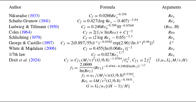
A substantial body of research has focused on developing predictive correlations based on local flow parameters, such as the Reynolds number (Nikuradse Reference Nikuradse1933; Schultz-Grunow Reference Schultz-Grunow1941; Ludwieg & Tillmann Reference Ludwieg and Tillmann1950; Coles Reference Coles1964; Schlichting Reference Schlichting1979; Fernholz & Finleyt Reference Fernholz and Finleyt1996; George & Castillo Reference George and Castillo1997; White & Majdalani Reference White and Majdalani2006; Nagib et al. Reference Nagib, Chauhan and Monkewitz2007) and the pressure-gradient parameter (Hutchins & Choi Reference Hutchins and Choi2002; Dixit & Ramesh Reference Dixit and Ramesh2009; Dixit et al. Reference Dixit, Gupta, Choudhary and Prabhakaran2024). Clauser (Reference Clauser1954) observed from experimental data that, for equilibrium APG-TBLs, the skin friction could be a double-valued function of the pressure gradient in a certain regime, a finding later supported by the theoretical analysis of Durbin & Belcher (Reference Durbin and Belcher1992). This inherent ambiguity highlights the limitations of purely local similarity models when applied to the complex, non-equilibrium physics of APG flows. Niegodajew, Dróżdż & Elsner (Reference Niegodajew, Dróżdż and Elsner2019) developed the corrected Clauser-chart method (Clauser Reference Clauser1956) for skin-friction estimation. The premise of this methodology is that, when properly scaled by
 $u_\tau$
, the intersection of the mean velocity profile with the logarithmic law (
 $\kappa =0.379$
and
 $C=3.56$
) coincides with the peak intensity of the large-scale motions, or the location of the maximum streamwise Reynolds stress. Crucially, this restriction dictates that the method is only valid for high Reynolds number (
 $\textit{Re}_\tau \gtrsim 1800$
) APG flows where a sufficient extent of the logarithmic region is guaranteed. Recent work by Dixit et al. (Reference Dixit, Gupta, Choudhary and Prabhakaran2024) linked skin friction directly to the structure and dynamics of the turbulent flow. They proposed a novel generalised scaling framework derived from the dynamical equations, which employs the total mean-flow kinetic energy
 $M=\int (u^2/\nu ) {\rm d}y$
and the shape factor function
 $G=U_{\!e}/u_\tau [(H-1)/H ]$
as surrogates for dynamical and boundary condition effects, respectively. This framework successfully unifies skin-friction prediction for an unprecedented range of flow types, including various APG-TBLs, without requiring resolution of the viscous sublayer or assumptions of a law-of-the-wall. Its demonstrated accuracy across standard and non-standard flows marks a considerable advance towards a universal prediction model grounded in turbulent transport physics. Furthermore, another class of skin-friction prediction methods based on normal integration of the velocity gradient and Reynolds stress (Fukagata, Iwamoto & Kasagi Reference Fukagata, Iwamoto and Kasagi2002; Mehdi & White Reference Mehdi and White2011; Renard & Deck Reference Renard and Deck2016; Li et al. Reference Li, Fan, Modesti and Cheng2019; Fan et al. Reference Fan, Atzori, Vinuesa, Gatti, Schlatter and Li2022) also warrants attention.
1.3. Outline
While the understanding of APG-TBL similarity has progressed significantly, particularly through mixed scaling theories that integrate both wall shear and pressure-gradient effects, most existing wall skin-friction prediction methods, especially those relying on inner scaling, are proven inadequate under the strong, non-equilibrium and history-dependent conditions inherent to APG flows (Sekimoto et al. Reference Sekimoto, Kitsios, Atkinson and Soria2019). The current study therefore attempts to develop a novel, physically consistent inner scaling defined by explicit functions of the wall shear stress, the imposed pressure gradient and the wall-normal distance, aiming to achieve two key objectives: first, to establish a universal scaling that yields self-similarity for the mean velocity profile across the entire boundary layer under diverse APG conditions, and, more significantly, to utilise this scaling formalism to construct a prediction model for skin friction (Nagib et al. Reference Nagib, Chauhan and Monkewitz2007). The central consideration is that, by accurately characterising the scaled flow structure, the wall skin-friction coefficient can be determined as an intrinsic part of the solution for a given pressure gradient and boundary-layer state, thereby moving beyond purely empirical correlations.
The rest of the paper is structured as follows. Section 2 provides a concise introduction to the derivation of the novel velocity scale and the associated wall skin-friction prediction model. The general validation of the new scaling framework is presented in § 3. In § 3.1, the datasets used in the present work are introduced briefly. Then, the efficacy of the novel velocity scale in collapsing mean velocity profiles subjected to diverse flow conditions is shown in § 3.2. Building upon the reconstructed self-similarity, an effective prediction model for wall skin friction is demonstrated in § 3.3, followed by a discussion from a momentum perspective in § 3.4. Finally, the main findings and conclusions are summarised in § 4.
2. Theoretical analysis
2.1. A comprehensive analysis of APG turbulent boundary layers
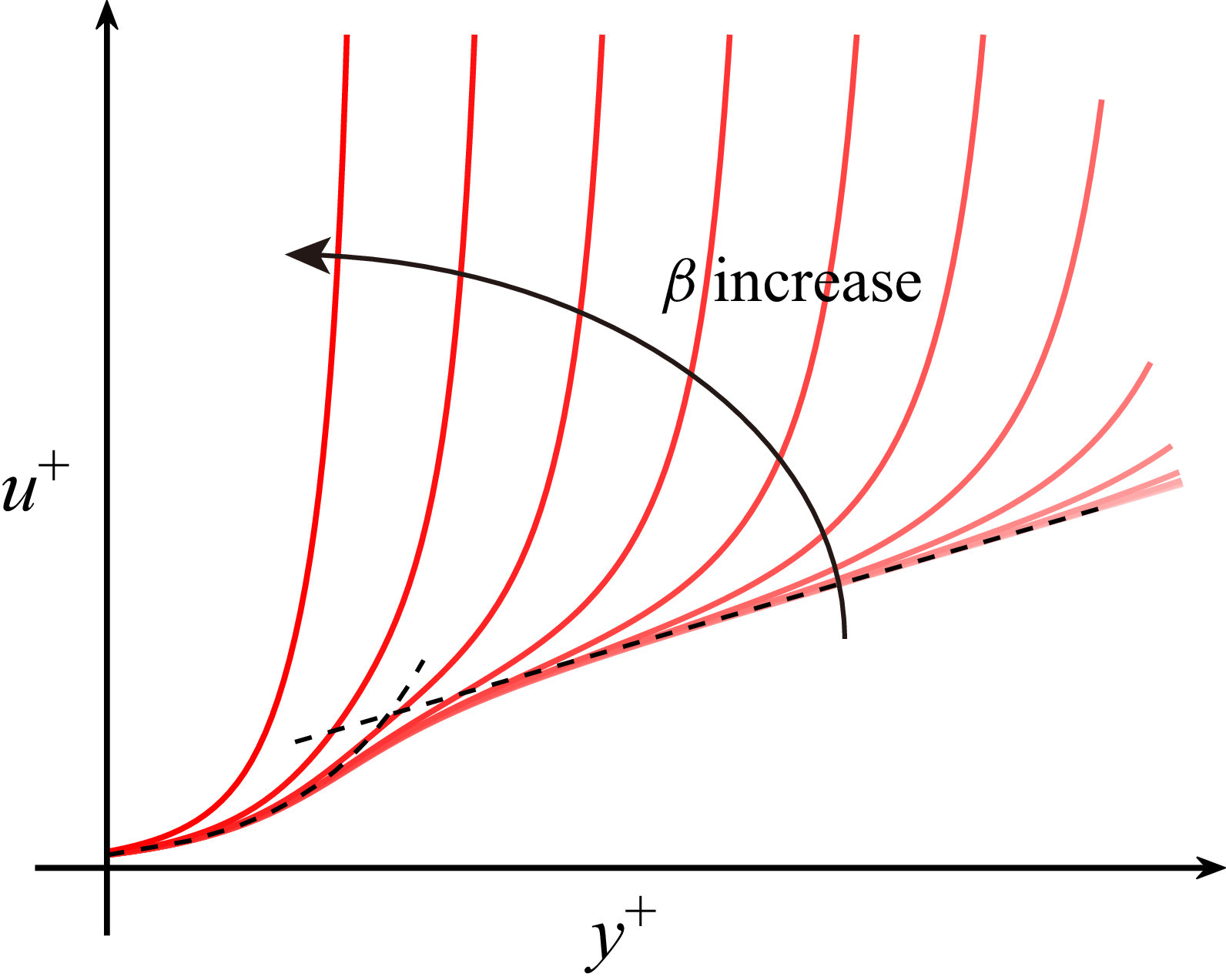
Figure 1 illustrates the fundamental structural modification of a TBL under the influence of an APG, where the mean velocity profiles are presented in the canonical inner scaling (
 $u^+$
versus
 $y^+$
). The dashed black line represents the standard viscous sublayer and logarithmic-law characteristic of a ZPG-TBL. The family of solid red lines depicts the mean velocity profiles as the pressure gradient increases, quantified by the Rotta–Clauser pressure-gradient parameter
 $\beta$
. With increasing
 $\beta$
, the inner-scaled profiles systematically depart from the standard log law, manifesting a significant wake-like defect in the outer layer. Further intensification of the pressure gradient drives a systemic distortion that affects the entire momentum balance of the boundary layer (Huang & Bradshaw Reference Huang and Bradshaw1995; Ahmed et al. Reference Ahmed, Zaman, Rezgui and Azarpeyvand2024). Critically, this structural change corresponds directly to a substantial reduction in the wall shear stress, as the profiles approach the characteristic shape observed immediately before separation. The complexity of this velocity profile evolution necessitates both a comprehensive understanding and a robust modelling effort.
Illustration of the inner-scaled velocity profile subjected to APG-TBL. The black dashed line represents the classical relationship for the viscous sublayer and the logarithmic region. The solid red line shows the change in the velocity profile as the APG gradually increases.

We assume that the APG-TBL is thin enough so that local wall curvature can be neglected at high Reynolds numbers, and that the flow has not yet separated and consider the two-dimensional Reynolds-averaged momentum equation for incompressible or weakly compressible turbulent flow, yielding (
 $x$
-component)
 \begin{equation} \begin{aligned} \underbrace {-\overline {\rho }\ \overline {u} \frac {\partial \overline u}{\partial x} - \overline {\rho }\frac {\partial \overline v}{\partial y}}_{\text{CD: convection diffusion}}+ \underbrace {-\frac {\partial \overline {p}}{\partial x}}_{\text{PG: pressure gradient}} +\\ \underbrace {\frac \partial {\partial x}\left (\overline {\tau }_{xx}\right ) + \frac \partial {\partial y} (\overline {\tau }_{xy})}_{\text{VD: viscous dissipation}} + \underbrace {\frac \partial {\partial x}\big (\!-\overline {\rho }\overline {u^{\prime }u^{\prime }}\big ) + \frac \partial {\partial y}\big (\!-\overline {\rho }\overline {u^{\prime }v^{\prime }}\big )}_{\text{TD: turbulent dissipation}}= 0,\\ \end{aligned} \end{equation}
where
 $\overline {\rho }$
is the density,
 $\overline {u}$
is the streamwise velocity,
 $\overline {v}$
is the normal velocity,
 $\overline {p}$
is the pressure,
 $\overline {\tau }_{xx}$
and
 $\overline {\tau }_{xy}$
are the viscous stresses and
 $\overline {u^{\prime }u^{\prime }}$
and
 $\overline {u^{\prime }v^{\prime }}$
are the Reynolds stresses, respectively. Following the Boussinesq hypothesis, the Reynolds shear stress is modelled as
 $-\overline {u^{\prime }v^{\prime }} = \overline {\mu }_t {\mathrm{d}\overline {u}}/{\mathrm{d}y}$
, where
 $\overline {\mu }_t$
is the turbulent (or eddy) viscosity coefficient. If we further ignore the convection terms and the streamwise derivative in the viscous terms (Durbin & Belcher Reference Durbin and Belcher1992; Shih et al. Reference Shih, Povinelli, Liu, Potapczuk and Lumley1999; Skote & Henningson Reference Skote and Henningson2002), we obtain the following simplified boundary-layer equation:
 \begin{equation} \begin{aligned} -\frac {\mathrm{d}\overline {p}}{\mathrm{d}x} + \frac {{d}}{\mathrm{d}y}\left [\left (\overline {\mu }+\overline {\mu _{t}}\right )\frac {\mathrm{d}\overline {u}}{\mathrm{d}y}\right ]& \simeq 0.\\ \end{aligned} \end{equation}
For brevity and in cases where no ambiguity is introduced, we omit the overline notation in the following part.
Considering the no-slip and no-penetration wall boundary conditions in the wall-normal direction, we approximate the wall-normal derivative of pressure as zero. This means that
 ${\mathrm{d}p}/{\mathrm{d}x}$
can be treated as a constant with respect to the wall-normal coordinate. By integrating (2.2) from the wall to a higher location, one can obtain the total stress as
 \begin{equation} \begin{aligned} \tau = (\mu +\mu _t) \frac {\mathrm{d}u}{\mathrm{d}y} &= \tau _w + \int _0^y \frac {\mathrm{d}p}{\mathrm{d}x} \mathrm{d}y \simeq \tau _w + \frac {\mathrm{d}p_{\!e}}{\mathrm{d}x} y = \tau _w (1+{K}y^+). \end{aligned} \end{equation}
The streamwise velocity can be obtained by integration from the wall surface to any height via
 \begin{equation} u = \int _0^y \frac {\tau _w + \frac {\mathrm{d}p_{\!e}}{\mathrm{d}x}y}{\mu (1+\mu _t/\mu )} \mathrm{d}y, \end{equation}
or in the viscous scale
 \begin{equation} u^+ = \int _0^{y^+} \frac {1+{K} y^+}{1+\mu _t/\mu } \mathrm{d}y^+. \end{equation}
In the viscous sublayer (or near-wall region) of the boundary layer, the turbulent viscosity coefficient is approximated as zero (
 $\mu _t/\mu \simeq 0$
). Hence, the velocity profile can be obtained through simple integration, yielding
 \begin{equation} u^+ = y^+ + \frac {1}{2}{K}(y^+)^2. \end{equation}
In the intermediate layer of the boundary layer (commonly referred to as the logarithmic region for ZPG-TBL), obtaining an accurate expression for the turbulent eddy viscosity coefficient is challenging. Classical ZPG boundary-layer theory usually employs a linear eddy viscosity model incorporating the Van Driest damping function (Van Driest Reference Van Driest1956), which leads to the relationship
 \begin{equation} \mu _t/\mu = \kappa y^+\big(1-e^{-y^+/A^+}\big)^2, \end{equation}
where
 $y^+=y\sqrt {\tau _w \rho }/\mu$
is the non-dimensional distance in inner scale, and
 $A^+=17$
is a constant. To adapt this relationship for applicability under APG conditions, we hypothesise that the wall shear stress within the equation can be replaced by the total stress, thereby resulting in the modified relation
 \begin{equation} \mu _t/\mu = \kappa \frac {y \sqrt {\tau \rho }}{\mu }\big (1-e^{-y\sqrt {\tau \rho }/(\mu A^+)} \big )^2 = \kappa y^+ \sqrt {1+{K}y^+} \big (1-e^{-y^+\sqrt {1+{K}y^+}/A^+} \big )^2. \end{equation}
Equation (2.5) can then be rewritten as
 \begin{equation} u^+ = \int _0^{y^+} \frac {1+{K} y^+}{1+\kappa y^+ \sqrt {1+{K} y^+} \big(1-e^{-y^+\sqrt {1+{K} y^+}/A^+} \big )^2} {\rm d}y^+. \end{equation}
If we choose the starting position (
 $y^+_l$
) of the integration such that
 $y_l^+\sqrt {1+{K} y_l^+} \gg A^+$
, we can then approximately derive
 \begin{equation} \begin{aligned} u^+ &\simeq \int _{y_l^+}^{y^+} \frac {1+{K} y^+}{1+\kappa y^+ \sqrt {1+{K} y^+}} \mathrm{d}y^+ + C(y_l^+, {K})\\ &\simeq \int _{y_l^+}^{y^+} \frac {\sqrt {1+{K} y^+}}{\kappa y^+} \mathrm{d}y^+ + C(y_l^+, {K})\\ &= \frac {1}{\kappa }\left ( \ln (y^+) - 2\ln \frac {\sqrt {1+{K} y^+}+1}{2}+2\Big(\sqrt {1+{K} y^+}-1\Big)\right ) + C(y_l^+, {K}), \end{aligned} \end{equation}
where
 $C(y_l^+, {K})$
accounts for the contribution of integration in the inner layer and is often considered as a constant. It is noteworthy that an expression similar to (2.10) was also derived by Townsend (Reference Townsend1961) based on the mixing-length hypothesis, and by Afzal (Reference Afzal1996) and Skote & Henningson (Reference Skote and Henningson2002) based on the effective matching of the inner-layer and outer-layer velocity gradients. If the pressure gradient diminishes, or
 $K=0$
, the classical log law can be readily recovered. An equivalent expression to (2.10), but in the first pressure-gradient velocity scale is
 \begin{equation} u^{\dagger } = \frac {1}{\kappa } \left (2\sqrt {\gamma ^2+y^{\dagger }}+\gamma \ln y^{\dagger }-2\gamma \ln \Big(\sqrt {\gamma ^2+y^{\dagger }}+\gamma \Big)\right ) + C, \end{equation}
where
 $\gamma =u_\tau /u_{\!p_1}$
represents the ratio of wall-friction velocity to the first pressure-gradient velocity, and
 $(u^{\dagger }=u/u_{\!p_1}, y^{\dagger }=yu_{\!p_1}/\nu )$
denotes the velocity and distance, non-dimensionalised by
 $u_{\!p_1}$
and
 $\nu$
. For flow at separation, the above equation reduces to the half-power law
 \begin{equation} u^{\dagger } = \frac {2}{\kappa } \sqrt {y^{\dagger }} + C, \end{equation}
consistent with the previous theory (Townsend Reference Townsend1961).
In the subsequent part, (2.10) will serve as the reference for the unified theoretical solution (with constants
 $\kappa =0.41$
and
 $C=5.2$
). Moreover, the
 $(u^+, y^+)$
relationship can be rescaled to other scales by employing the transformation
 \begin{equation} u^{\textit{inner}} = \left (\frac {u_{\tau }}{u_{\textit{inner}}}\right )u^+, \quad y^{\textit{inner}} = \left (\frac {u_{\textit{inner}}}{u_\tau }\right )y^+, \end{equation}
where
 $u_{\textit{inner}}$
can be
 $u_{{I}} = u_\tau + u_{\!p_1}$
(Shih et al. Reference Shih, Povinelli, Liu, Potapczuk and Lumley1999, Reference Shih, Povinelli, Liu and Chen2000),
 $u_{\text{II}} = \sqrt {u_\tau ^2 + (y/\delta ^*)u_{\!p_2}^2}$
(Sekimoto et al. Reference Sekimoto, Kitsios, Atkinson and Soria2019), and our newly developed velocity scale
 $u_{\circ }$
shown below.
2.2. A novel velocity scale developed for the APG boundary layer
As previously reported, velocity scaling with the friction velocity (
 $u_{\tau }$
) resulted in the contraction of the logarithmic layer and a significant upward shift of the wake region (Kitsios et al. Reference Kitsios, Sekimoto, Atkinson, Sillero, Borrell, Gungor, Jiménez and Soria2017), whilst scaling the velocity with the distance-dependent total stress velocity led to a considerable downshift of the intermediate-layer velocity (Sekimoto et al. Reference Sekimoto, Kitsios, Atkinson and Soria2019). This, in turn, poses a challenge in seeking the intrinsic self-similarity of APG-TBL. Based on physical considerations, we propose that a reasonable inner velocity scale should fulfil the following criteria:
-
(i) It should be a composite function of the wall-friction velocity (
 $u_{\tau }$
) and the pressure-gradient velocities (e.g.
$u_{\!p_1}, u_{\!p_2}$
).
-
(ii) It incorporates the influence of distance, particularly exhibiting a semi-power-law relationship,
$u \sim y^{1/2}$
, in the intermediate layer.


We begin by performing an order estimation. To facilitate the subsequent analysis, we define the boundary-layer thickness-based pressure-gradient parameter as
 \begin{equation} \beta _{\delta } = u_{\!p_3}^2/u_\tau ^2 = \frac {\delta }{\rho u_\tau ^2} \frac {\mathrm{d}p_{\!e}}{\mathrm{d}x}, \end{equation}
where
 $u_{\!p_3}=(\delta /\rho {\mathrm{d}p_{\!e}}/{\mathrm{d}x})^{1/2}$
is the redefined pressure-gradient velocity using the boundary-layer thickness instead of displacement thickness (Maciel et al. Reference Maciel, Wei, Gungor and Simens2018). Here, we emphasise that the redefined pressure-gradient velocity is related to the second pressure-gradient velocity through
 $u_{\!p_3} = u_{\!p_2}(\delta /\delta ^*)^{1/2}$
. Although the definition of
 $u_{\!p_3}$
is not strictly necessary, it will be beneficial for the subsequent representation of other physical quantities. For statistically steady APG-TBL flow, the external inviscid potential flow approximately satisfies the Bernoulli relation, i.e.
 \begin{equation} U_{\!e} \frac {\partial U_{\!e}}{\partial x} = - \frac {1}{\rho }\frac {\mathrm{d}p_{\!e}}{\mathrm{d}x}. \end{equation}
Assuming
 $x\sim L$
, where
 $L$
is the streamwise reference length, we obtain
 \begin{equation} \begin{aligned} u_{\!p_1}/U_{\!e} &\sim \left (\nu U_{\!e} \frac {\partial U_{\!e}}{\partial x}/U_{\!e}^3 \right )^{1/3} \sim \left (\frac {\nu /U_{\!e}}{\delta } \frac {{\delta }}{L}\right )^{1/3} \sim \textit{Re}_L^{-1/3} \sim \textit{Re}_{\delta }^{-1/3}({\delta }/L)^{1/3},\\ u_{\!p_3}/U_{\!e} &\sim \left ({\delta } U_{\!e} \frac {\partial U_{\!e}}{\partial x}/U_{\!e}^2 \right )^{1/2} \sim ({\delta }/L)^{1/2}.\\ \end{aligned} \end{equation}
The ratio of
 $u_{\!p_3}$
to
 $u_{\!p_1}$
is then derived as
 \begin{equation} u_{\!p_3}/u_{\!p_1} \sim ({\delta }/L)^{1/6} \textit{Re}_{\delta }^{1/3} \sim ({\delta }/L)^{1/2} \textit{Re}_L^{1/3}, \end{equation}
where
 $\textit{Re}_{\delta }=U_{\!e}\delta /\nu$
is the Reynolds number based on the edge thickness, and
 $\textit{Re}_{L}=U_{\!e} L/\nu$
is the Reynolds number associated with the streamwise length. Even under the most conservative assumption of a ZPG-TBL (Von Kármán Reference Von Kármán1934), where
 \begin{equation} \frac {\delta }{L} \sim \textit{Re}_L^{-1/5}, \end{equation}
it follows that
 \begin{equation} u_{\!p_3}/u_{\!p_1} \sim \textit{Re}_L^{7/30}. \end{equation}
Since the boundary layer under an APG is typically much thicker, the magnitude of
 $u_{\!p_3}$
is therefore considerably greater than that of
 $u_{\!p_1}$
.
On the other hand, the total stress along the wall-normal direction can be expressed as
 \begin{equation} \tau = \rho \left ( u_\tau ^2 + \frac {y}{\rho }\frac {\mathrm{d}p_{\!e}}{\mathrm{d}x} \right ) = \rho \left (u_\tau ^2 + y^{\dagger }(u_{\!p_1})^2 \right ) = \rho \left (u_\tau ^2 + ({y}/{\delta }) u_{\!p_3}^2 \right )\!. \end{equation}
Essentially,
 $u_{\!p_1}$
represents the pressure-gradient velocity scale at the inner layer of the boundary layer, whilst
 $u_{\!p_3}$
represents the pressure-gradient velocity scale in the outer layer. At the outer edge of the boundary layer, specifically at the position
 $y=\delta$
, one can derive
 \begin{equation} \frac {u_{\!p_3}}{u_{\!p_1}} = \sqrt {{(\delta )^{\dagger }}} = \sqrt {\frac {u_{\!p_1}}{u_\tau } \frac {u_\tau \delta }{\nu }} = K^{1/6} (\textit{Re}_\tau )^{1/2} = \beta _\delta ^{1/6} (\textit{Re}_\tau )^{1/3}. \end{equation}
This means that, for most APG-TBL flow (
 $\beta _\delta \gt \beta \gtrsim 1$
and
 $\textit{Re}_{\tau } \gg 1$
), we have
 $u_{\!p_3} \gg u_{\!p_1}$
, consistent with (2.19). Previously, De Graaff & Eaton (Reference De Graaff and Eaton2000) proposed a mixed velocity scale
 $\sqrt {U_{\!e} u_\tau }$
based on the wall-friction power. This scale successfully achieved better scaling of the Reynolds stress by incorporating both the friction velocity
 $u_{\tau }$
and the edge velocity
 $U_{\!e}$
, and can be rewritten as
 \begin{equation} \sqrt {U_{\!e} u_\tau } = u_\tau \sqrt {U_{\!e}/u_\tau } = u_\tau (U_{\!e}^+)^{1/2}. \end{equation}
Building on these insights, we introduce a new pressure-gradient velocity scale as
 \begin{equation} \sqrt {u_{\!p_1}u_{\!p_3}} = u_{\!p_1} \sqrt {u_{\!p_3}/u_{\!p_1}} = u_{\!p_1} \left (\sqrt {(\delta )^{\dagger }}\right )^{1/2}, \end{equation}
which incorporates both inner- and outer-layer effects. A comparison of (2.22) and (2.23) implicitly suggests that
 $U_{\!e} \sim \sqrt {\delta }$
, a finding that is consistent with the half-power law in the intermediate layer. By incorporating this mixed pressure-gradient velocity into the total stress balance equation,
 $\tau = \rho (u_\tau ^2 + ( {y}/{\rho })( {\mathrm{d}p}/{\mathrm{d}x}))$
, we finally propose a composite velocity scale for the mean velocity
 $u$
 \begin{equation} \begin{aligned} u_{\circ } &= \sqrt {(\rho ^+)\left [(u_\tau ^2 + ({y}/{\delta }) u_{\!p_1} u_{\!p_3}\right ]}\\ &= u_\tau \sqrt {(\rho ^+)\left [(1 + ({y}/{\delta }) K^{1/3} \beta _\delta ^{1/2}\right ]}=u_\tau \mathcal{F}_\circ , \end{aligned} \end{equation}
where
 $\rho ^+ = \rho /\rho _w$
represents the ratio of the local density to the density at the wall, and
 $\mathcal{F}_\circ =\sqrt {\rho ^+ [1+(y/\delta )u_{\!p_1}u_{\!p_3}/u_\tau ^2 ]}$
is the velocity transformation function that accounts for APG effects. Under the incompressible approximation, where
 $\rho ^+ = 1$
, this function simplifies to
 $\mathcal{F}_\circ =\sqrt {1+(y/\delta )u_{\!p_1}u_{\!p_3}/u_\tau ^2}$
. This scale is logically robust because it fundamentally fulfils the three required physical criteria:
-
(i) It automatically recovers the classical wall-friction velocity (
$u_{\tau }$
) when the pressure gradient approaches zero. -
(ii) It incorporates the wall-normal distance (
$y$
) and accounts for the half-power law under strong pressure gradients. -
(iii) It implicitly includes both inner- and outer-layer effects by blending
$u_{\!p_1}$
and
$u_{\!p_3}$
.


This composite scale thus represents a physically grounded attempt to achieve universal scaling in APG-TBL flows without significantly increasing mathematical complexity. It is noteworthy that the choice of the velocity scales
 $u_{\!p_1}$
and
 $u_{\!p_3}$
in (2.24), rather than the more commonly utilised
 $u_{\!p_2}$
, is motivated by the structural evolution of the boundary layer under strong APG. As demonstrated by Maciel et al. (Reference Maciel, Wei, Gungor and Simens2018),
 $u_{\!p_2}$
is tied to the displacement thickness
 $\delta ^*$
, an integral parameter that becomes less representative of the global outer-layer dynamics as the flow departs from equilibrium state. Specifically, the ratio
 $\delta ^*/\delta$
increases with
 $\beta$
, causing
 $\delta ^*$
to lose its scaling relevance for the intensified wake region. To address this, we utilise
 $u_{\!p_3}$
, which is related to
 $u_{\!p_2}$
via
 $u_{\!p_3} = u_{\!p_2} ( {\delta ^*}/{\delta } )^{-1/2}$
. This substitution effectively incorporates the full boundary-layer thickness
 $\delta$
, allowing the term
 $(y/\delta )u_{\!p_1}u_{\!p_3}$
to better represent the linear stress variation across the entire shear layer, which will be numerically validated later in Appendix A.
Alternatively, (2.24) can be rewritten as
 \begin{equation} \begin{aligned} u_{\circ } &= \sqrt {u_\tau ^2 + ({y}/{\delta ^*}) (\delta ^*/\delta )^{1/2} u_{\!p_1} u_{\!p_2}}\\ &= u_\tau \sqrt {1+({y}/{\delta ^*}) (\delta ^*/\delta )^{1/2} K^{1/3} \beta ^{1/2}} =u_\tau \mathcal{F}_\circ . \end{aligned} \end{equation}
The non-dimensional pressure-gradient parameters
 $K$
and
 $\beta$
represent the local flow characteristics, whereas the ratio
 $\delta ^*/\delta$
accounts for history-dependent effects (Bobke et al. Reference Bobke, Vinuesa, Örlü and Schlatter2017) arising from the accumulated influence of the streamwise pressure gradient.
2.3. Prediction of wall skin-friction coefficient
As previously mentioned, we have hypothesised that a carefully chosen mixed velocity scale can effectively collapse the mean boundary-layer profiles within an APG-TBL. Next, we further assume that, for high Reynolds number turbulent flow, the entire boundary layer can be represented by a logarithmic law when evaluating the wall skin-friction coefficient (Zhao & Fu Reference Zhao and Fu2025), expressed in a form analogous to the classic law of the wall
 \begin{equation} u^\circ = \frac {1}{\kappa }\ln y^\circ + C \iff y^\circ = e^{\kappa (u^\circ -C)}, \end{equation}
where
 $u^\circ = u/u_{\circ }$
is the velocity normalised by the present composite scale. The non-dimensional edge velocity
 $U_{\!e}^\circ$
based on this proposed scale becomes
 \begin{equation} U_{\!e}^\circ = U_{\!e}/(u_\tau \mathcal{F}_{\circ ,e}), \end{equation}
where
 $\mathcal{F}_{\circ ,e}$
is the value of
 $\mathcal{F}_{\circ }$
at the edge position.
Then, we can redefine the generalised displacement thickness and momentum thickness as
 \begin{equation} \lfloor \delta ^* \rfloor = \int _0^{\delta ^\circ } \frac {\rho }{\rho _e} \left(1-\frac {u^\circ }{U_{\!e}^\circ }\right) {d}(y^\circ \delta _v), \quad \lfloor \theta \rfloor = \int _0^{\delta ^\circ } \frac {\rho }{\rho _e} \frac {u^\circ }{U_{\!e}^\circ }\left(1-\frac {u^\circ }{U_{\!e}^\circ }\right) d(y^\circ \delta _v), \end{equation}
where
 $\delta _\nu =\mu _w / (\rho _w u_\tau )=\nu _w/u_\tau$
is the wall viscous scale.
For the above integral equations, the factor
 $\kappa U_{\!e}^\circ$
plays a dominant role, as we can deduce that
 \begin{equation} \begin{aligned} \kappa U_{\!e}^\circ = \ln (\delta ^\circ ) + \kappa C \gt \ln (\delta ^+) + \kappa C = \ln (\textit{Re}_\tau ) + \kappa C. \end{aligned} \end{equation}
Even at low friction Reynolds numbers, like
 $\textit{Re}_\tau =100$
, this magnitude remains substantial, as shown by the relationship
 $\kappa U_{\!e}^\circ \gt \ln (100)+0.41 \times 5.2=6.73 \gg 1$
. Utilising the Laplace integral method (or steepest descent for real integrals, see Appendix B), the above integrals can be evaluated by
 \begin{align} \begin{aligned} \lfloor \delta ^* \rfloor &= \int _0^{\delta ^\circ } \frac {\rho }{\rho _e} \left(1-\frac {u^\circ }{U_{\!e}^\circ }\right) {\kappa }e^{\kappa (u^\circ -C)}{d}(u^\circ \delta _v)\\ &=e^{-\kappa C}\delta _v \kappa U_{\!e}^\circ \int _0^1 \frac {\rho }{\rho _e}(1-Z) e^{\kappa Z U_{\!e}^\circ }\mathrm{d}Z \\ &\simeq \frac {1}{\kappa U_{\!e}^\circ }e^{\kappa (U_{\!e}^\circ -C)}\delta _v, \end{aligned} \end{align}
 \begin{align} \begin{aligned} \lfloor \theta \rfloor &= \int _0^{\delta ^\circ } \frac {\rho }{\rho _e} \frac {u^\circ }{U_{\!e}^\circ }\left(1-\frac {u^\circ }{U_{\!e}^\circ }\right) {\kappa }e^{\kappa (u^\circ -C)}d(u^\circ \delta _v)\\ &={\kappa }e^{-\kappa C}\delta _v U_{\!e}^\circ \int _0^1 \frac {\rho }{\rho _e}Z(1-Z) e^{\kappa Z U_{\!e}^\circ } {\rm d}Z\\ &\simeq \left (\frac {1}{\kappa U_{\!e}^\circ }-\frac {2}{(\kappa U_{\!e}^\circ )^2}\right )e^{\kappa (U_{\!e}^\circ -C)}\delta _v, \end{aligned} \end{align}
given that the dominant factor
 $\kappa U_{\!e}^\circ \gg 1$
. The shape factor is the ratio of the two integral thicknesses, given by
 \begin{equation} \mathcal{H} = \frac {\lfloor \delta ^* \rfloor }{\lfloor \theta \rfloor } \simeq \left (1-\frac {2}{\kappa U_{\!e}^\circ }\right )^{-1} \simeq 1 + \frac {2}{\kappa U_{\!e}^\circ }. \end{equation}
For high Reynolds number flows such that
 $U_{\!e}^\circ \to \infty$
, (2.31) implies that the redefined displacement thickness and momentum thickness are approximately equivalent.
Based on the above equations, the Reynolds numbers based on displacement thickness and momentum thickness can be represented by
 \begin{align} \begin{aligned} \textit{Re}_{\lfloor \delta ^* \rfloor } = \frac {\rho _e U_{\!e}}{\mu _e} \frac {1}{\kappa U_{\!e}^\circ }e^{\kappa (U_{\!e}^\circ -C)}\delta _v, \quad \textit{Re}_{\lfloor \theta \rfloor } = \frac {\rho _e U_{\!e}}{\mu _e} \left (\frac {1}{\kappa U_{\!e}^\circ }-\frac {2}{(\kappa U_{\!e}^\circ )^2}\right )e^{\kappa (U_{\!e}^\circ -C)}\delta _v. \end{aligned} \end{align}
From the definition of
 $\textit{Re}_{\lfloor \delta ^* \rfloor }$
and substituting
 $\delta _v = \mu _w / (\rho _w u_\tau )$
(the subscript
 $_w$
means the variable at the wall), one can obtain
 \begin{equation} \textit{Re}_{\lfloor \delta ^* \rfloor } = \frac {\rho _e U_{\!e}}{\mu _e} \boldsymbol{\cdot }\frac {1}{\kappa U_{\!e}^\circ }e^{\kappa (U_{\!e}^\circ -C)} \boldsymbol{\cdot }\frac {\mu _w}{\rho _w u_\tau }. \end{equation}
Rearranging to isolate the exponential term
 \begin{equation} e^{\kappa (U_{\!e}^\circ -C)} = \textit{Re}_{\lfloor \delta ^* \rfloor } \boldsymbol{\cdot }\frac {\mu _e}{\rho _e U_{\!e}} \boldsymbol{\cdot }\kappa U_{\!e}^\circ \boldsymbol{\cdot }\frac {\rho _w u_\tau }{\mu _w}. \end{equation}
Taking the natural logarithm of both sides and using the definition
 $U_{\!e}^\circ = U_{\!e}/(u_\tau \mathcal{F}_{\circ ,e})$
 \begin{equation} \kappa (U_{\!e}^\circ -C) = \ln \left [\textit{Re}_{\lfloor \delta ^* \rfloor } \boldsymbol{\cdot }\frac {\rho _w \mu _e}{\rho _e \mu _w} \boldsymbol{\cdot }\frac {\kappa U_{\!e}^\circ }{U_{\!e}^\circ \mathcal{F}_{\circ ,e}}\right ]\!. \end{equation}
Simplifying the term
 ${\rho _w \mu _e}/{\rho _e \mu _w}$
using the normalised viscosity
 $\mu _e^+ = \mu _e/\mu _w$
and density
 $\rho _e^+ = \rho _e/\rho _w$
 \begin{equation} \frac {\rho _w \mu _e}{\rho _e \mu _w} = \frac {\mu _e/\mu _w}{\rho _e/\rho _w} = \frac {\mu _e^+}{\rho _e^+}. \end{equation}
Thus, (2.33) becomes
 \begin{equation} \kappa (U_{\!e}^\circ -C) = \ln \left [\textit{Re}_{\lfloor \delta ^* \rfloor } \boldsymbol{\cdot }\frac {\mu _e^+}{\rho _e^+} \boldsymbol{\cdot }\frac {\kappa }{\mathcal{F}_{\circ ,e}}\right ]\!. \end{equation}
Dividing by
 $\kappa$
and rearranging terms yields the desired form for the displacement thickness-based wall skin-friction law
 \begin{equation} \sqrt {\frac {2}{C_{\!f}\rho _e^+\mathcal{F}_{\circ ,e}^{2}}} = \frac {1}{\kappa } \ln \left [\textit{Re}_{\lfloor \delta ^* \rfloor } \boldsymbol{\cdot }\frac {\mu _e^+}{\rho _e^+} \boldsymbol{\cdot }\mathcal{F}_{\circ ,e}^{-1}\right ] + \underbrace {\frac {1}{\kappa }\ln (\kappa ) + C}_{C_{\lfloor \delta ^* \rfloor }}. \end{equation}
Applying a similar derivation to the Reynolds number based on momentum thickness, we obtain
 \begin{equation} \sqrt {\frac {2}{C_{\!f}\rho _e^+\mathcal{F}_{\circ ,e}^{2}}} = \frac {1}{\kappa }\ln \left (\textit{Re}_{\lfloor \theta \rfloor } \frac {\mu _e^+}{\rho _e^+}\mathcal{F}_{\circ ,e}^{-1}\right ) + \underbrace {\frac {1}{\kappa } \ln (\mathcal{H} \kappa ) + C}_{C_{\lfloor \theta \rfloor }}. \end{equation}
The final equations are used to collapse APG data onto a ZPG formula, thereby successfully encapsulating the physical effects of weak compressibility (
 $\rho _e^+$
,
 $\mu _e^+$
) and the pressure gradient (
 $\mathcal{F}_{\circ ,e}$
) into two equivalent ZPG relations
 \begin{equation} \sqrt {\frac {2}{C_{\!f,0}}} = \frac {1}{\kappa } \ln (\textit{Re}_{\delta ^*,0}) + C_{ \lfloor \delta ^* \rfloor }, \quad C_{\!f,0} = \rho _e^+\mathcal{F}_{\circ ,e}^{2} C_{\!f}, \quad \textit{Re}_{\delta ^*,0} =\left (\frac {\mu _e^+}{\rho _e^+}\mathcal{F}_{\circ ,e}^{-1}\right ) \textit{Re}_{\lfloor \delta ^* \rfloor }, \end{equation}
 \begin{equation} \sqrt {\frac {2}{C_{\!f,0}}} = \frac {1}{\kappa } \ln (\textit{Re}_{\theta ,0}) + C_{\lfloor \theta \rfloor }, \quad C_{\!f,0} = \rho _e^+\mathcal{F}_{\circ ,e}^{2} C_{\!f}, \quad \textit{Re}_{\theta ,0} =\left ( \frac {\mu _e^+}{\rho _e^+} \mathcal{F}_{\circ ,e}^{-1}\right ) \textit{Re}_{\lfloor \theta \rfloor }. \end{equation}
If the weak compressibility is directly ignored, i.e.
 $\rho ^+=1$
and
 $\mu ^+=1$
, then (2.40) can be simplified as
 \begin{equation} \sqrt {\frac {2}{C_{\!f,0}}} = \frac {1}{\kappa } \ln (\textit{Re}_{\delta ^*,0}) + C_{ \lfloor \delta ^* \rfloor }, \quad C_{\!f,0} = \mathcal{F}_{\circ ,e}^{2} C_{\!f}, \quad \textit{Re}_{\delta ^*,0} =\left (\mathcal{F}_{\circ ,e}^{-1}\right ) \textit{Re}_{\lfloor \delta ^* \rfloor }, \end{equation}
 \begin{equation} \sqrt {\frac {2}{C_{\!f,0}}} = \frac {1}{\kappa } \ln (\textit{Re}_{\theta ,0}) + C_{\lfloor \theta \rfloor }, \quad C_{\!f,0} = \mathcal{F}_{\circ ,e}^{2} C_{\!f}, \quad \textit{Re}_{\theta ,0} =\left (\mathcal{F}_{\circ ,e}^{-1}\right ) \textit{Re}_{\lfloor \theta \rfloor }, \end{equation}
where the displacement thickness (
 $\lfloor \delta ^* \rfloor$
) or momentum thickness (
 $\lfloor \theta \rfloor$
) can be obtained by evaluating (2.28) or (2.30). It is worth noting that, although the shape factor approaches unity at high Reynolds numbers, it still exhibits a slow variation with the Reynolds number within a moderate range. Consequently, given that the coefficient
 $C_{\lfloor \theta \rfloor }$
incorporates the shape factor, its predictive capability for wall skin friction may be marginally less stable and effective than the method based on the displacement thickness Reynolds number.
A significant challenge in APG-TBL closure is the non-uniqueness of skin friction relative to integral parameters, as identified by Clauser (Reference Clauser1954) and Durbin & Belcher (Reference Durbin and Belcher1992). This double-valued ambiguity typically arises from the breakdown of local equilibrium, where outer-layer scales and upstream history prevent local pressure-gradient parameters from uniquely characterising the flow. The present model circumvents this issue through the composite velocity scale,
 $u_\circ = u_\tau \sqrt { 1+({y}/{\delta ^*}) (\delta ^*/\delta )^{1/2} K^{1/3} \beta ^{1/2}}$
. By explicitly retaining
 $u_\tau$
in conjunction with the pressure-gradient parameters (
 $K$
,
 $\beta$
) and the thickness ratio
 $\delta ^*/\delta$
, rather than collapsing the description into a single parameter, the model ensures a monotonic mapping between the velocity profile and the wall shear stress. Consequently, for any prescribed redefined displacement thickness
 $\lfloor \delta ^* \rfloor$
or momentum thickness
 $\lfloor \theta \rfloor$
, the model yields a unique and physically consistent value for
 $C_{\!f,0}$
. The physical friction coefficient is then recovered via
 $C_{\!f} = C_{\!f,0} \mathcal{F}_{\circ ,e}^{-2}$
.
3. Results and discussion
3.1. Description of the datasets
In this paper, we focus on incompressible or weakly compressible flows with APGs. To validate the proposed scaling law across a wide range of flow conditions, a comprehensive collection of established TBL datasets influenced by APGs was utilised. Figure 2 illustrates the distribution of these datasets in the parameter space defined by the friction Reynolds number (
 ${Re}_{\tau }$
) and the Rotta–Clauser pressure-gradient parameter (
 $\beta$
). The combined database spans a significant domain, with
 ${Re}_{\tau }$
ranging from approximately
 $10^2$
to
 $5\times 10^3$
and
 $\beta$
varying by more than two orders of magnitude, covering conditions from near ZPG (
 $\beta \simeq 10^{-1}$
) up to strong APG flows (
 $\beta \simeq 10^2$
). Specifically, the data incorporate numerical data from pressure-gradient flat plates (Bobke et al. Reference Bobke, Vinuesa, Örlü and Schlatter2016, Reference Bobke, Vinuesa, Örlü and Schlatter2017), curved plates (Mao et al. Reference Mao, Zhang, Hu, Wan, Sun and Zhang2026) and airfoils (Hosseini et al. Reference Hosseini, Vinuesa, Schlatter, Hanifi and Henningson2016; Vinuesa et al. Reference Vinuesa, Negi, Atzori, Hanifi, Henningson and Schlatter2018), as well as experimental measurements from ramps (Aubertine Reference Aubertine2005). This diverse set of external data is complemented by the inclusion of our own computed airfoil data (Hu et al. Reference Hu, Wan, Sun and Lu2026), ensuring a robust test platform that encompasses a variety of pressure gradients and surface geometries (see Appendix C).
Distribution range of friction Reynolds number and Rotta–Clauser pressure-gradient parameter for datasets from airfoils (Hosseini et al. Reference Hosseini, Vinuesa, Schlatter, Hanifi and Henningson2016; Vinuesa et al. Reference Vinuesa, Negi, Atzori, Hanifi, Henningson and Schlatter2018), pressure-gradient flat plates (Bobke et al. Reference Bobke, Vinuesa, Örlü and Schlatter2016, Reference Bobke, Vinuesa, Örlü and Schlatter2017), curved plates (Mao et al. Reference Mao, Zhang, Hu, Wan, Sun and Zhang2026), ramps (Aubertine Reference Aubertine2005) and the present computed airfoil data (Hu et al. Reference Hu, Wan, Sun and Lu2026).

3.2. A reconstructed self-similarity of velocity in inner scales
The fundamental goal of inner scaling is to achieve a universal velocity profile collapse across various flow conditions, a particularly challenging task in APG-TBL (Durbin & Belcher Reference Durbin and Belcher1992). For ease of comparison, we define the deviation as
 \begin{equation} \begin{aligned} \Delta u^{\textit{inner}}_{i, \textit{theory}} &= \mathrm{max}(|u_i^{\textit{inner}} - u_{{theory}}^{\textit{inner}}|),\\ \Delta u^{\textit{inner}}_{i, j} &= \mathrm{max}(|u_i^{\textit{inner}} - u_{j}^{\textit{inner}}|), \end{aligned} \end{equation}
where
 $u^{\textit{inner}}_i$
is a velocity profile expressed in inner scales, and
 $u^{\textit{inner}}_{{theory}}$
represents the theoretical prediction from (2.10) and (2.13). To elaborate,
 $\Delta u^{\textit{inner}}_{i, \textit{theory}}$
quantifies the deviation of the physical results from the theoretical law across various scalings, and
 $\Delta u^{\textit{inner}}_{i, j}$
demonstrates the inherent similarity (or collapse) among the different velocity profiles when scaled appropriately.
Comparison of the transformed velocity profiles under moderate pressure gradients (
 $\beta \lt 5$
): (a)
 $u^+$
with friction velocity, (b)
 $u^{\text{I}}$
with the first pressure-gradient velocity, (c)
 $u^{\text{II}}$
with the second pressure-gradient velocity and (d)
 $u^\circ$
with the present proposed velocity scale. (e) The maximum deviation from the theoretical prediction in different scales (
 $\Delta u_{i,{theory}}^{\textit{inner}}$
), and (f) the maximum deviation among different datasets in different scales (
 $\Delta u_{i,j}^{\textit{inner}}$
), or the similarity across various flow conditions.

Figure 3 presents a comparative analysis of the four scaling approaches (
 $u^+$
,
 $u^{\text{I}}$
,
 $u^{\text{II}}$
and
 $u^{\circ }$
) for moderate APG conditions (
 $\beta \lt 5$
). Figure 3(a) shows the classical viscous scaling (
 $u^+, y^+$
), where the scatter of the velocity profiles in the logarithmic region is evident, confirming the well-known failure of the classical friction velocity (
 $u_{\tau }$
) to collapse data under even mild pressure gradients (Galbraith, Sjolander & Head Reference Galbraith, Sjolander and Head1977; Huang & Bradshaw Reference Huang and Bradshaw1995; Bobke et al. Reference Bobke, Vinuesa, Örlü and Schlatter2017). The predecessor scales, (
 $u^{\text{I}}, y^{\text{I}}$
) (figure 3
b) and (
 $u^{\text{II}}, y^{\text{II}}$
) (figure 3
c), attempt to incorporate the pressure-gradient effect but still exhibit significant residual scatter, particularly near the outer edge of the log layer. Among the two, the (
 $u^{\text{I}}, y^{\text{I}}$
) scaling shows a relatively better performance in collapsing the profiles. However, the (
 $u^{\text{II}}, y^{\text{II}}$
) scaling introduces a perplexing and non-physical artefact (Sekimoto et al. Reference Sekimoto, Kitsios, Atkinson and Soria2019): the velocity profile becomes non-monotonic, peaking within the buffer layer (
 $y^{\text{II}}\simeq 30$
) or slightly higher positions before subsequently decreasing. This distortion clearly underscores the fundamental limitations and the non-physical nature of the (
 $u^{\text{II}}, y^{\text{II}}$
) velocity scale. In contrast, figure 3(d) demonstrates the superior performance of the present proposed velocity scale (
 $u^\circ$
) and corresponding wall-normal coordinate (
 $y^\circ$
). This scaling achieves a remarkably tight collapse of all velocity profiles across the viscous sublayer, buffer layer and the entirety of the logarithmic region. Crucially, the maximum deviation analysis presented in figure 3(e) highlights the quantitative shortcomings of these scales, where the deviation of
 $u^\circ$
from the theoretical prediction is substantially comparable to, or indeed lower than, that of all other tested scales within the crucial range of
 $y^{\textit{inner}} \lesssim 300$
. Furthermore, the flow self-similarity across different flow parameters warrants particular attention (Mellor & Gibson Reference Mellor and Gibson1966; Han et al. Reference Han, Ma and Yan2024). Figure 3(f) demonstrates that, in the region where
 $y^{\textit{inner}} \lt 60$
, the self-similarity achieved by the presently proposed velocity scale is comparable to that of the classical viscous scale. Moreover, in the region of
 $y^{\textit{inner}} \gtrsim 60$
, the proposed scale exhibits significantly stronger similarity compared with the other three scales at most locations, demonstrating its superior ability to collapse the mean velocity profiles in the intermediate layer.
Comparison of the transformed velocity profiles under strong pressure gradients (
 $\beta \geqslant 5$
): (a)
 $u^+$
with viscous scale, (b)
 $u^{\text{I}}$
with the first pressure-gradient velocity, (c)
 $u^{\text{II}}$
with the second pressure-gradient velocity and (d)
 $u^\circ$
with the present proposed velocity. (e) The maximum deviation from the theoretical prediction in different scales (
 $\Delta u_{i,{theory}}^{\textit{inner}}$
), and (f) the maximum deviation among different datasets in different scales (
 $\Delta u_{i,j}^{\textit{inner}}$
), or the similarity across various flow conditions.

The robustness and universality of the proposed scaling are also tested under strong APG conditions (
 $\beta \geqslant 5$
), which typically lead to extreme profile distortion and imminent separation, as presented in figure 4. Figure 4(a) confirms that the classical
 $u^+$
scale results in massive divergence across the logarithmic region, with velocity profiles
 $u^+$
spanning over 80 units at
 $y^+ \simeq 100$
. The
 $u^{\text{I}}$
scale, shown in figure 4(b), while marginally improving the fit in the range of
 $y^{\text{I}} \lesssim 40$
, still leaves unacceptable scatter at higher positions and fails to maintain the universal logarithmic slope. In figure 4(c), the introduction of the composite pressure-gradient velocity significantly reduces the magnitude of the inner-scale velocity, but the resultant non-physical velocity peak in the buffer layer retains its inherent drawback. Conversely, figure 4(d) illustrates the powerful capability of the present proposed velocity scale (
 $u^\circ$
). This scale successfully collapses the highly divergent strong APG velocity profiles onto the newly established law, at least in the range
 $y^\circ \lesssim 200$
. The corresponding deviation analysis, shown in figure 4(e), shows that the maximum deviation for
 $u^\circ$
remains significantly lower and more stable within
 $y^\circ \lesssim 200$
than any other scales tested. The ability of the (
 $u^\circ$
,
 $y^\circ$
) scaling to enforce the most improved self-similarity and collapse the velocity profiles even under conditions of imminent separation (figure 4
f), where the inner and outer flow layers are most severely decoupled, further demonstrates its superiority for complex APG-TBL. The success of the
 $u^\circ$
scaling under APG thus establishes an improved, universal framework for characterising velocity profiles across the entire TBL. Furthermore, Appendix D provides a detailed sensitivity analysis regarding boundary-layer thickness and flow compressibility. Complementing this, the self-similarity of Reynolds stress is examined in Appendix E.
3.3. Scaling law of
$C_{\!f}$
for turbulence subjected to APG

Comparison of the transformed wall skin-friction coefficient versus the Reynolds number: (a) original
 $C_{\!f}$
with displacement thickness Reynolds number, (b) transformed
 $C_{\!f1}$
with
 $\textit{Re}_1$
(Dixit et al. Reference Dixit, Gupta, Choudhary and Prabhakaran2024), (c) present transformed
 $C_{\!f,0}$
with displacement thickness Reynolds number
 $\textit{Re}_{\delta ^*,0}$
, (d) present transformed
 $C_{\!f,0}$
with momentum-thickness Reynolds number
 $\textit{Re}_{\theta ,0}$
, (e) relative prediction error with Dixit et al. (Reference Dixit, Gupta, Choudhary and Prabhakaran2024)’s model, with the
 $\pm 20\,\%$
error marked by the black dotted line, and (f) relative prediction error with the present model. In (c) and (d), the fitting relationships obtained under moderate APG are also displayed and serve as a consistent reference for all datasets.

The prediction of wall skin friction (
 $C_{\!f}$
) in TBLs under APG conditions represents one of the most critical and enduring unresolved challenges in computational and experimental fluid dynamics (Mellor & Gibson Reference Mellor and Gibson1966; Brown & Joubert Reference Brown and Joubert1969; Frei & Thomann Reference Frei and Thomann1980; Niegodajew et al. Reference Niegodajew, Dróżdż and Elsner2019). Figure 5 provides evidence of the enhanced predictive capability for
 $C_{\!f}$
inherent in the velocity self-similarity. Figure 5(a) clearly illustrates the well-known challenge: when data are plotted using conventional scaling, such as the skin-friction coefficient (
 $C_{\!f}$
) versus the displacement thickness Reynolds number (
 $\textit{Re}_{\delta ^*}$
), the results exhibit extreme scatter, confirming that traditional ZPG-based correlations (Nikuradse Reference Nikuradse1933; Schultz-Grunow Reference Schultz-Grunow1941; Ludwieg & Tillmann Reference Ludwieg and Tillmann1950; Coles Reference Coles1964; Schlichting Reference Schlichting1979; Fernholz & Finleyt Reference Fernholz and Finleyt1996; George & Castillo Reference George and Castillo1997; White & Majdalani Reference White and Majdalani2006; Nagib et al. Reference Nagib, Chauhan and Monkewitz2007) (see Appendix F) are rendered inadequate by strong pressure gradients. It is noteworthy that the model prediction by George & Castillo (Reference George and Castillo1997) yields comparatively better results by incorporating the friction Reynolds number (
 $\textit{Re}_\tau$
or
 $\delta ^+$
), but still loses predictive accuracy rapidly as the flow approaches separation. Figure 5(b) demonstrates the predictive capability of the Dixit et al. (Reference Dixit, Gupta, Choudhary and Prabhakaran2024) model, showing that the model indeed effectively reduces the scatter of the ‘skin-friction coefficient’ (
 $C_{\!f1}$
), but its predictive capability under strong APG exhibits certain limitations. Here,
 $C_{\!f1}$
and
 $\textit{Re}_1$
are defined by the following expressions:
 \begin{equation} \left \{ \begin{aligned} C_{\!f1} &= 2 f_1^2, \quad \textit{Re}_1 = \delta M/\nu ^2 (G/6.8)^{-0.5451} \\ f_1 &= \frac {u_\tau }{M/\nu } \left (\frac {G}{6.8}\right )^{0.5392}, \quad M = \int _0^\delta u^2 {\rm d}y, \quad G = U_{\!e}/u_\tau [(H-1)/H]. \end{aligned} \right . \end{equation}
Comparatively, figures 5(c) and 5(d) demonstrate the efficacy of the present proposed inner-scaled velocity transformation. When the transformed skin-friction coefficient (
 $C_{\!f,0}$
) is plotted against the redefined Reynolds numbers,
 $\textit{Re}_{\delta ^*,0}$
and
 $\textit{Re}_{\theta ,0}$
, respectively, the previously scattered data collapse into a remarkably tight and well-defined trend. This transformed relation suggests that, when properly characterised by
 $u_\circ$
, the TBL universally adheres to a consistent inner–outer scaling structure, irrespective of the pressure-gradient intensity (at least in the present datasets). This collapse is a major technical achievement, indicating that the new scaling parameter successfully unifies the underlying physics of both nearly ZPG and highly non-equilibrium APG flows. The quantitative superiority is confirmed in figures 5(e) and 5(f), where the relative error is defined by
 \begin{equation} \epsilon = \frac {C_{\!f,\textit{prediction}}-C_{\!f}}{C_{\!f}}\times 100\,\%. \end{equation}
While the prior model (Dixit et al. Reference Dixit, Gupta, Choudhary and Prabhakaran2024) exhibits relative prediction errors (
 $\epsilon _{\textit{Dixit}}$
) that demonstrate inadequate performance under strong APGs (figure 5
e), the present model maintains its prediction error (
 $\epsilon _{\circ }$
) within a tight band, generally constrained to be within
 $\pm 20\,\%$
across the entire measured range of
 $\textit{Re}_\tau$
and
 $\beta$
(figure 5
f). It is evident that for individual datasets, the error exhibits a complex dependency on the variations in the APG. Taking the airfoil dataset W2 as an example, the error initially manifests as a substantial negative bias before transitioning towards a positive deviation, potentially due to the history effects inherent in APG boundary layers. This trend is consistent with the evolution of the velocity profiles, where the rescaled velocity distribution closely aligns with the classical logarithmic law,
 $u^\circ =1/\kappa \ln (y^\circ )+C$
(see figure 3) under APG. As
 $\beta$
continues to increase, the velocity profile in the logarithmic region undergoes a downward shift (see figure 4), thereby resulting in an augmented negative bias. With a further increase in the APG, a pronounced elevation is observed in the velocity of the outer boundary layer, causing the error to trend towards a positive deviation. Furthermore, the
 $L_2$
norm of the relative prediction error, defined by
 \begin{equation} ||\epsilon || = \sqrt {\frac {1}{N}\sum _{i=1}^{N} \epsilon ^2}, \end{equation}
(
 $N$
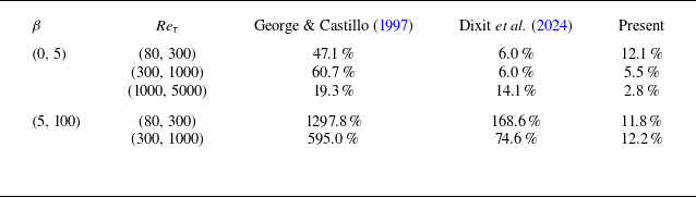
denotes the total number of samples within the specified parameter range) is listed in table 1. A comparative analysis across different parameter regimes highlights the limitations of prior scaling laws and the robustness of the current approach. While the George & Castillo (Reference George and Castillo1997) model exhibits significant discrepancies even at moderate pressure gradients, the Dixit et al. (Reference Dixit, Gupta, Choudhary and Prabhakaran2024) model shows improved performance primarily in the weak APG regime (
 $\beta \lt 5$
). However, both earlier models suffer a dramatic loss of fidelity for the current datasets as the flow enters the strong APG regime (
 $\beta \geqslant 5$
). In striking contrast, the present model maintains high predictive accuracy and physical consistency across the entire parameter space. It not only achieves a minimal error of
 $2.8\,\%$
at high Reynolds numbers in the weak APG range but also remains remarkably stable under high pressure gradients, keeping the
 $L_2$
error norm consistently near
 $12\,\%$
. This substantial enhancement in predictive accuracy, coupled with the successful attainment of robust data collapse, substantiates the underlying physical principles of the proposed inner scaling approach. These findings establish the current model as a robust and universally applicable methodology for predicting wall skin friction across various complex flow regimes.
Comparison of
 $L_2$
error norms for skin-friction predictions across the George & Castillo (Reference George and Castillo1997), Dixit et al. (Reference Dixit, Gupta, Choudhary and Prabhakaran2024) and the present models.

It is worth noting that approximating the entire boundary layer under an APG as a logarithmic distribution inevitably introduces specific errors. Specifically, this assumption tends to underestimate the contribution of velocity defect to displacement and momentum thicknesses within the viscous sublayer and buffer layer, while overemphasising the influence of the wake region on these integral parameters. While these discrepancies unavoidably affect the precision of the skin-friction prediction, the resulting errors remain well within acceptable limits, within approximately
 $\pm 20\,\%$
, for the parameter range investigated in the current study. Naturally, a more refined consideration of the velocity distributions within the inner and wake regions could further enhance predictive accuracy, although such an approach would necessarily increase the complexity of the modelling framework.
3.4. Discussion from a momentum perspective
The velocity scale
 $u_{\text{II}}$
is strictly derived from the simplified momentum balance in (2.2), which assumes a local equilibrium that often leads to severe deviations when exploring the self-similarity of the logarithmic region. To quantitatively assess this, we performed a comprehensive budget analysis of the mean momentum equation using direct numerical simulation (DNS) data from the W4 case (Hosseini et al. Reference Hosseini, Vinuesa, Schlatter, Hanifi and Henningson2016), as illustrated in figure 6. Across the range of Rotta–Clauser pressure-gradient parameters studied (
 $\beta = 1.0$
to
 $69.9$
), our analysis confirms that the pressure-gradient and viscous/turbulent diffusion terms are indeed the primary drivers of the momentum balance in the near-wall region (
 $y^{\textit{inner}} \lt 20$
). However, as one moves to higher wall-normal positions, the contribution from the convective diffusive (CD) term increases noticeably. This trend highlights the gradual breakdown of the thin-shear-layer simplification as history effects become more prominent in the outer part of the boundary layer. Our newly proposed velocity scale
 $u_\circ$
is specifically designed to address these limitations and represents a significant improvement over
 $u_{\text{II}}$
. Because
 $u_\circ$
consistently exhibits a lower magnitude than
 $u_{\text{II}}$
, it effectively denotes a discounted contribution from the pressure-gradient term. Physically, the present model recognises that the entire pressure gradient is not balanced solely by local stress; rather, a portion of pressure-gradient force is balanced by the convection term. In this sense,
 $u_\circ$
implicitly incorporates the influence of convection and history effects that (2.2) formally neglects. While it is difficult to precisely quantify the extent of this implicit representation across all flow conditions, we acknowledge that the inherent difficulty in capturing these non-local effects through a local scaling remains a likely factor in the predictive errors observed at the highest values of
 $\beta$
.
Budget analysis of the mean momentum equation: (a) original streamwise velocity field for the W4 case from Hosseini et al. (Reference Hosseini, Vinuesa, Schlatter, Hanifi and Henningson2016), (b) the Rotta–Clauser pressure-gradient parameter,
 $\beta$
, along the streamwise direction, where the red markers indicate the selected locations where
 $\beta = 1.0, 10.2$
and
 $69.9$
, (c) mean velocity profile at
 $\beta = 1.0$
scaled by both classical wall units and the present scaling, (d) momentum budget terms at
 $\beta = 1.0$
along the wall-normal direction, where PG is the pressure gradient, VD is the viscous dissipation, TD is the turbulent dissipation and CD is the convective diffusive term, and (e, f) and (g,h) are the corresponding velocity profiles and budget analyses for
 $\beta = 10.2$
and
 $\beta = 69.9$
, respectively.

4. Summary and conclusion
An APG fundamentally challenges turbulent flow modelling by drastically thickening the boundary layer, causing the shrinkage of the logarithmic layer, and disrupting self-similarity across the inner and outer layers. This non-equilibrium behaviour creates a flow with a strong tendency toward separation, making accurate turbulence modelling and skin-friction prediction the primary outstanding challenges. To address these deficiencies, this study introduces a novel velocity scale and proposes a related wall skin-friction prediction model. The main findings are summarised as follows.
Drawing inspiration from the linearly varied total stress along the normal direction, we proposed a new physically consistent inner scaling defined as
 $u_\circ =({u_{\tau }^2 + ({y}/{\delta } )u_{\!p_1}u_{\!p_3}})^{1/2}$
, which uniquely assimilates the friction velocity (
 $u_{\tau }$
), two distinct pressure-gradient velocity scales (
 $u_{\!p_1}$
and
 $u_{\!p_3}$
) and the
 $y^{1/2}$
dependency observed in the intermediate region. Based on a comprehensive examination of diverse APG datasets, spanning flow over flat plates, curved plates and airfoils across a wide parametric range (
 $10^2 \lesssim \textit{Re}_{\tau } \lesssim 5\times 10^3$
and
 $10^{-1} \lesssim \beta \lesssim 10^2$
), this proposed scale successfully recovers the classical logarithmic-law region across the entire range of investigated conditions. This crucial finding confirms the existence of a universal self-similarity under strong, non-equilibrium and history-dependent APG-TBLs. Building directly upon this consistently captured self-similarity, we formulated a novel wall skin-friction prediction methodology. The core hypothesis, that
 $C_{\!f}$
can be determined by correctly characterising the self-similarity APG-TBL flow, was quantitatively validated against high-fidelity numerical and experimental datasets ranging from ZPG to near-separation APG states. The resulting prediction strategy demonstrates excellent adaptability and improved accuracy across a wide distribution of relevant flow parameters.
In summary, this work contributes to both the deeper comprehension of APG-TBL structures and the practical prediction of wall skin friction. By advancing beyond purely empirical correlations and establishing a physically consistent prediction model, the identified self-similarity offers potential to enhance the fundamental understanding of pressure-gradient effects on wall skin friction, while also providing a potential framework for developing improved wall models for turbulence modelling in fundamentals and applications.
Acknowledgements
The authors express their gratitude to Professor R. Vinuesa (KTH Engineering Mechanics, Stockholm, Sweden) for kindly providing the numerical datasets, and to Professor T.-H. Shih for his valuable suggestions. The numerical computations were performed at Hefei Advanced Computing Centre.
Funding
This work was supported by the National Natural Science Foundation of China under Grant Nos. 12322210, 12402317 and 12388101. The first author also acknowledges financial support from the Fundamental Research Funds for the Central Universities (Grant No. WK2090000073) and the Science Foundation for Young Scientists of State Key Laboratory of High Temperature Gas Dynamics (Grant No. 2025QN06).
Declaration of interests
The authors report no conflicts of interest.
Appendix A. Comparison of the pressure-gradient velocity scale
$u_{\!p_2}$
and
$u_{\!p_3}$


Alternatively, composite velocity scales may be constructed using the following two formulations:
 \begin{equation} \begin{aligned} u_{\text{II}} &= \sqrt {u_\tau ^2+(y/\delta ^*)u_{\!p_2}^2} \to u_{\text{III}} = \sqrt {u_\tau ^2+(y/\delta ^*) u_{\!p_1}u_{\!p_2}},\\ u_{\text{II}} &= \sqrt {u_\tau ^2+(y/\delta )u_{\!p_3}^2} \to u_\circ = \sqrt {u_\tau ^2+(y/\delta ) u_{\!p_1}u_{\!p_3}}. \end{aligned} \end{equation}
To determine the most robust scaling formulation, the performance of the proposed scale,
 $u_\circ$
, is evaluated against the alternative scale,
 $u_{\text{III}}$
. As illustrated by the velocity profile collapses in figure 7, the
 $u_\circ$
-based formulation successfully accounts for the characteristic wake enhancement. In contrast, the
 $u_{\text{III}}$
formulation leads to significant scatter in the outer layer as
 $\beta$
increases, failing to maintain a universal profile. This discrepancy arises primarily because the
 $u_{\text{III}}$
formulation relies on local parameters and fails to account for the evolutionary history effects (see (2.25)) that become dominant in the outer region under strong pressure gradients.
Comparison of the velocity profile collapses using the classical wall viscous scale (
 $u_\tau$
) and the two composite velocity scales (
 $u_{\text{III}}$
,
 $u_\circ$
): (a–c) moderate pressure-gradient range (
 $\beta \lt 5$
), and (d–f) strong pressure-gradient range (
 $\beta \geqslant 5$
).

Appendix B. Integral analysis of the displacement and momentum thickness
Regardless of the coefficients
 $e^{-\kappa C}\delta _v \kappa U_{\!e}^\circ$
, the displacement thickness and momentum thickness in the present mixing velocity scale are defined by
 \begin{equation} \lfloor \delta ^* \rfloor (\alpha ) = \int _0^1 f(Z) (1-Z)e^{\alpha Z} \mathrm{d}Z, \quad \lfloor \theta \rfloor (\alpha ) = \int _0^1 f(Z) Z(1-Z)e^{\alpha Z} \mathrm{d}Z, \end{equation}
where
 $\alpha = \kappa U_{\!e}^\circ$
is a large number, and
 $f(Z)=\rho /\rho _e$
represents the slow variation of density along the normal direction. By considering the Laplace integral method, or the method of steepest descent for real integrals, the integral expression can be given by
 \begin{equation} \lfloor \delta ^* \rfloor (\alpha ) = e^{\alpha }\int _0^\infty f(1-t) t e^{-\alpha t} {\rm d}t, \quad \lfloor \theta \rfloor (\alpha ) = e^{\alpha }\int _0^\infty f(1-t) t (1-t)e^{-\alpha t} {\rm d}t. \end{equation}
The slowly changed function
 $f(1-t)$
is expanded in a Taylor series in
 \begin{equation} f(1-t) = f(1) - f^\prime (1)t + \frac {f^{\prime \prime }(1)}{2}t^2 + \ldots. \end{equation}
Finally, one can derive the displacement thickness as
 \begin{equation} \begin{aligned} \lfloor \delta ^* \rfloor &= e^{\alpha }\int _0^\infty \left [ f(1)t - f^{\prime }(1) t^2 + \frac {f^{\prime \prime }(1)}{2}t^3 + \ldots \right ] e^{-\alpha t}{\rm d}t\\ &= e^{\alpha } \left [ f(1)\frac {1}{\alpha ^2} - f^{\prime }(1)\frac {2}{\alpha ^3} + \frac {f^{\prime \prime }(1)}{2}\frac {6}{\alpha ^4}+\ldots \right ] = \frac {f(1)e^{\alpha }}{\alpha ^2} + O\left(\frac {f^\prime (1)}{\alpha ^3}\right)\!,\\ \end{aligned} \end{equation}
and similarly for the momentum thickness as
 \begin{equation} \begin{aligned} \lfloor \theta \rfloor &= e^{\alpha }\int _0^\infty \left [ f(1)t(1-t) - f^{\prime }(1) t^2(1-t) + \frac {f^{\prime \prime }(1)}{2}t^3(1-t) + \ldots \right ] e^{-\alpha t}{\rm d}t\\ &= e^{\alpha } \left \{ f(1)\left [\frac {1}{\alpha ^2}-\frac {2}{\alpha ^3}\right ] + f^{\prime }(1)\left [-\frac {2}{\alpha ^3}+\frac {6}{\alpha ^4}\right ] + \frac {f^{\prime \prime }(1)}{2}\left [\frac {6}{\alpha ^4}-\frac {24}{\alpha ^5}\right ]+\ldots \right \}\\ &=f(1)e^\alpha \left (\frac {1}{\alpha ^2}-\frac {2}{\alpha ^3} \right ) + O\left(\frac {f^\prime (1)}{\alpha ^3}\right)\!. \end{aligned} \end{equation}
Furthermore, the shape factor is defined by
 \begin{equation} \mathcal{H} = \frac {\lfloor \delta ^* \rfloor }{\lfloor \theta \rfloor } = \frac {1+o(1/\alpha )}{1-2/\alpha +o(1/\alpha )}=1+2/\alpha +o(1/\alpha ). \end{equation}
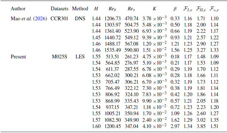
Parameters for pressure-gradient TBLs, derived from large eddy simulations (LESs) generated by Bobke et al. (Reference Bobke, Vinuesa, Örlü and Schlatter2016, Reference Bobke, Vinuesa, Örlü and Schlatter2017) using the SIMSON solver, and by Hosseini et al. (Reference Hosseini, Vinuesa, Schlatter, Hanifi and Henningson2016) and Vinuesa et al. (Reference Vinuesa, Negi, Atzori, Hanifi, Henningson and Schlatter2018) using the Nek5000 solver, as well as the experimental measurements by Aubertine (Reference Aubertine2005).

(Continued from table 2) Parameters for pressure-gradient TBLs, sourced from numerical simulations by Mao et al. (Reference Mao, Zhang, Hu, Wan, Sun and Zhang2026) using the PyFR solver, and from the present simulation results (Hu et al. Reference Hu, Wan, Sun and Lu2026) using the in-house Aero3DX solver.

Appendix C. Detailed parameters of the dataset
The detailed parameters of the datasets utilised in this work are presented in tables 2 and 3. The combined collection includes LESs by Bobke et al. (Reference Bobke, Vinuesa, Örlü and Schlatter2016, Reference Bobke, Vinuesa, Örlü and Schlatter2017), Hosseini et al. (Reference Hosseini, Vinuesa, Schlatter, Hanifi and Henningson2016) and Vinuesa et al. (Reference Vinuesa, Negi, Atzori, Hanifi, Henningson and Schlatter2018) spanning multiple orders of magnitude of the Rotta–Clauser parameter, high Reynolds number experiments by Aubertine (Reference Aubertine2005), DNSs of curved plate flows by Mao et al. (Reference Mao, Zhang, Hu, Wan, Sun and Zhang2026) and the present computational results for flow over a NACA-0012 airfoil at a
 $0^{\circ }$
angle of attack, Mach number
 $Ma=0.25$
and Reynolds number
 $\textit{Re}=4.08 \times 10^5$
(Hu et al. Reference Hu, Wan, Sun and Lu2026). In addition to the commonly referenced flow parameters, such as the shape factor
 $H$
, momentum-thickness Reynolds number
 $\textit{Re}_{\theta }$
, friction Reynolds number
 $\textit{Re}_{\tau }$
and pressure-gradient parameters
 $K$
and
 $\beta$
, we have additionally listed the values of three different velocity-scale factors at the boundary-layer edge:
 $\mathcal{F}_{{I},e}$
,
 $\mathcal{F}_{\textit{II},e}$
and
 $\mathcal{F}_{{\circ },e}$
. The magnitude of
 $\mathcal{F}_{\textit{II},e}$
is shown to be significantly higher than that of the other two velocity scales. Under milder pressure gradients, the distributions of
 $\mathcal{F}_{{\circ },e}$
and
 $\mathcal{F}_{{I},e}$
are more closely aligned. However, as the pressure gradient increases,
 $\mathcal{F}_{{\circ },e}$
exhibits larger numerical values, which correlates with its superior scaling capability under strong pressure gradients (see figures 3 and 4).
Appendix D. Sensitivity of the flow compressibility and the boundary-layer thickness
The current study primarily focuses on weakly compressible or incompressible flows, where the Mach number typically remains below
 $0.3$
. In such flow regimes, density variations are generally neglected. To quantitatively justify this simplification, a sensitivity analysis was performed on the M025S case, which features the highest Mach number among all cases investigated. Figure 8(a) illustrates the variation of the density ratio
 $\sqrt {\rho ^+} = \sqrt {\rho /\rho _w}$
along the wall-normal direction, revealing that the total variation remains below 1 %. Furthermore, figure 8(b) compares the inner-scaled velocity profiles
 $u^\circ$
both with and without the inclusion of density variations. The negligible discrepancy between these two profiles confirms that the incompressible approximation is robust and appropriate for the parameter range studied in this work.
Sensitivity analysis of compressibility effects for the airfoil case M025S (Hu et al. Reference Hu, Wan, Sun and Lu2026): (a) variation of the density ratio
 $\sqrt {\rho ^+} = \sqrt {\rho /\rho _w}$
along the wall-normal direction, (b) comparison of the inner-scaled velocity profiles with and without the inclusion of density variations.

Boundary-layer thickness
 $\delta$
is a pivotal physical parameter in the current velocity transformation, yet no universal consensus exists for its determination in flow under pressure gradients. To evaluate the sensitivity of our results to the definition of
 $\delta$
, we compared the diagnostic plotting method (Vinuesa et al. Reference Vinuesa, Bobke, Örlü and Schlatter2016) with the reconstructed inviscid velocity method (Griffin, Fu & Moin Reference Griffin, Fu and Moin2021), as illustrated in figure 9. Figure 9(a) reveals that boundary-layer thicknesses derived from the inviscid velocity method are systematically lower than those from the diagnostic method. While this discrepancy leads to slight variations in the rescaled velocity profiles shown in figure 9(b), the overall deviation remains relatively small. Furthermore, the skin-friction prediction performance and corresponding relative errors presented in figures 9(c) and 9(d) demonstrate that the prediction error shifts systematically towards the negative direction, yet remains contained within the
 $\pm 25\,\%$
range. We infer that although velocity similarity would likely persist with alternative definitions of
 $\delta$
, the constants associated with the logarithmic region, such as the slope and intercept, and the empirical coefficients in the skin-friction relationship might require recalibration for optimal fit across different boundary-layer thickness definitions. It is noteworthy that, apart from the boundary-layer thickness data provided by Aubertine (Reference Aubertine2005), which were directly measured by an experimental method, the boundary-layer thickness in all other datasets was obtained using a diagnostic plotting method.
Sensitivity analysis of the boundary-layer thickness
 $\delta$
for the airfoil case W4 (Vinuesa et al. Reference Vinuesa, Negi, Atzori, Hanifi, Henningson and Schlatter2018): (a) comparison of boundary-layer thicknesses determined via the diagnostic plotting method (Vinuesa et al. Reference Vinuesa, Bobke, Örlü and Schlatter2016) (circle markers) and the reconstructed inviscid velocity method (Griffin et al. Reference Griffin, Fu and Moin2021) (triangle markers), (b) velocity profiles in inner scales using the different definitions of
 $\delta$
, (c) comparison of the rescaled skin-friction coefficient
 $C_{\!f,0}$
against the momentum-thickness Reynolds number
 $\textit{Re}_{\delta ^*,0}$
and (d) relative error
 $\epsilon _{\textit{present}}$
across different methods as a function of the friction Reynolds number
 $\textit{Re}_\tau$
.

Appendix E. Self-similarity for Reynolds stress
In the present study, the primary objective of establishing self-similarity is the accurate prediction of wall skin friction. For this purpose, achieving a robust collapse of the mean velocity profiles across varying pressure gradients is sufficient to fulfil the fundamental modelling requirements. While the proposed composite scaling was initially intended to provide a unified normalisation for the Reynolds stresses as well, our comparative assessments, as demonstrated in figures 10 and 11, indicate that the conventional total stress scale,
 $u_{\text{II}}$
, remains superior for collapsing second-order statistics. This distinction is consistent with the physical realisation that the mechanisms governing mean momentum transport and those driving turbulent fluctuations do not necessarily scale identically under non-equilibrium conditions. Such an observation aligns with prior literature suggesting that the optimal scales for the mean velocity and Reynolds stresses are inherently distinct, particularly in the outer region where pressure-gradient effects are most pronounced (Sekimoto et al. Reference Sekimoto, Kitsios, Atkinson and Soria2019; Han et al. Reference Han, Ma and Yan2024). Consequently, we recommend a decoupled scaling approach: adopting the traditional stress-based scaling for investigations into inner-region turbulent structures, while utilising the present composite scale for mean-flow analysis and the determination of the skin-friction coefficient.
Comparison of the transformed shear stress
 $\overline {u^\prime v^\prime }$
under moderate pressure gradients (
 $\beta \lt 5$
): (a)
 $\overline {u^\prime v^\prime }$
scaled by
 $u_\tau$
, (b)
 $\overline {u^\prime v^\prime }$
scaled by
 $u_{{I}}$
, (c)
 $\overline {u^\prime v^\prime }$
scaled by
 $u_{\text{II}}$
and (d)
 $\overline {u^\prime v^\prime }$
scaled by the present proposed velocity scale
 $u_\circ$
.

Wall skin-friction predictive relations for both ZPG and APG flows.

Comparison of the transformed shear stress under strong pressure gradients (
 $\beta \geqslant 5$
): (a)
 $\overline {u^\prime v^\prime }$
scaled by
 $u_\tau$
, (b)
 $\overline {u^\prime v^\prime }$
scaled by
 $u_{{I}}$
, (c)
 $\overline {u^\prime v^\prime }$
scaled by
 $u_{\text{II}}$
and (d)
 $\overline {u^\prime v^\prime }$
scaled by the present proposed velocity scale
 $u_\circ$
.

Appendix F. Existing theoretical prediction formulas for wall skin friction
Table 4 shows the wall skin-friction prediction relations for ZPG and APG flows, with the empirical shape factor and streamwise Reynolds number provided by the following equations (Nagib et al. Reference Nagib, Chauhan and Monkewitz2007):
 \begin{equation} \begin{aligned} {H} &= 1/(1-7.135/U_{\!e}^+),\\ \textit{Re}_x &= (\textit{Re}_\theta /0.01277)^{1/0.8659}, \end{aligned} \end{equation}
where
 $U_{\!e}^+=1/0.384\ln (\textit{Re}_\theta )+4.127$
is the edge velocity, normalised by the viscous scale. A notable feature of the predictive model proposed by Dixit et al. (Reference Dixit, Gupta, Choudhary and Prabhakaran2024) is the introduction of an effective friction coefficient
 $C_{\!f1}$
, or effective friction factor
 $f_1$
, which is scaled using the velocity parameter
 $M/\nu$
and the boundary-layer thickness
 $\delta$
. To account for non-equilibrium history effects, the model incorporates Clauser’s shape factor,
 $G = (U_{\!e}/u_\tau )[(H-1)/H]$
(Clauser Reference Clauser1956), which provides a measure of the velocity profile’s deviation from equilibrium. In this framework,
 $M = \int _0^\delta U^2 {\rm d}y$
represents a critical integral quantity proportional to the total streamwise kinetic energy of the mean flow, thereby linking the local friction characteristics to the integral energy state of the boundary layer.