Introduction
Habitat loss and fragmentation are the main causes of biodiversity decline in agricultural landscapes (Liira et al. Reference Liira, Schmidt, Aavik, Arens, Augenstein, Bailey, Billeter, Bukáček, Burel, De Blust, De Cock, Dirksen, Edwards, Hamerský, Herzog, Klotz, Kühn, Le Coeur, Miklová, Roubalova, Schweiger, Smulders, Van Wingerden, Bugter and Zobel2008). Vertebrates with naturally small populations, strong habitat specialization and large body size are more sensitive to fragmentation (Ewers & Didham Reference Ewers and Didham2006, Henle et al. Reference Henle, Davies, Kleyer, Margules and Settele2004, Ribeiro et al. Reference Ribeiro, Colli, Caldwell, Ferreira, Batista and Soares2017). Habitat fragmentation acts as a filter on species with certain trait sets, leading to trait convergence and lower functional diversity (Grime Reference Grime2006).
Habitat connectivity has been quantified either through structural or functional connectivity (Tischendorf & Fahrig Reference Tischendorf and Fahrig2000). Structural connectivity can be estimated through landscape metrics in geographic information systems, or measuring distances between habitats or populations. Being easily quantified, structural connectivity is often misrepresented as functional connectivity, which describes a species’ intrinsic dispersal ability (Tischendorf & Fahrig Reference Tischendorf and Fahrig2000). Functional connectivity can be quantified by direct observation of species movements (e.g. radio-tracking), or indirectly through population genetic data or graph-theoretic approaches (Keller et al. Reference Keller, Brodbeck, Flöss, Vonwil and Holderegger2010), combining habitat and population attributes with the species’ dispersal abilities (Saura & Pascual-Hortal Reference Saura and Pascual-Hortal2007). Habitat patches or populations (nodes) are connected by links representing geographic distances (Saura & Pascual-Hortal Reference Saura and Pascual-Hortal2007, Saura & Torné Reference Saura and Torné2009), corridors or land uses. Nodes are considered connected if internode distance is inferior to the species’ maximum dispersal distance. This approach facilitates the determination of which features – nodes or links – influence the connectivity of habitat patches or populations in a landscape. Graph theory has been applied to landscape ecology (Risser et al. Reference Risser, Karr and Forman1984), but studies using these methods along with estimates of functional connectivity (e.g. gene flow, genetic diversity) remain scarce (Dyer et al. Reference Dyer, Chan, Gardiakos and Meadows2012, Neel Reference Neel2008).
We aim to determine which landscape features promote amphibian functional connectivity in an agricultural landscape located in the Araguaia river floodplain, Brazil. Amphibians have biphasic life cycles, highly permeable skin, ectothermic physiology and limited dispersal abilities, which increase their vulnerability to anthropogenic activities (Niemi & McDonald Reference Niemi and McDonald2004). We adapt the methods presented by Ribeiro et al. (Reference Ribeiro, Carretero, Sillero, Alarcos, Ortiz-Santaliestra, Lizana and Llorente2011), using species richness as surrogate for functional connectivity (Bailey et al. Reference Bailey, Schmidt-Entling, Eberhart, Herrmann, Hofer, Kormann and Herzog2010, Ribeiro et al. Reference Ribeiro, Carretero, Sillero, Alarcos, Ortiz-Santaliestra, Lizana and Llorente2011). Taxonomic, functional or phylogenetic diversity can thus be used as surrogates of functional connectivity, to understand how traits and lineages are filtered by fragmentation. Nodes with increased species or trait diversity may be more important for connectivity, due to landscape features improving accessibility or to increased microhabitat suitability. Hence, we considered both waterbody and landscape features potentially important for amphibians, to understand their role in determining waterbody importance for connectivity. We expect ponds surrounded by more forest patches, and providing more microhabitats for anurans will have increased importance for anuran connectivity in agricultural matrices. Our conclusions may help clarify how landscape configuration and composition act to shape anuran communities.
Methods
Study area and sampling design
Our study took place in the ecotone between the Brazilian Amazon rain forest and the cerrado savannas, in Lagoa da Confusão municipality, Tocantins state, central Brazil. The region is a seasonal floodplain between the rivers Formoso and Javaés, characterized by a tropical climate with a dry season, Aw in the Köppen climate classification (Alvares et al. Reference Alvares, Stape, Sentelhas, De Moraes Gonçalves and Sparovek2013). During the wet season, a flood pulse – up to 7 m in some places – inundates the region for 5 mo, being followed by a pronounced dry season (Irion et al. Reference Irion, Nunes, Nunes-Da-Cunha, De Arruda, Santos-Tambelini, Dias, Morais and Junk2016). The landscape consists of a mosaic of irrigated rice fields and natural habitats, primarily savannas and seasonally flooded grasslands interspersed with patches of alluvial forest – locally called ipucas – which remain flooded for longer periods than surrounding areas (Martins et al. Reference Martins, Brito, De Oliveira Filho, Da Silva and Silva2008, Valente et al. Reference Valente, Latrubesse and Ferreira2013). As these areas are unsuitable for cultivation, the agricultural landscapes in the study area are quite peculiar, with vast crops speckled with patches of native vegetation of variable dimensions.
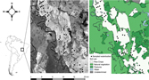
Irrigated rice fields in the study area present a dynamic hydrological regime, with variation between aquatic and terrestrial phases. When rice is being grown, from December to April, crop fields remain with surface water until harvest, when they are completely drained. After rice harvesting, crops may remain fallow or be replaced by other crops, such as soy or watermelon. Besides rice crops, the landscape is also occupied by pastures where cattle, emus and water buffalos roam. To ensure adequate representation of the spatial variability in this agricultural landscape, we sampled anurans in three to four lentic waterbodies from each of 10 rice fields along the Rio Formoso irrigation project, adding up to 35 waterbodies (Figure 1). Waterbodies were chosen based on type, area and hydroperiod; we chose small (25 m2) to large (1200 m2) temporary lentic waterbodies (Appendix 1).
Geographic location of the study area, an agricultural region dominated by irrigated rice crops, located in the Araguaia river floodplain, a savanna–rain forest ecotone in Tocantins, Brazil. Different soil uses are illustrated, and sampled waterbodies are represented by dark circles.

Anuran surveys
We conducted surveys during two rainy seasons, from February 2013 to April 2014. We sampled each waterbody 10 times in each rainy season, and visits to the same waterbody were at least 1 wk apart. Two trained observers performed nocturnal visual encounter surveys along a transect 10 m long by 1 m wide at the margin of each waterbody, for ~30 min. Every amphibian seen and captured was identified, measured, weighed, photographed and released near the site of capture. Given the homogeneity of microhabitats, weather and observers across sampled waterbodies, we assumed no significant variation occurred in species detection probabilities among sampling sites and occasions (Kéry et al. Reference Kéry, Royle and Schmid2005, Mazerolle et al. Reference Mazerolle, Bailey, Kendall, Andrew Royle, Converse and Nichols2007).
Waterbody features
We recorded the following variables along a 10 × 1-m transect on the margins of each sampled waterbody: bare ground, herbaceous vegetation, shaded ground, leaf litter, logs/rocks, aquatic vegetation, shrubs and trees, and herbaceous and shrub vegetation height and heterogeneity. At each metre along the transect, we placed a 50 × 50-cm gridded frame, subdivided into 25 10 × 10-cm squares, above the ground and recorded the proportion of squares with 50% or more coverage of each variable. At three randomly selected squares inside the gridded frame, we recorded the height of herbaceous vegetation. We measured or visually estimated (2–4 m, 4–10 m, <10 m) the height and heterogeneity (average number of species) of shrubs and trees in the transect and used the average height in analyses.
Landscape features
We used Google Earth satellite imagery of the year 2014 to record the following variables from each sampled waterbody, within buffers of 500-m, 1000-m and 1500-m radii: distance to closest waterbody, distance to closest forest patch, number of waterbodies, number of forest patches, total waterbody area, total forest area, mean forest patch area and mean waterbody area. Measurements were performed using Google Earth Pro v. 7.3.2.5495 tools. While compositional features, such as number of forest patches or total waterbody area, describe the proportion of different land uses around each waterbody, configurational features, such as distance to the closest forest patch or waterbody, specify the geometric arrangement of landscape features surrounding a waterbody. We quantified landscape features at three spatial scales (500-m, 1000-m and 1500-m buffers) to account for interspecific differences in the ability to disperse and endure in agricultural systems (Lemckert Reference Lemckert2004).
Trait data
We compiled life-history and ecological traits for each anuran species recorded in the study area: activity, habits, habitat, fossorial behaviour, adult snout-vent length (SVL), breeding site, breeding strategy, clutch size, parental care, breeding season, breeding pattern and geographic range size. We chose these traits based on perceived importance for determining species resilience to agricultural activities (Appendix 2) and on data availability. We compiled trait data from the literature, the AmphibiaWeb and IUCN online databases. If published data were unavailable, we relied on expert opinion or inferred trait information based on closely related species. Because breeding site, breeding season and breeding pattern were very homogeneous among the studied anurans (results not shown), we excluded these three traits from the following analyses.
Biodiversity metrics
For each waterbody, we calculated taxonomic diversity (TD), using Simpson’s diversity index, and functional diversity (FD) and phylogenetic diversity (PD) using Rao’s quadratic entropy (Botta-Dukát Reference Botta-Dukát2005). These metrics facilitate comparison among these three dimensions because Rao’s Q is an extended form of Simpson’s index that includes information on species dissimilarities. Rao’s Q corresponds to the sum of functional or phylogenetic distances between all species, weighted by the product of their relative abundances, and describes the abundance-weighted average difference among species from a community (Weiher Reference Weiher, Magurran and McGill2011). Functional and phylogenetic distances between species were obtained from pairwise dissimilarity matrices for all traits combined and for the phylogeny. Functional pairwise dissimilarity matrices were calculated using the Gower distance matrix, which quantifies dissimilarities with categorical and numerical attributes simultaneously (Botta-Dukát Reference Botta-Dukát2005). To promote meaningful comparisons among dimensions, we transformed each metric into its effective number of species, allowing direct interpretation of differences among indices (Jost Reference Jost2007). We calculated FD with function dfFD from package FD, and PD and TD with function raoD from package picante in program R 3.5.0.
Network connectivity
We used a graph theory approach to quantify the functional connectivity of the waterbody network, assessing the importance of each waterbody for the overall network connectivity with CONEFOR 2.6 (CS26, Saura & Pascual-Hortal Reference Saura and Pascual-Hortal2007, Saura & Torné Reference Saura and Torné2009). In this analysis, the network consists of nodes (waterbodies), within a matrix of inhospitable habitat (agriculture), interconnected by links representing species potential paths to disperse between two nodes. CS26 estimates functional connectivity, requiring as input the information necessary for describing both the structural (spatial arrangement of habitat patches, distances between nodes) and functional (dispersal abilities of the focal species, node attributes) aspects of connectivity (Saura & Torné Reference Saura and Torné2009). Hence, CS26 weights each node’s attributes, i.e. characteristics considered relevant for the analysis, such as habitat area, habitat quality, quality-weighted area or other appropriate attributes (e.g. species richness, population density, core area, carrying capacity, habitat suitability, etc.), along with distances between nodes, and the dispersal limits established for the focal species.
We used the Integral Index of Connectivity (IIC) to describe the overall connectivity of the waterbody network (Saura & Pascual-Hortal Reference Saura and Pascual-Hortal2007). IIC ranges between 0 and 1 and is defined as:
 $${\rm{IIC}} = {{\mathop \sum \nolimits_{{\rm{i}} = 1}^{\rm{n}} \mathop \sum \nolimits_{{\rm{j}} = 1}^{\rm{n}} {{{{\rm{a}}_{\rm{i}}}{{\rm{a}}_{\rm{j}}}} \over {1 + {\rm{n}}{{\rm{l}}_{{\rm{ij}}}}}}} \over {{\rm{A}}_{\rm{L}}^2}}$$
where n is the total number of nodes in the network, ai and aj are the attributes of nodes i and j, nlij is the number of links between nodes i and j, and AL is the total attribute of the network. To estimate the importance of each node (waterbody) for overall landscape connectivity, we used the delta value (dIIC):
 $${\rm{dIIC}}\left( {\rm{\% }} \right) = 100 \times {{{\rm{IIC}} - {\rm{IIC'}}} \over {{\rm{IIC}}}}$$
where IIC′ is the network connectivity after the removal of a given node from the landscape (Saura & Pascual-Hortal Reference Saura and Pascual-Hortal2007).
We used three diversity metrics (taxonomic (TD), functional (FD) and phylogenetic (PD) diversity) as node attributes, assuming that more reachable and suitable waterbodies will support more species, traits and lineages (Bailey et al. Reference Bailey, Schmidt-Entling, Eberhart, Herrmann, Hofer, Kormann and Herzog2010, Ribeiro et al. Reference Ribeiro, Carretero, Sillero, Alarcos, Ortiz-Santaliestra, Lizana and Llorente2011), and characterized links through the Euclidean distance between nodes. Studies on the dispersal ability of amphibians indicate that the maximum travelled distance from metamorphosis to adulthood is relatively variable among species (Kovar et al. Reference Kovar, Brabec, Vita and Bocek2009, Lemckert Reference Lemckert2004, Smith & Green Reference Smith and Green2005), commonly ranging from 10 to 2000 m. Therefore, we used four threshold dispersal distances (250, 500, 800 and 1000 m), which established two waterbodies as connected when they were closer than the threshold dispersal distance being considered (Saura & Pascual-Hortal Reference Saura and Pascual-Hortal2007, Saura & Torné Reference Saura and Torné2009). However, the degree of connection between each waterbody and the relative importance of each node for the connectivity of the whole network was approximated by CS26 according to each node’s attribute, i.e. TD, FD and PD. For each combination of diversity metric and threshold dispersal distance, we calculated IIC for the overall waterbody network and estimated dIIC for each waterbody. We then used correlation analysis to test at which threshold the relationship between dIIC and each anuran diversity metric is no longer significant, i.e. at what distance between waterbodies is anuran dispersal no longer translated by the diversity metrics used as proxies of anuran functional connectivity in the irrigated rice landscape.
Landscape predictors of connectivity
We used a principal component analysis of local waterbody characteristics to assess the contribution of each characteristic for overall variance and intercorrelation, using package FactoMineR (Lê et al. Reference Lê, Josse and Husson2008). The first two principal components (PCA1 and PCA2) – respectively representing 45% and 35% of the explained variance – were extracted (Appendix 3) and used as surrogates for original local waterbody feature predictors. In order to retain the nested structure of the landscape features while controlling collinearity between variables, each variable was transformed as a linear combination of the other variables (Rhodes et al. Reference Rhodes, McAlpine, Zuur, Smith, Ieno, Zuur, Ieno, Walker, Saveliev and Smith2009). Assuming X500, X1000, and X1500 are landscape variables measured at the 500-, 1000- and 1500-m landscape extents respectively, we generated a new set of variables Z500, Z1000, and Z1,500 such that: Z500 = X500, Z1000=X1000−X500, Z1500=X1500−X1000 (Rhodes et al. Reference Rhodes, McAlpine, Zuur, Smith, Ieno, Zuur, Ieno, Walker, Saveliev and Smith2009).
To examine the effects of waterbody and landscape features on waterbody importance for network connectivity (dIIC), we had to account for the nested structure of the explanatory landscape variables. Given that the spatial scale of nesting is associated with the spatial scale of auto-correlation, a reasonably straightforward way to deal with this problem is to use generalized linear mixed models (GLMMs) (Rhodes et al. Reference Rhodes, McAlpine, Zuur, Smith, Ieno, Zuur, Ieno, Walker, Saveliev and Smith2009), which takes into account the dependencies within sites. Hence, we implemented GLMMs using rice field as a random effect, because the 1000- and 1500-m buffers used to characterize the landscape features of each waterbody included other waterbodies within the same rice field. Random effects are especially useful for making inferences about a population when the data available are random samples of that population. Instead of anchoring results around heterogeneous intercepts, the data are used to estimate parameters of the distribution from which they were drawn. We fitted all GLMMs using package lme4.
We assessed the relative importance of predictor variables by fitting all possible combinations of the selected covariates using function dredge from the MuMIn package. For each covariate, we obtained the model averaged coefficient and importance value, calculated as the sum of Akaike weights over all models in which that particular covariate was included, using function model.avg of package MuMIn. We performed model averaging on the subset of models with ΔAIC < 2 (Burnham et al. Reference Burnham, Anderson, Anderson and Burnham2002). We conducted all statistical analyses in R 3.5.0.
Results
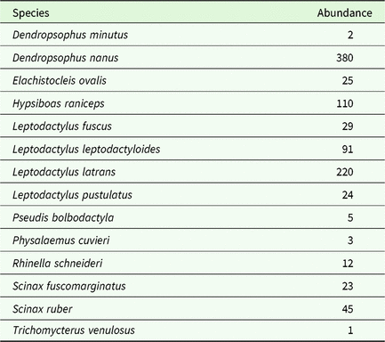
Overall, our sampling was effective in capturing the vast majority of the species present in rice fields (Appendix 4). The anuran community was composed of 14 species (Table 1), contrasting with 46 species recorded in the region’s pristine areas. Furthermore, there was a dominance of generalist hylids and leptodactylids (such as Dendropsophus nanus or L eptodactylus latrans, respectively) and low representation of specialist microhylids and bufonids. Over the whole waterbody network, mean ± SD was 0.388 ± 0.175 for TD, 0.959 ± 0.016 for FD and 0.172 ± 0.173 for PD.
Total abundance (number of individuals) of each anuran species recorded in 35 waterbodies embedded in rice fields, located in a savanna–rain forest ecotone (Brazil), and to which we applied graph-theoretic network analyses, to assess the importance of landscape features (forest patches, waterbodies) for anuran functional connectivity within the entire network. Specific nomenclature follows Frost et al. (Reference Frost, Grant, Faivovich, Bain, Haas, Haddad, De Sá, Channing, Wilkinson, Donnellan, Raxworthy, Campbell, Blotto, Moler, Drewes, Nussbaum, Lynch, Green and Wheeler2006)

The correlations between waterbody importance to overall network connectivity (dIIC) and anuran diversity metrics (TD, FD and PD) were conditional upon the threshold dispersal distance considered. TD was significantly correlated with waterbody importance for the 250-, 500- and 800-m thresholds (r250 = 0.81, P < 0.001; r500=0.79, P < 0.001; r800 = 0.64, P < 0.001) (Appendix 5). FD was significantly correlated with waterbody importance for the 250- and 500-m thresholds (r250 = 0.51, P = 0.002; r500 = 0.50, P = 0.002) (Appendix 5). PD was significantly correlated with waterbody importance for the 250-, 500- and 800-m thresholds (r250 = 0.66, P < 0.001; r500 = 0.66, P < 0.001; r800 = 0.55, P < 0.001) (Appendix 5). These results suggest that the functional connectivity between two waterbodies can be described by TD, FD or PD when amphibians are only able to disperse up to 800 m. However, they also indicate a lower ability of FD to represent functional connectivity; if local amphibians are able to disperse over 500 m, FD is no longer correlated with waterbody importance for connectivity.
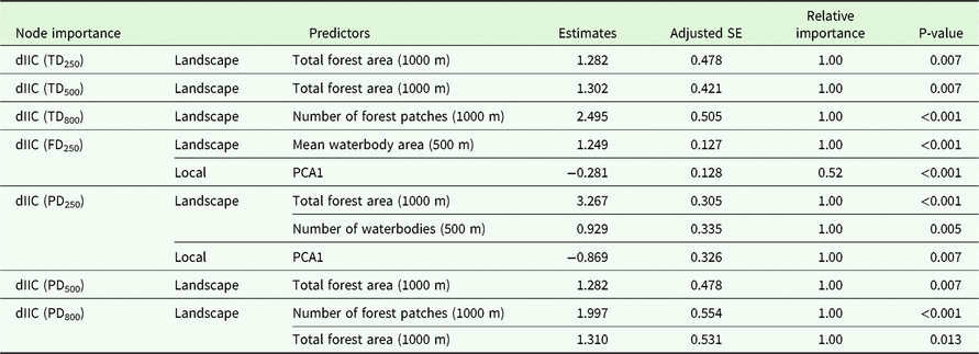
Local waterbody features significantly influenced waterbody importance to overall network connectivity (dIIC) (Table 2). Regarding FD and PD, waterbody importance decreased with increasing herbaceous heterogeneity (local variable highly correlated with PC1; Appendix 6).
Model averaged coefficient estimates of waterbody importance to overall network connectivity, calculated for 35 waterbodies embedded in rice fields, located in a savanna–rain forest ecotone (Brazil), and to which we applied graph-theoretic network analyses, to assess the importance of landscape features (forest patches, waterbodies) for anuran functional connectivity within the entire network. Adjusted standard errors, relative importance and P-value for node importance (dIIC) quantified using taxonomic (TD), functional (FD) or phylogenetic (PD) diversity as proxies for functional connectivity (intrinsic dispersal ability), and distance thresholds at which diversity metrics used were found to be significantly correlated with node importance (250, 500 and 800 m, depending on the metric). Node importance quantified with FD, assuming a dispersal limit of 500 m, could not be predicted by any of the variables used. Model averaging was performed on a subset of models with deltaAIC<2

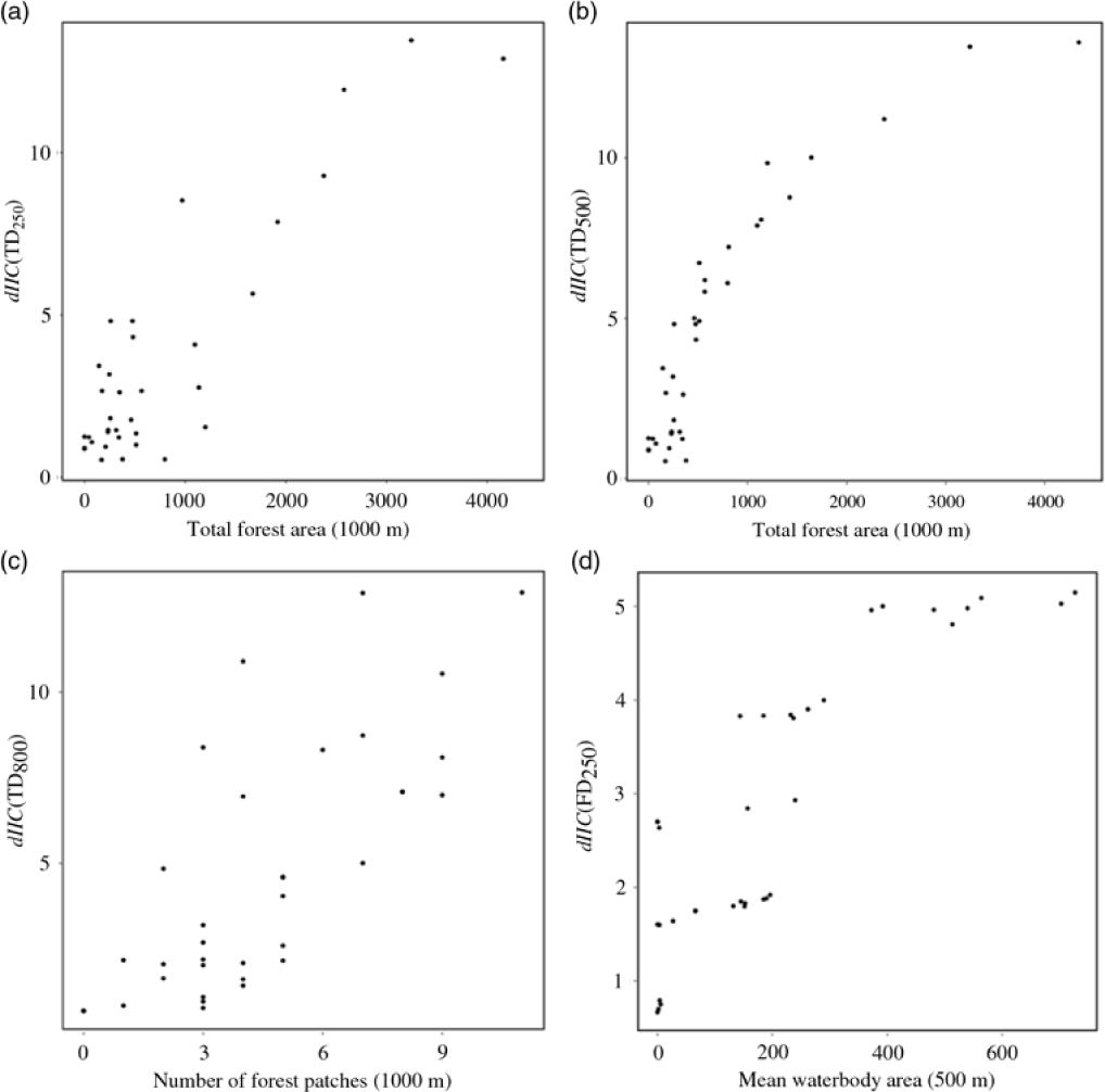
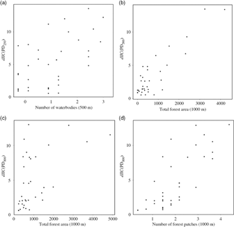
The most important landscape predictors of waterbody importance to overall network connectivity (dIIC) were: number of forest patches, total forest area, number and mean waterbody area in the vicinities of each waterbodies (Table 2). Regarding TD and PD, waterbody importance increased with increasing number of forest patches and total forest area (Figures 2a–c and 3). Regarding FD, waterbody importance increased with increasing mean waterbody area in the vicinity of waterbodies (Figure 2d).
Most significant predictors of node importance for connectivity using taxonomic (TD) and functional diversity (FD) as node attributes for functional connectivity, along with different distance thresholds for amphibian dispersal of 250, 500 and 800 m: variation of node importance for connectivity using TD as node attribute for functional connectivity for the 250-m distance threshold with total forest area (1000 m) (a); variation of node importance for connectivity using TD as node attribute for functional connectivity for the 500-m distance threshold with total forest area (1000 m) (b); variation of node importance for connectivity using TD as node attribute for functional connectivity for the 800-m distance threshold with number of forest patches (1000 m) (c); and variation of node importance for connectivity using FD as node attribute for functional connectivity for the 250-m distance threshold with mean waterbody area (500 m) (d).

Most significant model averaged predictors of node importance for connectivity using phylogenetic diversity (PD) as node attribute for functional connectivity, along with different distance thresholds for amphibian dispersal of 250, 500 and 800 m: variation of node importance for connectivity using PD as node attribute for functional connectivity for the 250-m distance threshold with number of waterbodies (500 m) (a); variation of node importance for connectivity using PD as node attribute for functional connectivity for the 500 m distance threshold with total forest area (1000 m) (b); variation of node importance for connectivity using PD as node attribute for functional connectivity for the 800 m distance threshold with total forest area (1000 m) (c); and variation of node importance for connectivity using PD as node attribute for functional connectivity for the 250 m distance threshold with number of forest patches (1000 m) (d).

Discussion
Anthropogenic habitat fragmentation is a major threat to native biodiversity worldwide (Fahrig Reference Fahrig2003), leading to increased stochastic extinction of local populations (Gonzalez et al. Reference Gonzalez, Lawton, Gilbert, Blackburn and Evans-Freke1998), decreased rescue effects (Gilbert-Norton et al. Reference Gilbert-Norton, Wilson, Stevens and Beard2010), reduced mutualistic interactions (Tewksbury et al. Reference Tewksbury, Levey, Haddad, Sargent, Orrock, Weldon, Danielson, Brinkerhoff, Damschen and Townsend2002, Van Geert et al. Reference Van Geert, Van Rossum and Triest2010) and decreased genetic diversity of populations (Cascante et al. Reference Cascante, Quesada, Lobo and Fuchs2002). The enhancement of habitat connectivity has been repeatedly recommended to mitigate the negative effects of fragmentation (Bennett Reference Bennett1990, Noss Reference Noss2003), especially in highly biodiverse and anthropogenic landscapes.
We found a significant positive relationship between anuran diversity metrics and waterbody importance for connectivity, if local amphibians are overall assumed to have a distance threshold inferior to 800 m. The amphibian community found in rice crops is a subset of the region’s native community dominated by generalist species, with small body size (Ribeiro et al. Reference Ribeiro, Colli, Caldwell, Ferreira, Batista and Soares2017). Given the association between dispersal ability and large body size, due to an ability to better control both heat and water balance (Olalla-Tárraga et al. Reference Olalla-Tárraga, McInnes, Bini, Diniz-Filho, Fritz, Hawkins, Hortal, Orme, Rahbek, Rodríguez and Purvis2011, Sodhi et al. Reference Sodhi, Bickford, Diesmos, Lee, Koh, Brook, Sekercioglu and Bradshaw2008), and the low body condition found in this community (Ribeiro et al. Reference Ribeiro, Colli, Caldwell, Ferreira, Batista and Soares2017), we can safely assume that high dispersal ability of small amphibians within this agricultural matrix is unlikely. Rice crops can be extremely hostile for anurans due to decreased protection from predation, increased exposure to extreme temperatures and low humidity, agrochemicals and heavy machinery associated with crop management through all life stages.
Adopting TD, FD and PD as proxies for functional connectivity is substantiated by the premise that more accessible sites will host more species, traits and lineages, considering habitat suitability is similar, as all waterbodies are embedded in the same agricultural matrix. The relationship between landscape connectivity and anuran diversity metrics is unambiguous, indicating that the accumulation of amphibian species, traits and lineages in breeding ponds is, even if partially, related to the spatial position of the pond in relation to the other ponds nearby. Our results corroborate those found by Cunningham et al. (Reference Cunningham, Calhoun and Glanz2007) and Ribeiro et al. (Reference Ribeiro, Carretero, Sillero, Alarcos, Ortiz-Santaliestra, Lizana and Llorente2011). In fact, according to Cunningham et al. (Reference Cunningham, Calhoun and Glanz2007), wetland connectivity is the best variable at distinguishing wetlands with high amphibian species richness from those with low species richness. Although species richness is a fundamental measurement of regional diversity and extremely useful in conservation planning, it could be misleading, as accounting only for species number leaves important community and ecosystem-level parameters unassessed. For example, in this study the maximum distance threshold at which diversity and functional connectivity were correlated was 500 m regarding trait diversity and 800 m regarding taxonomic and phylogenic diversity. This means that if amphibians are able to disperse over 500 m, waterbody FD is no longer a reliable proxy of its importance for connectivity. Variation was low for FD, and higher for TD and PD over the whole network, indicating trait attributes found in this community are few and convergent. Fragmentation appears to have acted as a very fine filter on the trait set originally found in this region’s anuran community, ensuring that only the very few traits that enable anurans to endure in this environment have persisted. Consequently, FD differences are more easily dissolved over the whole network, making it an unreliable proxy for functional connectivity, or waterbody importance for connectivity beyond that 500 m threshold. Nonetheless, our results suggest TD and PD can be used as reliable proxies to functional connectivity if amphibians are able disperse to a maximum of 800 m. This enforces the importance of taking multiple metrics and scales to approach the effects of human activities on biodiversity.
Pond breeding amphibians typically exist in local populations associated with discrete breeding pools. With low dispersal ability and the potential for asynchronous dynamics among local populations, meta-population dynamics may play an important role in long-term population persistence (Gamble et al. Reference Gamble, McGarigal and Compton2007, Semlitsch Reference Semlitsch2002, Smith & Green Reference Smith and Green2005), especially in unstable anthropogenic landscapes. Hence, conservation efforts limited to the protection of individual pools may be ineffective over the long term if connectivity among pools is not maintained (Gibbs Reference Gibbs1993, Gibbs & Shriver Reference Gibbs and Shriver2005). Maintenance and enhancement of spatial connectivity among fragmented natural and semi-natural habitats is one of the main challenges for ecological management and conservation biology. However, although the structural properties of landscapes are widely used as indicators of biodiversity in practical landscape planning, they may not have a straightforward effect on functional connectivity, i.e. the way each species responds to landscape structure (Tischendorf & Fahrig Reference Tischendorf and Fahrig2000).
Given that diversity metrics also represent habitat suitability, as more species will breed successfully in more suitable waterbodies, functional connectivity may be overestimated if those factors related to habitat quality are not accounted for. Functional connectivity can only be affected by species’ intrinsic dispersal abilities or by landscape features. We regressed several local and landscape variables on node importance estimates derived from graph-theory analyses to assess which features are more determinant for increasing waterbody importance for connectivity in an agricultural landscape. We found that total forest patch area and abundance within 1000 m from a waterbody, as well as waterbody abundance and area within 500 m from a waterbody were the most important predictors of node importance for connectivity. The importance of forest fragments for dispersal in anthropogenic landscapes has been identified before. Janin et al. (Reference Janin, Léna, Ray, Delacourt, Allemand and Joly2009) found that the landscape matrix strongly influenced toad occurrence, with forests and meadows causing low resistance to toad movement, and crops posing intermediate to high resistance to toad movement. Popescu & Hunter (Reference Popescu and Hunter2011) found clear-cuts to be significant barriers to amphibian dispersal, altering the movements of emigrating juveniles from waterbodies. The low permeability of clear-cuts and other open-canopy habitats to juvenile amphibian movement has been previously recorded (Rothermel Reference Rothermel2004, Rothermel & Semlitsch Reference Rothermel and Semlitsch2002). Boissinot et al. (Reference Boissinot, Grillet, Besnard and Lourdais2015) also concluded that the proportion of forest surface area was a critical determinant of frog presence and abundance.
Our results also suggest that node importance defined by functional and phylogenetic diversity is promoted by both waterbody abundance and area in the vicinities of each waterbody (500 m). Marsh et al. (Reference Marsh, Fegraus and Harrison1999) established breeding pond isolation as a primary determinant of the temporal and spatial dynamics of pond use by the Túngara frog, as egg masses in ponds decreased with pond isolation, independently of habitat quality. Despite pertaining to frog populations in pristine sites, these results indicate that pond networks may be even more important for maintaining amphibian populations in agricultural landscapes.
Our findings indicate that to maximize amphibian dispersal in rice crops, we must ensure abundant and large forest patches in the vicinities of waterbodies, as well as a network of abundant waterbodies. Amphibian dispersal is highly important for the maintenance of amphibian populations, and substantially compromised in anthropogenic landscapes, such as crops. In Brazil, the laxness of the current environmental legislation poses a massive challenge to an already difficult endeavour of implementing management and conservation actions targeting native faunal communities. Increased knowledge can therefore contribute to amphibian conservation, improving the effectiveness of management actions. Current protection of Brazilian biomes is deficient and, without highly guided and informed actions, native amphibian communities may be critically compromised.
Author ORCIDs
Joana Ribeiro https://orcid.org/0000-0002-3755-5785
Acknowledgements
We would like to thank the Editor and two anonymous reviewers, whose suggestions contributed to improving this paper.
Financial support
Joana Ribeiro thanks FCT (Foundation for Science and Technology) for a PhD fellowship (reference SFRH / BD / 51414 / 2011). Guarino R. Colli thanks Coordenação de Apoio à Formação de Pessoal de Nível Superior – CAPES, Conselho Nacional do Desenvolvimento Científico e Tecnológico – CNPq, Fundação de Apoio à Pesquisa do Distrito Federal – FAPDF, and the Partnerships for Enhanced Engagement in Research (PEER) program for financial support.
Appendix 1
Local waterbody characteristics of all 35 waterbodies embedded in 10 rice fields in a savanna-rain forest ecotone to which we applied graph-theoretic network analyses, to assess the importance of landscape features (forest patches, waterbodies) for anuran functional connectivity within the entire network. These variables were subjected to principal component analysis, from which three principal components were extracted and used in GLMM to analyse the importance of local waterbody characteristic for anuran diversity metrics. Herbaceous and shrub vegetation heterogeneity correspond to the average number of different species present at each metre walked in the 10 × 1-m transect (Schulz et al. Reference Schulz, Bechtold and Zarnoch2009).

Appendix 2
Anuran traits considered for calculating functional diversity for each of the 35 sampled waterbodies embedded in rice fields, located in a savanna-rain forest ecotone (Brazil) and to which we applied graph-theoretic network analyses, to assess the importance of landscape features (forest patches, waterbodies) for anuran functional connectivity within the entire network. Trait attributes, definition and relevance for each species trait used on this study are stated.

Appendix 3
Contribution of each variable for the first two principal components extracted from the PCA performed on local characteristics of the 35 sampled waterbodies embedded in rice fields, located in a savanna-rain forest ecotone (Brazil) and to which we applied graph-theoretic network analyses, to assess the importance of landscape features (forest patches, waterbodies) for anuran functional connectivity within the entire network.

Appendix 4
Species accumulation curve for the amphibian community found in the 35 sampled waterbodies embedded in rice fields, located in a savanna–rain forest ecotone (Brazil), and to which we applied graph-theoretic network analyses to assess the importance of landscape features (forest patches, waterbodies) for anuran functional connectivity within the entire network. Representation of Chao1 estimates for increased species number recorded if sampling sites were increased to 50; standard errors represented as dotted lines.

Appendix 5
Correlation between TD, FD and PD used as proxies for functional connectivity and node importance for overall connectivity calculated for 35 sampled waterbodies embedded in rice fields, located in a savanna–rain forest ecotone (Brazil), and to which we applied graph-theoretic network analyses, to assess the importance of landscape features (forest patches, waterbodies) for anuran functional connectivity within the entire network. Node importance for overall connectivity was calculated with CS26, considering distance thresholds considered meaningful (250, 500, 800 m).

Appendix 6
Variation of waterbody importance for connectivity using FD250 (a) and PD250 (b) as node attributes for functional connectivity, along with herbaceous heterogeneity (local variable more closely associated with principal component 1 (PCA1)), considering 35 sampled waterbodies embedded in rice fields, located in a savanna–rain forest ecotone (Brazil), and to which we applied graph-theoretic network analyses, to assess the importance of landscape features (forest patches, waterbodies) for anuran functional connectivity within the entire network.