4.1. Single-parameter

We consider a classical two-dimensional open flow around a circular cylinder, with the relevant equations as

(4.1) \begin{align}& \frac {\partial \boldsymbol{U}}{\partial \tau }+\boldsymbol{U}\cdot \nabla \boldsymbol{U}=-\nabla P+{\textit{Re}}^{-1}\nabla ^2\boldsymbol{U}, \end{align}

(4.2) \begin{align}&\qquad\qquad\quad \nabla \cdot \boldsymbol{U}=0. \end{align}

A critical Reynolds number ${\textit{Re}}_c \approx 46.8$ exists (Marquet et al. Reference Marquet, Sipp and Jacquin2008; Govindarajan & Sahu Reference Govindarajan and Sahu2014). For ${\textit{Re}} \langle {\textit{Re}}_c$ , the flow is stable with a steady axisymmetric structure, while for ${\textit{Re}} \rangle {\textit{Re}}_c$ , the flow becomes unstable, leading to periodic vortex shedding, commonly referred to as the Kármán vortex street. By applying the method in this paper, we obtain the linear stability equation (2.6) specifically as

(4.3) \begin{equation} \lambda \begin{bmatrix} 1 & 0 \\ 0 & 0 \\ \end{bmatrix}\begin{bmatrix} \boldsymbol{u} \\ p \\ \end{bmatrix}=\begin{bmatrix} -\boldsymbol{u}\cdot \nabla \boldsymbol{U}-\boldsymbol{U}\cdot \nabla \boldsymbol{u}-\nabla p+{\textit{Re}}^{-1}\nabla ^2 \boldsymbol{u}\\ \nabla \cdot \boldsymbol{u} \end{bmatrix}, \end{equation}

the adjoint stability equation (2.19) specifically as

(4.4) \begin{equation} \lambda ^*\begin{bmatrix} 1 & 0 \\ 0 & 0 \end{bmatrix}\begin{bmatrix} \boldsymbol{u}^\dagger \\ p^\dagger \end{bmatrix}=\begin{bmatrix} \boldsymbol{U}\cdot \nabla \boldsymbol{u}^\dagger -\nabla \boldsymbol{U}\cdot \boldsymbol{u}^\dagger -\nabla p^\dagger +{\textit{Re}}^{-1}\nabla ^2 \boldsymbol{u}^\dagger \\ \nabla \cdot \boldsymbol{u}^\dagger \end{bmatrix} \end{equation}

and the adjoint base flow equation (2.18) specifically as

(4.5) \begin{equation} \begin{bmatrix} \boldsymbol{U}\cdot \nabla \boldsymbol{U}^\dagger -\nabla \boldsymbol{U}\cdot \boldsymbol{U}^\dagger +\boldsymbol{u}^*\cdot \nabla \boldsymbol{u}^\dagger -\nabla \boldsymbol{u}^*\cdot \boldsymbol{u}^\dagger -\nabla P^\dagger +{\textit{Re}}^{-1}\nabla ^2\boldsymbol{U}^\dagger \\ \nabla \cdot \boldsymbol{U}^\dagger \end{bmatrix}=\begin{bmatrix} 0 \\ 0 \end{bmatrix}. \end{equation}

The cylinder is located in the centre of a rectangular domain which its left-hand and right-hand walls are inlet and outlet boundaries coupled with the top and bottom boundaries. Their boundary conditions are determined by the bilinear concomitant $\Sigma _i\mathcal{J}_i=0$ . For example, boundary conditions for the adjoint stability equation (4.4) are given as: $\boldsymbol{u}^\dagger =\boldsymbol{0},\nabla p^\dagger \cdot \boldsymbol{n}=0$ for inlet and cylinder; $\nabla \boldsymbol{u}^\dagger \cdot \boldsymbol{n}=\boldsymbol{0}, p^\dagger =0$ for outlet; $\nabla \boldsymbol{u}^\dagger \cdot \boldsymbol{n}=\boldsymbol{0},\nabla p^\dagger \cdot \boldsymbol{n}=0$ for top and bottom. And boundary conditions for the adjoint base flow equation (4.5) are given as: $\boldsymbol{U}^\dagger =0,\nabla P^\dagger \cdot \boldsymbol{n}=0$ for inlet and cylinder; $\nabla \boldsymbol{U}^\dagger \cdot \boldsymbol{n}=0, P^\dagger =0$ for outlet; $\nabla \boldsymbol{U}^\dagger \cdot \boldsymbol{n}=0,\nabla P^\dagger \cdot \boldsymbol{n}=0$ for top and bottom.

The local sensitivity gradient is expressed by (2.25) as

(4.6) \begin{equation} \nabla ^{loc}_{{\textit{Re}}}\lambda =\frac {-(\boldsymbol{F}^*_v\cdot \boldsymbol{U}^\dagger +\boldsymbol{f}^*_v\cdot \boldsymbol{u}^\dagger )}{{\textit{Re}}}, \end{equation}

with $\boldsymbol{F}_v={\textit{Re}}^{-1}\nabla ^2\boldsymbol{U}$ and $\boldsymbol{f}_v={\textit{Re}}^{-1}\nabla ^2\boldsymbol{u}$ . The global sensitivity gradient is calculated by the integral of the local sensitivity gradient as

(4.7) \begin{equation} \nabla ^{\textit{glo}}_{{\textit{Re}}}\lambda =\langle 1,\nabla ^{loc}_{{\textit{Re}}}\lambda \rangle, \end{equation}

whose real and imaginary parts represent the sensitivity of the growth rate and frequency, respectively. According to (2.21), the eigenvalue variation can be expressed as

(4.8) \begin{equation} \delta \lambda _r=\delta {\textit{Re}}\cdot \textrm{Re}\{\nabla ^{\textit{glo}}_{{\textit{Re}}}\lambda \},\, \ \delta \lambda _i=\delta {\textit{Re}}\cdot \textrm{Im}\{\nabla ^{\textit{glo}}_{{\textit{Re}}}\lambda \}. \end{equation}

Figure 3 shows the perturbation growth rate $\lambda _r$ and the frequency $\lambda _i$ ( $\textit{St} = \lambda _i/2\pi$ ) depending on the Reynolds number Re. The stability calculations for both $\lambda _r$ and $\lambda _i$ (green solid lines) are in agreement with the results of Giannetti & Luchini (Reference Giannetti and Luchini2007) (black dashed lines). The red arrows represent the sensitivity gradients of growth rate and frequency, and the results of sensitivity analysis align well with stability calculations. As a result, the global sensitivity gradient effectively captures the variations in both the growth rate and frequency, which helps us understand the influence of Re on flow instability.

Figure 3.

The eigenvalue $\lambda$ dependence on Re: (a) growth rate $\lambda _r$ ; (b) Strouhal number $\textit{St}=\lambda _i/2\pi$ . The slopes of red arrows are determined by the real and imaginary part of the global sensitivity gradient $\nabla ^{\textit{glo}}_{{\textit{Re}}}\lambda$ , respectively.

4.2. Double-parameter

A three-dimensional liquid metal axisymmetric flow past a sphere with diameter $d=1$ with a constant streamwise magnetic field is studied for the influence of Re and $N$ on the flow instability. It was thoroughly investigated in our previous work (Zheng et al. Reference Zheng, Pan and Ni2023). Here, we use it as a double-parameter application example of the present method. The flow equations can be written in a specific form as

(4.9) \begin{align}& \frac {\partial \boldsymbol{U}}{\partial \tau }=-\boldsymbol{U}\cdot \nabla \boldsymbol{U}-\nabla P+\boldsymbol{F}_v+\boldsymbol{F}_L, \end{align}

(4.10) \begin{align}&\qquad\qquad\quad 0=\nabla \cdot \boldsymbol{U}, \end{align}

(4.11) \begin{align}&\qquad\quad 0=\boldsymbol{J}+\nabla \Phi -\boldsymbol{U}\times \boldsymbol{e}_x, \end{align}

(4.12) \begin{align}&\qquad\qquad\quad 0=\nabla \cdot \boldsymbol{J}, \end{align}

where $\Phi$ and $\boldsymbol{e}_x$ represent the electric potential and the streamwise direction. $\boldsymbol{F}_v={\textit{Re}}^{-1}\nabla ^2 \boldsymbol{U}$ is the viscous force and $\boldsymbol{F}_L=N(\boldsymbol{J}\times \boldsymbol{e}_x)$ is the Lorentz force. The specific forms of the stability equation (2.6), adjoint stability equation (2.19) and adjoint base flow equation (2.18), as well as their boundary conditions can all be found in detail in Appendix A. The local sensitivity gradients are given by (2.25) as

(4.13) \begin{equation} \nabla _{{\textit{Re}}}^{loc}\lambda =-\frac {\boldsymbol{\boldsymbol{F}}_v^*\cdot \boldsymbol{U}^\dagger +\boldsymbol{f}_{v}^*\cdot \boldsymbol{u}^\dagger }{{\textit{Re}}},\, \ \nabla _{N}^{loc}\lambda =\frac {\boldsymbol{\boldsymbol{F}}_L^*\cdot \boldsymbol{U}^\dagger +\boldsymbol{f}_{L}^*\cdot \boldsymbol{u}^\dagger }{N}, \end{equation}

where $\boldsymbol{f}_v={\textit{Re}}^{-1}\nabla ^2 \boldsymbol{u}$ and $\boldsymbol{f}_L=N(\boldsymbol{j}\times \boldsymbol{e}_x)$ represent the perturbed viscous force and the perturbed Lorentz force, respectively. The global sensitivity gradients are given by

(4.14) \begin{equation} \nabla _{{\textit{Re}}}^{\textit{glo}}\lambda =\langle 1,\nabla _{{\textit{Re}}}^{\textit{glo}}\lambda \rangle ,\, \ \nabla _{N}^{\textit{glo}}\lambda =\langle 1,\nabla _{N}^{loc}\lambda \rangle . \end{equation}

The variation of eigenvalue can be written as

(4.15) \begin{equation} \delta \lambda =\delta {\textit{Re}}\cdot \nabla _{{\textit{Re}}}^{\textit{glo}}\lambda +\delta N\cdot \nabla _{N}^{\textit{glo}}\lambda . \end{equation}

The linear stability of the system is governed by its maximum $\lambda _r$ , with each $\lambda _r$ representing a distinct stability state level. The imaginary part $\lambda _i = 0$ or $\lambda _i \neq 0$ represents the stationary or oscillating growth pattern of the perturbation. If the real part $\lambda _r\rangle 0$ , the perturbation will grow in energy and the flow is unstable. If $\lambda _r\langle 0$ , the perturbation decays and the flow is stable. If $\lambda _r=0$ , the flow is in a critical state and the corresponding contour is the neutral curve. The larger the eigenvalue $\lambda _r$ , the more unstable the flow. Within the parameter space defined by $\{{\textit{Re}}, N\}$ , every point corresponds to a specific $\lambda$ . The range of parameters studied here is selected to ensure that the bifurcation is regular with $\lambda _i=0$ , resulting in $\lambda =\lambda _r$ for simplicity. Points with identical $\lambda _r$ can be connected to form iso- $\lambda _r$ curves. Along these curves, $\lambda _r$ remains constant, reflecting a consistent stability level. Conversely, traversing normal to these curves, determined by the real part of global sensitivity gradient, induces the maximum change rate of $\lambda _r$ . The imaginary part of the global sensitivity gradient is equal to zero, which is consistent with the fact that $\lambda _i=0$ at all parameter points within the range of this study.

Figure 4.

Iso- $\lambda _r$ curves (solid lines) and global sensitivity gradient direction (red and black solid arrows). Here SS, CS, US I, US II denote states of stability: stable; critical; unstable I; more unstable II, respectively.

Figure 4 shows four contour lines with an interval of $\delta \lambda _r=0.002$ , where the values of $\lambda _r$ are $-0.002$ , 0, 0.002, and 0.004, representing a stable state (SS), a critical state (CS), an unstable state I (US I) and a more unstable state II (US II), respectively. The critical state (CS), i.e. the neutral curve, divides the parameter plane of ${\textit{Re}}\mbox{--}N$ into two regions: the stable region on the left-hand side and the unstable region on the right-hand side. When the parameter pair ( ${\textit{Re}}, N$ ) is located to the left of the neutral curve, perturbations decay and the vortex structure remains axisymmetric; when ( ${\textit{Re}}, N$ ) is located to the right of the neutral curve, perturbations grow, the axisymmetric structure becomes unstable and the flow transitions from an axisymmetric structure to a planar symmetric structure. The red solid arrows pointing from CS to US I and the black solid arrows pointing from US I to US II represent the direction of the real part of the global sensitivity gradient $\textrm{Re}\{\nabla ^{\textit{glo}}_{{\textit{Re}},N}\lambda \}$ at local parameter points, while its magnitude signifies the distance the parameter point $({\textit{Re}},N)$ needs to traverse along this direction to achieve $\delta \lambda _r=0.002$ , which is determined by (4.15). The red arrows pointing from CS ( $\lambda _r=0$ ) towards SS ( $\lambda _r=-0.002$ ) convey the same meaning, but their directions are opposite to $\textrm{Re}\{\nabla ^{\textit{glo}}_{{\textit{Re}},N}\lambda \}$ since they represent the prediction of $\delta \lambda _r\langle 0$ . In the neighbourhood of the critical state, the unstable state II can be quickly predicted by CS $\rightarrow$ US I $\rightarrow$ US II based on the properties of the global sensitivity gradient, without calculating its isocurve completely. To visually emphasise the orthogonality between $\textrm{Re}\{\nabla ^{\textit{glo}}_{{\textit{Re}},N}\lambda \}$ and iso- $\lambda _r$ curves, and to ensure that the gradients reflect the influence of Re and $N$ on flow stability intuitively, the scaling of the axes in figure 4 is set to be equal.

Based on the observations in figure 4, the interaction between Re and $N$ can be delineated into four regions. Within the domain characterised by weak magnetic field intensities, as shown in zoom 2, the direction of parameters’ variation that makes the system more unstable is almost vertically downwards (from red line to cyan). The magnetic field emerges as the dominant factor governing the flow instability. An increase of $N$ stabilises the flow. However, at moderate magnitudes of the magnetic field as shown in zoom 1, the direction of parameter change inducing flow instability shifts upwards. The magnetic field still dominates the flow stability, but the increase in $N$ shows a destabilising effect rather than stabilisation. As $N$ continues to increase in the leftmost segment of figure 4, the direction that makes the flow more unstable gradually turns clockwise from almost vertically downwards in zoom1 to almost horizontal left at $N=40$ . Along iso- $\lambda _r$ curves, the magnetic sensitivity gradually decreases to zero while Re sensitivity gradually increases, which indicates that the magnetic field diminishes its impact on instability and viscous effect becomes increasingly significant and dominant. Using DNS, Zheng et al. (Reference Zheng, Pan and Ni2023) also found that magnetic field exhibits the dual effect of stabilisation and destabilisation through the utilisation of Lorentz force sensitivity and perturbation energy analysis. However, Zheng et al. (Reference Zheng, Pan and Ni2023) focused solely on the sensitivity of Lorentz force by the parameter $N$ and did not consider the competition of parameter Re with it. The method present in this paper can simultaneously consider the influence of multiple parameters on flow stability, allowing for a direct and intuitive representation of their competitive relationship. Figure 5 shows the distribution of the local sensitivity gradient with respect to Re and $N$ . Figure 5(ai–ei) show that the influence of Re on stability is primarily observed upstream of the separation bubble. At weak magnetic fields, there is also some contribution near the shear layer. As $N$ increases, this contribution gradually weakens, and the region upstream of the separation bubble, where the primary contributions to the eigenvalue variation come from, becomes progressively confined to the surface of the sphere. Figure 5(aii–eii) show that, when $N\leqslant 1.8$ , the magnetic field exhibits a destabilising effect within the separation bubble, while its stabilising effect is mainly observed in the shear layer downstream of the separation point. As $N$ increases beyond 1.8, the magnetic field further compresses and elongates the separation bubble. On one hand, the destabilising effect within the separation bubble becomes more pronounced; on the other hand, the stabilising effect on the shear layer diminishes. As a result, when $N\gt 1.8$ , the magnetic field exhibits an overall destabilising effect.

Figure 5.

The distribution of the local sensitivity gradient on the neutral curve, (i) $\nabla ^{loc}_{{\textit{Re}}}\lambda$ and (ii) $\nabla ^{loc}_{N}\lambda$ : ( $\textit {a}$ ) $P_0\,{\rm is}\,N=0, {\textit{Re}}=212.7$ ; ( $\textit {b}$ ) $P_1\,{\rm is}\,N=0.5, {\textit{Re}}=285.5$ ; ( $\textit {c}$ ) $P_2\,{\rm is}\,N=1.8, {\textit{Re}}=386.3$ ; ( $\textit {d}$ ) $P_3\,{\rm is}\,N=4,$ ${\textit{Re}}=309.3$ ; ( $\textit {e}$ ) $P_4\,{\rm is}\,N=24, {\textit{Re}}=182.7$ . The red solid line represents the outline of the separation bubble.

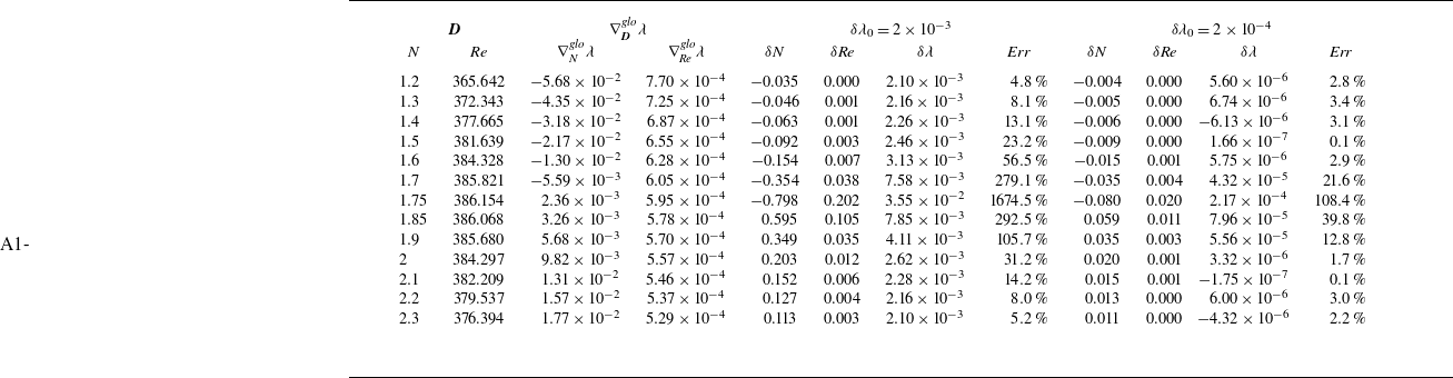
A transition from stabilising to destabilising effect of the magnetic field is shown in zoom 3. The curvature changes dramatically near the extremum point $({\textit{Re}}, N) = (386.3, 1.8)$ . Such a sharp variation observed in the neutral curve arises from the steep gradients of the eigenvalue function $\lambda _r({\textit{Re}}, N)$ , and serves as a sign of strong nonlinearity. The span of $\delta \lambda _r=0.002$ has exceeded the linear range. If linear prediction is still being utilised, the span needs to be reduced to a smaller value, such as $\delta \lambda _r=2\times 10^{-4}$ . The sensitivity calculations along the neutral curve in the vicinity of the extremum point are presented in table 2. With an expected eigenvalue variation $\delta \lambda _0$ , the dimensionless parameter variations are determined by

(4.16) \begin{equation} (\delta {\textit{Re}},\delta N)=\frac {\delta \lambda _0}{(\nabla _{{\textit{Re}}}^{\textit{glo}}\lambda )^2+(\nabla _{N}^{\textit{glo}}\lambda )^2}(\nabla _{{\textit{Re}}}^{\textit{glo}}\lambda, \nabla _{N}^{\textit{glo}}\lambda ). \end{equation}

The exact eigenvalue variation is given by $\delta \lambda =\lambda ({\textit{Re}}+\delta {\textit{Re}},N+\delta N)-\lambda ({\textit{Re}},N)$ and the relative error is defined as $\textit{Err}=||\delta \lambda -\delta \lambda _0||/\delta \lambda _0$ . Two cases for $\delta \lambda _0= 2 \times 10^{-3}$ and $\delta \lambda _0 = 2 \times 10^{-4}$ are considered. Figure 6( $\textit {a}$ ) presents a graphical representation of the sensitivity prediction errors from table 2. When $\delta \lambda _0=2\times 10^{-3}$ , linear prediction is relatively effective in regions far from the extremum $N=1.8$ , such as $N=1.2$ and $N=2.3$ . However, near the extremum, such as $N=1.7$ , $N=1.75$ and $N=1.85$ , linear prediction for $\delta \lambda _0=2\times 10^{-3}$ completely fails. If $\delta \lambda _0$ is reduced to $2\times 10^{-4}$ , the accuracy of linear prediction near the extremum improves with smaller relative errors, and further reduction of $\delta \lambda _0$ will yield better linear prediction. It shows that the effective range of linear prediction near the extremum is much smaller. In other words, nonlinearity is significant in this region. Boujo (Reference Boujo2021) proposed a second-order sensitivity analysis method that improved the predictions of classical linear sensitivity analysis, which could be potentially applied to the present work to enhance sensitivity predictions in the nonlinear region. Figure 6( $\textit {b}$ ) shows the global sensitivity gradients with respect to Re and $N$ . Within this parameter range, the global sensitivity to Re is minimal and remains approximately constant, primarily exhibiting sensitivity to $N$ . The variation in $N$ has a more significant impact on flow instability than that in Re, which means that the magnetic field is the main reason for this phenomenon.

Table 2.

Errors in the predicted eigenvalue variations along the neutral curve in figure 4 near the extremum point $({\textit{Re}},N)=(386.3,1.8)$ . The relative error is defined as $\textit{Err}=||\delta \lambda -\delta \lambda _0||/\delta \lambda _0$ .

Figure 6.

The test for sensitivity calculations on the neutral curve in figure 4 near the extremum point $({\textit{Re}}, N) = (386.3, 1.8)$ . ( $\textit {a}$ ) The global sensitivity of Re and $N$ ; ( $\textit {b}$ ) the relative error for $\delta \lambda _0=2\times 10^{-3}$ and $\delta \lambda _0=2\times 10^{-4}$ .

Figure 4 also provides insights into optimising parameter control strategies with a focus on stability. In practical engineering applications, the task of stabilising an unstable system is often encountered. For example in aircraft engines, flutter stemming from the progressive destabilisation of initial blade vibrations, stands out as a critical failure factor (Yuan & Zhang Reference Yuan and Zhang2023). Nastro et al. (Reference Nastro, Robinet, Loiseau, Passaggia and Mazellier2023) studied low-Reynolds-number flows around NACA 4412 swept wings from the perspective of force sensitivity. They pointed out that a spanwise-homogeneous force suppressed the Hopf bifurcation and stabilised the entire branch of von Kármán modes. In the limit of small amplitudes, passive control via spanwise-wavy forcing produced a stabilising effect similar to that of spanwise-homogeneous control. Khalak (Reference Khalak2002) noted that control can be assessed through a set of similarity parameters like combined mass-damping parameter and compressible reduced frequency parameter. The properties of the global sensitivity gradient provide valuable insights. By controlling the relevant parameters to change along a specific path, the system can transition rapidly, monotonically and robustly from an unstable to a stable state, effectively preventing instability issues such as flutter. To illustrate the control process in detail, the iso- $\lambda _r$ curves in figure 4 are used as a demonstration. Assume the system is initially in an unstable state II at point $\textrm {U}_2$ and needs to be controlled to a stable state at point $\textrm {S}_2$ . There are many paths, such as the ordinary path I or path II (green dashed line), to transition to a stable state. Path I encounters two intersections with the blue contour ( $\lambda _r=0.004$ ). Along this path, the eigenvalue first increases and then decreases, exacerbating the instability before reaching the target parameters. If path II is chosen, the eigenvalue continues to decrease after reaching the same stable state as target. Although it looks better than path I, problem still exits that the system reaches an excessively stable state before gradually destabilising towards the desired state. Along these paths, the eigenvalue changes non-monotonically, which may lead to fluctuations in stability level of the system. Such fluctuations may cause damage to the system as parameters change. However, based on the global sensitivity gradient, the system can be controlled to a desired stable state along the path $\textrm {U}_2\rightarrow U_1\rightarrow C\rightarrow S_1$ , during which the system stabilises monotonically and steeply. Then, by varying parameters along the iso- $\lambda _r$ curve $\textrm {S}_1\rightarrow S_2$ , the system reaches the final desired state while maintaining its stability level. Therefore, an optimal path is established as $\textrm {U}_2\rightarrow U_1\rightarrow C\rightarrow S_1\rightarrow S_2$ (magenta dashed line), ensuring the system’s stability state changes monotonically, steeply and robustly towards the target. In summary, to move the parameter pair from $\textrm {U}_2$ to $\textrm {S}_1$ , multiple iterations are required, using (4.16) to determine the parameter variation $\delta {\textit{Re}}$ and $\delta N$ of each iteration; multiple iterations are also required for the movement $\textrm {S}_1\rightarrow \textrm {S}_2$ along the isoeigenvalue curve, using (3.2) with an additional preset value like $\delta N=0.01$ or other suitable conditions to uniquely determine the parameter variation pair ( $\delta {\textit{Re}},\delta N)$ of each iteration. Therefore, in numerical experiments by DNS, dimensionless parameters can be directly modified within the programme. In practical experiments, based on the expressions of ${\textit{Re}}=U_\infty d/\nu$ and $N=\sigma {\rm d}B^2/\rho U_\infty$ , variations in Re can be achieved by adjusting the free stream velocity $U_\infty$ , while variations in $N$ can be realised by altering the magnetic field strength $B$ . Additionally, the desired dimensionless parameter variations can also be achieved by replacing the fluid material to appropriately adjust properties, such as the density $\rho$ and kinetic viscosity $\nu$ .

Figure 7.

The variation of recirculation length as parameters change along three paths from the start point $\textrm {U}_2$ to the target point $\textrm {S}_2$ . The recirculation length is measured by the zero velocity point in the rear of the sphere.

To evaluate the effectiveness of this control strategy, DNS is conducted with a second-order accurate, consistent and conservative numerical scheme. Detailed information regarding the numerical method can be found in Ni et al. (Reference Ni, Munipalli, Huang, Morley and Abdou2007) and Pan et al. (Reference Pan, Ni and Zhang2018a ). In the flow past a sphere without a magnetic field, as Re increases across the first regular bifurcation ${\textit{Re}}_{c1}\approx 212$ , the flow stability decreases and transitions from an axisymmetric state to a plane-symmetric state. Furthermore, the recirculation length increases accordingly with enlarging the Reynolds number (Bagchi & Balachandar Reference Bagchi and Balachandar2002; Clift, Grace & Weber Reference Clift, Grace and Weber2005). The recirculation length may approximately reflect the stability of the flow, and the longer recirculation length tends to be associated with heightened instability in the flow. Hence, the symmetry and the recirculation length are employed here as indicators of the flow instability for DNS, where the plane-symmetry or the longer recirculation length denote a more unstable state. With these two indicators, figure 7 can show the change of system instability by DNS as the dimensionless parameter point moves along three different paths from the start point $\textrm {U}_2$ to the target point $\textrm {S}_2$ . The horizontal axis, labelled as $l$ , represents the proportion of the parameter point’s travelling distance to the overall length of each respective path. Along path I, although the recirculation length is decreasing, it remains plane-symmetric over an extended range, failing to efficiently transition to an axisymmetric state. Along path II, the recirculation length first decreases and then increases. This non-monotonicity is consistent with the non-monotonic variation in eigenvalues. Along the optimal path, the recirculation length decreases monotonically, which also transitions most rapidly from plane-symmetry to axisymmetry compared with the path II. Furthermore, figure 8 shows the skin friction lines on the sphere surface, which can clearly show flow traces in the rear of the sphere and help us analyse the wake structure (Pan et al. Reference Pan, Zhang and Ni2018b ). The skin friction lines illustrate the axisymmetric state of $\mathrm{S}_1(175.2,25.86)$ , the planar symmetric state of $\mathrm{U}_1(185.1,29.76)$ and the planar symmetric state of $\mathrm{U}_2(190,31)$ that deviates more from axisymmetry in the parameter space $\textit{Re}\mbox{--}$ N. These DNS results are consistent with the analysis from the perspective of the optimal control strategy.

Figure 8.

Skin friction lines on the sphere surface: (a) $\textrm {U}_2$ is ${\textit{Re}}=190$ , $N=31$ , plane-symmetric; (b) $\textrm {U}_1$ is ${\textit{Re}}=185.1$ , $N= 29.76$ , plane-symmetric; (c) $\textrm {S}_1$ is ${\textit{Re}}=175.2$ , $N= 25.86$ , axisymmetric. These three plots correspond to the first three points from left to right on the optimal path in figure 7.

Figure 9.

Global relative sensitivity gradient along the neutral curve versus ( $\textit {a}$ ) $N$ ; ( $\textit {b}$ ) Re.

Figures 9( $\textit {a}$ ) and 9( $\textit {b}$ ), respectively, show the projection onto Re axis and $N$ axis of the global relative sensitive gradient along the neutral curve. Figure 9( $\textit {a}$ ) reflects the dual effects of magnetic field stabilisation ( $\mathrm{P}_0$ to $\mathrm{P}_2$ with negative gradients) and destabilisation ( $\mathrm{P}_2$ to $\mathrm{P}_4$ with positive gradients) corresponding to figure 1(b). The relative sensitivity to the magnetic field drops to nearly zero when $N$ is large. Additionally, the increased field continuously weakens the relative sensitivity of Re. Figure 9( $\textit {b}$ ) clearly reflects that Re in some interval corresponds to two different critical $N$ . Zheng et al. (Reference Zheng, Pan and Ni2023) concluded that the magnetic field stabilises the flow through Joule dissipation while simultaneously destabilising it by exacerbating the shear instability; the former dominates in small $N$ while the latter becomes dominant in large $N$ . Changing Re can obviously alter the recirculation structure of flows past a sphere in the absence of magnetic field. However, the strong magnetic field preserves the fundamental shear structure of the flow, rendering it nearly invariant. On the contrary, the shear structure under small $N$ is unlocked and noticeably affected by Re (Zheng et al. Reference Zheng, Pan and Ni2023). Such a conclusion is supported by the results depicted in figure 9( $\textit {b}$ ) that the relative sensitivity to Re at small $N$ is much greater than that at large $N$ at the same Re.

4.3. Triple-parameter

Figure 10.

The flow configuration for the MHD mixed convection case.

The problem of MHD mixed convection in a two-dimensional periodic channel is considered on the parameter space ${\textit{Re}}\!-\!\textit{Ha}\!-\!{\textit{Gr}}$ , where $\textit{Ha}$ is the Hartmann number. The flow configuration for this problem is shown in figure 10, with the periodic velocity boundary condition $U_{in}=U_{out}$ and the periodic temperature boundary condition $T_{in}=T_{out}$ . The upper and lower boundaries are no-slip wall boundaries with a temperature difference $\Delta T=T_{low}-T_{up}\gt 0$ . The magnetic field $\boldsymbol{B}_0$ is constant and perpendicular to the flow direction. The entire computational domain is $x: [-0.5, 0.5]$ and $y: [-0.1, 0.1]$ . The flow satisfies

(4.17) \begin{align}& \frac {\partial \boldsymbol{U}}{\partial \tau }=-\boldsymbol{U}\cdot \nabla \boldsymbol{U}-\nabla (P+\hat {P})+{\textit{Re}}^{-1}\nabla ^2\boldsymbol{U}+{{\textit{Gr}}}{\textit{Re}}^{-2}T\boldsymbol{e}_y-{\textit{Ha}}{\textit{Re}}^{-1}\boldsymbol{U}, \end{align}

(4.18) \begin{align}&\qquad\qquad\qquad\qquad\qquad\qquad 0=\nabla \cdot \boldsymbol{U}, \end{align}

(4.19) \begin{align}&\qquad\qquad\qquad\qquad \frac {\partial T}{\partial \tau }=-\boldsymbol{U}\cdot \nabla T+{\textit{Re}}^{-1}{{\textit{Pr}}}^{-1}\nabla ^2T, \end{align}

where ${\textit{Re}}=\bar {U}_{in}H/\nu$ is the Reynolds number defined by the average inlet velocity $\bar {U}_{in}$ when the flow is fully developed and reaches a steady state, ${\textit{Gr}}=g\beta \Delta TH^3/\nu ^2$ is the Grashof number, $\textit{Ha}=B_0H\sqrt {\frac {\sigma }{\nu \rho }}$ is the Hartmann number and ${\textit{Pr}}=\nu /\alpha$ is the Prandtl number. Here $\nabla \hat {P}$ is a constant pressure gradient term that drives the flow to the corresponding Re state in a periodic channel. Here, $H, g, \beta, \nu, \alpha, \sigma, \rho, B_0$ represent channel height, gravitational acceleration, coefficient of volume expansion, kinematic viscosity, thermal diffusivity, electrical conductivity, density and magnitude of magnetic induction, respectively. By applying the method presented in this paper, we obtain the linear stability equation (2.6) specifically as

(4.20) \begin{equation} \lambda \!\begin{bmatrix} 1 \!& 0 \!& 0\\ 0 \!& 0 \!& 0\\ 0 \!& 0 \!& 1 \end{bmatrix}\!\begin{bmatrix} \boldsymbol{u} \\ p \\ t \end{bmatrix}\!=\!\begin{bmatrix} \!-\boldsymbol{u}\cdot \nabla \boldsymbol{U}-\boldsymbol{U}\cdot \nabla \boldsymbol{u}-\nabla p+{\textit{Re}}^{-1}\nabla ^2 \boldsymbol{u}+{\textit{Gr}}{\textit{Re}}^{-2}t\boldsymbol{e}_y-\textit{Ha}{\textit{Re}}^{-1}\boldsymbol{u}\\ \nabla \cdot \boldsymbol{u} \\ -\boldsymbol{U}\cdot \nabla t-\boldsymbol{u}\cdot \nabla T+{\textit{Re}}^{-1}{{\textit{Pr}}}^{-}\nabla ^2 t \!\end{bmatrix}\!. \end{equation}

It should be distinguished that $\tau$ represents time and $t$ represents temperature perturbation. The adjoint stability equation (2.19) is specifically written as

(4.21) \begin{align} &\lambda ^*\begin{bmatrix} 1 & 0 & 0\\ 0 & 0 & 0\\ 0 & 0 & 1 \end{bmatrix}\begin{bmatrix} \boldsymbol{u}^\dagger \\ p^\dagger \\ t^\dagger \end{bmatrix}\notag\\&\quad =\begin{bmatrix} \boldsymbol{U}\cdot \nabla \boldsymbol{u}^\dagger -\nabla \boldsymbol{U}\cdot \boldsymbol{u}^\dagger -\nabla p^\dagger +{\textit{Re}}^{-1}\nabla ^2 \boldsymbol{u}^\dagger -\nabla T\cdot t^\dagger -\textit{Ha}{\textit{Re}}^{-1}\boldsymbol{u}^\dagger \\ \nabla \cdot \boldsymbol{u}^\dagger \\ \boldsymbol{U}\cdot \nabla t^\dagger +{\textit{Gr}}{\textit{Re}}^{-2}\boldsymbol{u}^\dagger \cdot \boldsymbol{e}_y+{\textit{Re}}^{-1}{{\textit{Pr}}}^{-1}\nabla ^2 t^\dagger \end{bmatrix}, \end{align}

and the adjoint base flow equation (2.18) is specifically written as

(4.22) \begin{equation} \begin{bmatrix} \boldsymbol{U}\cdot \nabla \boldsymbol{U}^\dagger -\nabla \boldsymbol{U}\cdot \boldsymbol{U}^\dagger +\boldsymbol{u}^*\cdot \nabla \boldsymbol{u}^\dagger -\nabla \boldsymbol{u}^*\cdot \boldsymbol{u}^\dagger -\nabla P^\dagger -\nabla T\cdot T^\dagger -\nabla t^*\cdot t^\dagger\\ +{\textit{Re}}^{-1}\nabla ^2U^\dagger -\textit{Ha}{\textit{Re}}^{-1}\boldsymbol{U}^\dagger \\ \nabla \cdot \boldsymbol{U}^\dagger \\ \boldsymbol{U}\cdot \nabla T^\dagger +\boldsymbol{u}^*\cdot \nabla t^\dagger +{\textit{Gr}}{\textit{Re}}^{-2}\boldsymbol{U}^\dagger \cdot \boldsymbol{e}_y+{\textit{Re}}^{-1}{{\textit{Pr}}}^{-1}\nabla ^2 T^\dagger \end{bmatrix}=\begin{bmatrix} 0 \\ 0 \end{bmatrix}. \end{equation}

Similarly, boundary conditions for the adjoint equations are given by $\Sigma _i\mathcal{J}_i=0$ as $\boldsymbol{u}^\dagger _{in}=\boldsymbol{u}^\dagger _{out},t^\dagger _{in}=t^\dagger _{out},\boldsymbol{u}^\dagger _{up}=\boldsymbol{u}^\dagger _{low}=\boldsymbol{0},t^\dagger _{up}=t^\dagger _{low}=0$ for (4.21), and $\boldsymbol{U}^\dagger _{in}=\boldsymbol{U}^\dagger _{out},T^\dagger _{in}=T^\dagger _{out},\boldsymbol{U}^\dagger _{up}=\boldsymbol{U}^\dagger _{low}=\boldsymbol{0},T^\dagger _{up}=T^\dagger _{low}=0$ for (4.22).

Here we have viscous force $\boldsymbol{F}_v={\textit{Re}}^{-1}\nabla ^2\boldsymbol{U}$ , buoyancy $\boldsymbol{F}_b={\textit{Gr}}{\textit{Re}}^{-2}T\boldsymbol{e}_y$ , Lorentz force $\boldsymbol{F}_L=-\textit{Ha}{\textit{Re}}^{-1}\boldsymbol{U}$ , temperature dissipation $F_t={\textit{Re}}^{-1}{{\textit{Pr}}}^{-1}\nabla ^2T$ and their corresponding perturbed force $\boldsymbol{f}_v={\textit{Re}}^{-1}\nabla ^2\boldsymbol{u},\boldsymbol{f}_b={{\textit{Gr}}}{\textit{Re}}^{-2}t\boldsymbol{e}_y, \boldsymbol{f}_L=-\textit{Ha}{\textit{Re}}^{-1}\boldsymbol{u},f_t={\textit{Re}}^{-1}{{\textit{Pr}}}^{-1}\nabla ^2t$ . The local sensitivity gradients can be quickly written through (2.25) as

(4.23) \begin{align} &\nabla _{{\textit{Re}}}^{loc}\lambda =-\frac {1}{{\textit{Re}}}((\boldsymbol{\boldsymbol{F}}_v+2\boldsymbol{\boldsymbol{F}}_b)^*\cdot \boldsymbol{U}^\dagger +F_t^* T^\dagger +(\boldsymbol{f}_{v}+2\boldsymbol{f}_{b})^*\cdot \boldsymbol{u}^\dagger +f_t^* t^\dagger ), \notag\\ &\nabla ^{loc}_{\textit{Ha}}\lambda = \frac {1}{\textit{Ha}}(\boldsymbol{F}_L^*\cdot \boldsymbol{U}^\dagger +\boldsymbol{f}_L^*\cdot \boldsymbol{u}^\dagger ),\notag\\ &\nabla _{{\textit{Gr}}}^{loc}\lambda =\frac {1}{{\textit{Gr}}}(\boldsymbol{\boldsymbol{F}}_b^*\cdot \boldsymbol{U}^\dagger +\boldsymbol{f}_{b}^*\cdot \boldsymbol{u}^\dagger ), \notag\\ &\nabla _{{\textit{Pr}}}^{loc}\lambda =-\frac {1}{{\textit{Pr}}}(F_t^*T^\dagger +f_t^*t^\dagger ). \end{align}

The total differential of $\lambda =\lambda ({\textit{Re}},\textit{Ha},{\textit{Gr}},{\textit{Pr}})$ is given by

(4.24) \begin{equation} \delta \lambda =\langle \delta {\textit{Re}},\nabla _{{\textit{Re}}}^{loc}\lambda \rangle +\langle \delta \textit{Ha},\nabla _{\textit{Ha}}^{loc}\lambda \rangle +\langle \delta {\textit{Gr}},\nabla _{{\textit{Gr}}}^{loc}\lambda \rangle +\langle \delta {\textit{Pr}},\nabla _{{\textit{Pr}}}^{loc}\lambda \rangle . \end{equation}

In the present study, $\nu =1.88\times 10^{-7}$ and a constant ${\textit{Pr}} = 0.025$ is considered with no variation, i.e. $\delta {\textit{Pr}} = 0$ . Figure 11 shows the results of base flow and perturbation fields at ${\textit{Re}}=5500, \textit{Ha}=5000, {\textit{Gr}}=5.1328\times 10^{7}$ . The structure of the perturbation conforms to Rayleigh–Bénard convection instability (Mistrangelo & Bühler Reference Mistrangelo and Bühler2016). Figure 12( $\textit {a}$ ) illustrates the results of the neutral surface in the triple-parameter space of ${\textit{Re}}\mbox{--}\textit{Ha}\mbox{--}{\textit{Gr}}$ , where ${\textit{Re}} \in [1000, 10\,000]$ and $\textit{Ha} \in [0, 10\,000]$ . Equation (4.24) provides the tangent plane at the point of ${\textit{Re}}=5500,\textit{Ha}=5000,{\textit{Gr}}=5.1328\times 10^{7}$ on the neutral surface. In this case, the neutral surface approaches a plane, resulting in the tangent plane nearly coinciding with it, as shown in figure 12( $\textit {a}$ ). It is noted that adjacent critical points can be fast determined by the linked predict method on the tangent plane within the linear range. Additionally, for no magnetic field cases, increasing ${\textit{Re}}$ results in a rise in the critical ${\textit{Gr}}$ , as shown in figure 12(b). However, figure 12(a) shows that increasing $\textit{Ha}$ can significantly enhance the critical ${\textit{Gr}}$ , indicating that the magnetic field has a strong stabilising effect on the convection within the studied parameter range.

Figure 11.

Contour plots of (a) the base flow $U_x$ ; (b) velocity perturbation $u_x$ ; (c) velocity perturbation $u_y$ ; (d) temperature perturbation $t$ at ${\textit{Re}}=5500$ , $\textit{Ha}=5000$ , ${\textit{Gr}}=5.1328\times 10^{7}$ .

Figure 12.

Neutral surface of triple-parameter MHD mixed convection. (a) The neutral surface in the parameter space ${\textit{Re}}\mbox{--}\textit{Ha}\mbox{--}{\textit{Gr}}$ and the tangent plane at ${\textit{Re}}=5500$ , $\textit{Ha}=5000$ , ${\textit{Gr}}=5.1328\times 10^{7}$ ; (b) the neutral curve in the parameter space ${\textit{Re}}\mbox{--}{\textit{Gr}}$ with $\textit{Ha}=0$ and the tangent represented by red arrows.