


Introduction
Climate change poses a significant threat to the stability of ecosystems, with the potential to drastically reshape the composition and function of oceanic life (Hoegh-Guldberg & Bruno Reference Hoegh-Guldberg and Bruno2010, Doney et al. Reference Doney, Ruckelshaus, Emmett Duffy, Barry, Chan and English2012). Understanding and predicting these ecological impacts has become a crucial focus for scientists, policymakers and environmental managers alike (Kroeker et al. Reference Kroeker, Kordas, Crim, Hendriks, Ramajo and Singh2013, Rudd Reference Rudd2014, IPCC Reference Pörtner, Roberts, Tignor, Poloczanska, Mintenbeck and Alegría2022). In this context, international advisory bodies (IPCC Reference Pörtner, Roberts, Tignor, Poloczanska, Mintenbeck and Alegría2022) have emphasized the importance of identifying species that can serve as early indicators of anthropogenic change. Euthecosomatous pteropods, with their delicate, aragonitic calcified shells, have emerged as key sentinel species for monitoring ocean acidification (Bednaršek et al. Reference Bednaršek, Naish, Feely, Hauri, Kimoto and Hermann2021). Laboratory experiments under controlled conditions and in situ observations have demonstrated that these organisms experience reduced calcification (Comeau et al. Reference Comeau, Gorsky, Jeffree, Teyssie and Gattuso2009, Reference Comeau, Jeffree, Teyssié and Gattuso2010, Lischka et al. Reference Lischka, Budenbender, Boxhammer and Riebesell2011, Gardner et al. Reference Gardner, Manno, Bakker, Peck and Tarling2018, Mekkes et al. Reference Mekkes, Sepúlveda-Rodríguez, Bielkinaitė, Wall-Palmer, Brummer and Dämmer2021) and increased shell dissolution (Manno et al. Reference Manno, Sandrini, Tositti and Accornero2007, Bednaršek et al. Reference Bednaršek, Tarling, Bakker, Fielding, Cohen and Kuzirian2012a, Reference Bednaršek, Naish, Feely, Hauri, Kimoto and Hermann2021, Lischka & Riebesell Reference Lischka and Riebesell2012), especially when shells are damaged (Peck et al. Reference Peck, Oakes, Harper, Manno and Tarling2018) in waters where aragonite saturation is low (ΩAr ≤ 1). Beyond their role as biological indicators, pteropods are integral to high-latitude marine ecosystems and biogeochemical cycles (Manno et al. Reference Manno, Bednaršek, Tarling, Peck, Comeau and Adhikari2017). In the Southern Ocean, for instance, euthecosome pteropods play a pivotal role in ecological networks (Hunt et al. Reference Hunt, Pakhomov, Hosie, Siegel, Ward and Bernard2008, Manno et al. Reference Manno, Bednaršek, Tarling, Peck, Comeau and Adhikari2017, Reference Manno, Giglio, Stowasser, Fielding, Enderlein and Tarling2018, Buitenhuis et al. Reference Buitenhuis, Le Quéré, Bednaršek and Schiebel2019). Pteropods represent an important trophic link between primary producers and higher predators, including fish, seabirds and whales, while also contributing substantially to carbon export through the production and sinking of aragonite shells and faecal pellets (Falk-Petersen & Sargent Reference Falk-Petersen and Sargent2001, Manno et al. Reference Manno, Giglio, Stowasser, Fielding, Enderlein and Tarling2018). Therefore, any shifts in their life history or population dynamics could have far-reaching consequences for ecosystem structure and function.
Studies spanning 16–58 years have examined pteropod abundance across the global ocean to understand how these populations respond to changing environmental conditions. These studies have revealed that, over time, shelled pteropod abundance has declined (Mackas & Galbraith Reference Mackas and Galbraith2012, Beare et al. Reference Beare, McQuatters-Gollop, van der Hammen, Machiels, Teoh and Hall-Spencer2013, Beaugrand et al. Reference Beaugrand, McQuatters-Gollop, Edwards and Goberville2013), stayed stable (Lavaniegos & Ohman Reference Lavaniegos and Ohman2007, Kane Reference Kane2007, Ohman et al. Reference Ohman, Lavaniegos and Townsend2009, Head & Pepin Reference Head and Pepin2010, Loeb & Santora Reference Loeb and Santora2013) and also increased (Ohman et al. Reference Ohman, Lavaniegos and Townsend2009, Kane Reference Kane2011, Mackas & Galbraith Reference Mackas and Galbraith2011, Howes et al. Reference Howes, Stemmann, Assailly, Irisson, Dima, Bijma and Gattuso2015) (Supplementary Material 1). Although these studies have revealed diverse population trends across various geographical regions, they have not provided conclusive evidence linking pteropod abundances to ocean acidification or warming. This lack of clear association between pteropod abundance and anthropogenic impacts may stem from the reliance on broad regional averages to represent environmental conditions, coupled with the tendency to generalize population density by grouping multiple species and life stages. Additionally, logistical challenges in sampling more remote regions have led to a significant imbalance in observational data, with only 15% of pteropod studies conducted in the Southern Hemisphere, compared to 85% in the Northern Hemisphere (Bednaršek et al. Reference Bednaršek, Tarling, Bakker, Fielding, Cohen and Kuzirian2012a, Manno et al. Reference Manno, Bednaršek, Tarling, Peck, Comeau and Adhikari2017). Given these disparities, there is a pressing need for focused, species-specific studies in the Southern Ocean to accurately assess how pteropod populations are responding to environmental changes driven by climate change.
Baseline datasets are essential for tracking population-level changes in response to environmental shifts caused by climate change. These datasets capture the distribution and abundance of organisms prior to significant environmental events, providing a reference point for future comparisons. Establishing such a baseline for pteropod population dynamics and distributions is particularly urgent in high-latitude regions, where the pace of change is most rapid (Negrete-García et al. Reference Negrete-García, Lovenduski, Hauri, Krumhardt and Lauvset2019). These areas are expected to experience the earliest and most intense impacts of ocean change, subjecting organisms to multiple simultaneous environmental stressors (Bromwich et al. Reference Bromwich, Nicolas, Monaghan, Lazzara, Keller, Weidner and Wilson2013, Gutt et al. Reference Gutt, Bertler, Bracegirdle, Buschmann, Comiso and Hosie2015, Huang et al. Reference Huang, Zhang, Zhang, Lin, Hao and Luo2017, Manno et al. Reference Manno, Peck, Corsi and Bergami2022). The Scotia Sea, with its unique biodiversity hotspots, is especially vulnerable. Temperature increases of ~2.3°C in winter and ~0.9°C in summer have already been observed between 1925 and 2006 in waters less than 100 m deep (Whitehouse et al. Reference Whitehouse, Meredith, Rothery, Atkinson, Ward and Korb2008). Moreover, pH declines of up to 0.36 (total scale) are projected for the top 200 m by 2100, with aragonite undersaturation predicted to become ubiquitous down to 200 m throughout the Scotia Sea under the three highest-CO2-emission scenarios (Nissen et al. Reference Nissen, Lovenduski, Brooks, Hoppema, Timmermann and Hauck2024). These trends underscore the importance of baseline data for understanding and mitigating the impacts of climate change on sensitive marine ecosystems.
Many zooplankton species in the Scotia Sea exist at the edge of their environmental tolerance, either as range-edge species that are at the brink of their distribution limits or as endemic species with narrow tolerance thresholds, making them particularly vulnerable to rapid environmental changes (Hogg et al. Reference Hogg, Barnes and Griffiths2011). Previous studies in the northern Scotia Sea have documented Limacina retroversa australis (hereafter L. retroversa), a subpolar species, and Limacina rangii (formerly Limacina helicina), a true polar species, both residing at the extreme southern and northern boundaries of their biogeographical ranges, respectively (Ward et al. Reference Ward, Whitehouse, Brandon, Shreeve and Woodd-Walker2003, Hunt et al. Reference Hunt, Pakhomov, Hosie, Siegel, Ward and Bernard2008, Gardner et al. Reference Gardner, Peck, Bakker, Tarling and Manno2023). The combination of swift environmental shifts and populations living at their range edges makes this region ideal for establishing a baseline of pteropod population dynamics and distributions. However, due to the lack of baseline data, it remains unclear whether pteropod populations are already responding to these environmental changes.
Since the rates of atmospheric CO2 increase and sea-surface warming have accelerated since 1960 (Henson et al. Reference Henson, Beaulieu, Ilyina, John, Long and Séférian2017, Joos & Spahni Reference Joos and Spahni2008), historical samples collected in the Scotia Sea before this period offer a valuable ‘pre-climate change’ baseline. The Discovery expedition, conducted between 1925 and 1951, amassed one of the earliest and most comprehensive collections of plankton samples in the Southern Ocean (Kemp et al. Reference Kemp, Hardy and Mackintosh1929).
This study aims to establish a baseline to define the in situ, species-specific population biogeography and abundances of pteropods. This baseline will be determined using a transect of samples collected by the Discovery investigations in 1929 across the Polar Front between South Georgia and the Falkland Islands. The results of this study represent the earliest, most comprehensive overview of the population dynamics and abundance of pteropods before the impact of anthropogenic change in the frontal zones of the Scotia Sea.
Materials and methods
Sampling stations
A transect of eight stations was sampled between 26 February and 3 March 1929 by the RRS William Scoresby during the Discovery investigations (Fig. 1). The east-west transect stretched 1100 km between the Falkland Islands and South Georgia across the Polar Front. All stations along the transect were completed within 6 days, with the plankton and hydrographical samples at each station being completed in a 12 h window. Stations 518, 520 and 522 were sampled at night, whereas the others were sampled during the day. Station 525 (located between stations 524 and 526 on the transect) was not analysed, as samples at this station were only collected to a depth of 150 m and plankton samples were not available. The station coordinates, dates and times are given in Supplementary Material 2.
An overview of the study region and stations used to define a baseline for pteropod population abundances and dynamics. Dashed lines indicate the position of the Sub-Antarctic Front (SAF), the Polar Front (PF), the Southern Antarctic Circumpolar Current Front (SACCF) and the Southern Boundary of the Antarctic Circumpolar Current (SB-ACC). Positions of the SAF, PF and SB-ACC were taken from Orsi et al. (Reference Orsi, Whitworth and Nowlin1995), while the position of the SACCF was taken from Thorpe et al. (Reference Thorpe, Heywood and Brandon2002).
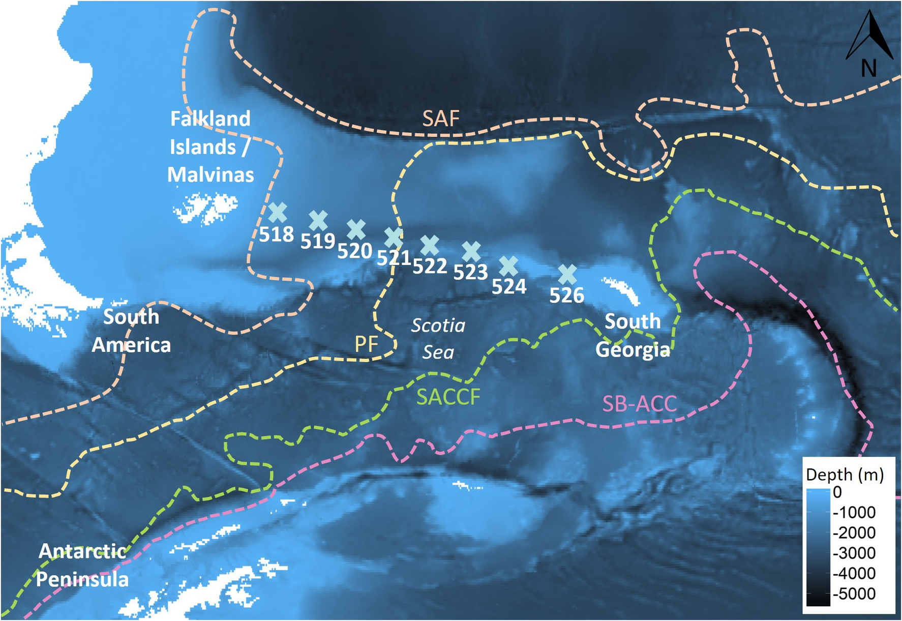
Figure 1 Long description
A bathymetric map uses shades of blue to indicate depth in meters, with a scale bar in the bottom right ranging from 0 at light blue to minus 5000 at dark black.
Landmasses and Regions:
- Northwest: South America and the Falkland Islands / Malvinas.
- Southwest: The tip of the Antarctic Peninsula.
- Center: The Scotia Sea.
- East: South Georgia island.
Research Stations:
A horizontal line of nine light blue X symbols, labeled 518 through 524 and 526, extends from West to East across the Scotia Sea.
Oceanographic Fronts (North to South):
- S A F: An orange dashed line at the top of the map.
- P F: A yellow dashed line that loops around the Scotia Sea and passes between stations 520 and 521.
- S A C C F: A green dashed line running South of the Scotia Sea and South Georgia.
- S B dash A C C: A pink dashed line representing the southernmost boundary, running parallel to the Antarctic Peninsula.
A North arrow is located in the top right corner.
Plankton sample collection
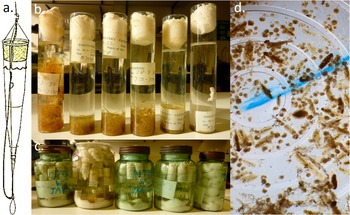
At each station, six depth-discrete plankton samples were obtained using an N70v net (Fig. 2) as follows: 50 m– surface, 100–50 m, 250–100 m, 500–250 m, 750–500 m and 1000–750 m. Details of the net construction are given in Kemp et al. (Reference Kemp, Hardy and Mackintosh1929). Briefly, the N70v was 70 cm in diameter with a collar of ~6 mm knotted mesh, a middle section of 41 threads per inch (equivalent to ~440 μm) and a rear section of 86 threads per inch (equivalent to ~195 μm; Ward et al. Reference Ward, Tarling and Thorpe2014). The net was deployed to the deepest of each of the six depths while open, hauled to the shallowest of the pair at a speed of 1 m/s and then closed via a messenger weight, which triggered the closing mechanism that throttled the net. The nets’ filtration volume was calculated by using the net diameter and the height of the water column sampled. Plankton samples were preserved in buffered formalin for storage in the British Natural History Museum collections (London, UK). The Falkland Islands-South Georgia transect was selected as the organisms were in excellent condition, with no signs of calcium carbonate shell dissolution or damage under inspection with a light microscope (Olympus SZX16 fitted with a Cannon EOS 60D) and under a variable-pressure scanning electron microscope (SEM; TM3000, Hitachi).
An overview of the plankton net, sample storage and inspection technique. a. The N70v plankton net (image from Kemp et al. Reference Kemp, Hardy and Mackintosh1929) used by the RRS William Scoresby during the Discovery investigations between 26 February and 3 March 1929. b. Separate depth horizons were collected from a single station, which c. were stored together in larger jars. d. Samples were inspected using a Doncaster plankton sorting tray.
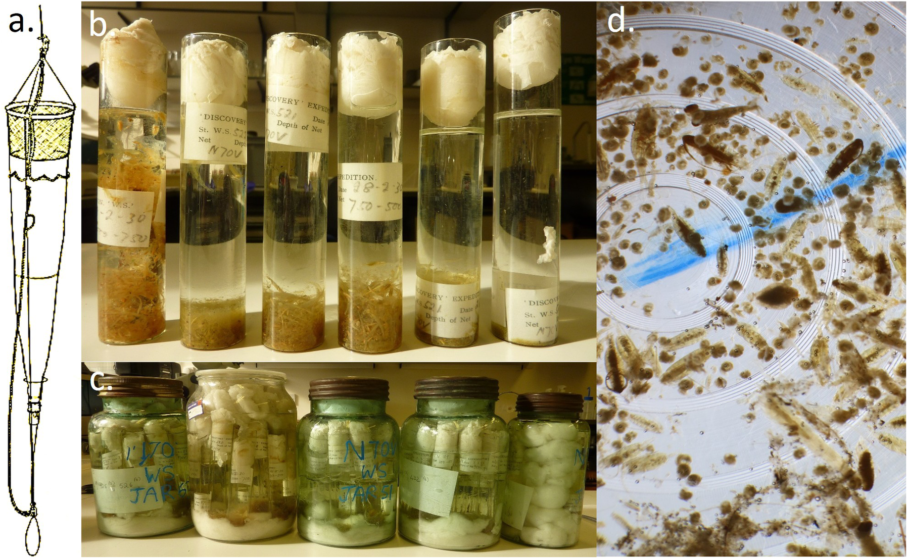
Figure 2 Long description
Panel a, on the far left, is a vertical line drawing of an N 70 v plankton net. It features a conical mesh body suspended by ropes from a top ring, tapering down to a narrow collection bucket at the bottom.
Panel b, at the top center, is a photo of six tall, narrow glass tubes standing in a row. Each tube contains liquid, sedimented biological material at the base, and a large white cotton or wool plug at the top. Labels on the tubes include text such as Discovery Expedition and N 70 V.
Panel c, at the bottom center, shows five large glass jars of varying sizes and tints (clear and green). These jars are filled with the smaller sample tubes from panel b, submerged in preservative liquid. Hand-written blue ink on the jars identifies them as N 70 W S jars.
Panel d, on the right, is a close-up photo of a Doncaster plankton sorting tray. The tray has concentric circular grooves filled with water and numerous small, brownish plankton specimens of varying shapes, including elongated and rounded forms. A blue line is visible across the center of the tray for orientation.
Hydrological data source: temperature, salinity and frontal locations
The original data, along with comprehensive descriptions of instrumentation and sampling methods, are provided in Kemp et al. (Reference Kemp, Hardy and Mackintosh1929). Here, we present a brief summary. Temperature and salinity measurements were determined from water samples collected using Nansen-Pettersson (for depths < 400 m) and Ekman reversing (for depths > 400 m) water bottles. Protected and unprotected reversing thermometers were fitted to the bottles, measuring temperature to a scale of 0.1°C. Salinity was calculated via determining the chloride concentration within a sample by a titration against silver nitrate of a known strength, using potassium chromate as an indicator.
Sampling stations were grouped into two zones: the Polar Frontal Zone and the Antarctic Zone, separated by the Polar Front following Ward et al. (Reference Ward, Tarling and Thorpe2014). The position of the Polar Front was determined through examination of temperature and salinity profiles created using ‘ggplot2{ggplot}’ (Wickham Reference Wickham2009) and potential temperature-salinity profiles. Seawater potential temperature was calculated using ‘oce{swTheta}’ (Kelley et al. Reference Kelley and Richards2017) from the in situ temperatures recorded within the Discovery report’s station list (Kemp et al. Reference Kemp, Hardy and Mackintosh1929) using a reference pressure of 0 dbar. To visualize the thermohaline structure of each sampling station, potential temperature-salinity plots were created using ‘oce{plot.TS}’ (Kelley et al. Reference Kelley and Richards2017). The conditions at each station were compared to the biogeochemical zones defined by Pollard et al. (Reference Pollard, Lucas and Read2002) and the frontal positions approximated by Orsi et al. (Reference Orsi, Whitworth and Nowlin1995). Frontal positions, as defined by Orsi et al. (Reference Orsi, Whitworth and Nowlin1995), were mapped using ‘orsifronts{orsifronts}’ onto bathymetric maps using ‘marmap{plot}’ (Pante & Simon-Bouhet Reference Pante and Simon-Bouhet2013).
Pteropod analysis
Pteropods from the net samples were identified, counted and measured and their shell condition investigated. Pteropod abundance was estimated as number of individuals per m3 based on the volume of water sampled. Since pteropods have a relatively high sinking rate, it is difficult to ensure homogeneous subsamples when using plankton splitting techniques; therefore, samples were analysed in their entirety to prevent any bias (Gardner et al. Reference Gardner, Peck, Bakker, Tarling and Manno2023). Larger pteropods were removed first by hand-picking from a white sorting tray. Afterwards, samples were inspected under a dissection microscope (Olympus SZX16) using a Doncaster plankton sorting tray. Extant euthecosome pteropod species are well described, and identification of unbroken specimens was carried out to species level using Lalli & Gilmer (Reference Lalli and Gilmer1989), van der Spoel (Reference van der Spoel1976) and MSIP (2017). As veligers (larvae) of L. rangii (formally L. helicina) and L. retroversa are difficult to distinguish accurately, individuals smaller than 0.3 mm were classed as Limacina spp. The diameter of each pteropod was measured using the aperture line. On L. rangii and Limacina spp. the aperture line was orientated from the growing edge to the shell edge over the protoconch. On L. retroversa the aperture line passed from the protoconch and down the axis of coiling to the shell edge (also known as spire height; Gardner et al. Reference Gardner, Peck, Bakker, Tarling and Manno2023).
Gymnosome species, having no calcareous shell, contract to varying degrees during the preservation process, meaning body measurements are not reliable, and therefore such data were not taken. Two species of gymnosomes were found along the transect - Spongiobranchaea australis and Clione limacina antarctica (hereafter C. limacina) - with both being specialist predators on thecosome pteropods. These species were pooled together as ‘gymnosomes’, as they occurred at relatively low abundances.
Statistical analysis
Data were analysed using RStudio 0.99.903 (RStudio Team 2016) in R 3.3.2 (R Core Team 2017). All plots presented in this paper were created using ‘ggplot{ggplot2}’ (Wickham Reference Wickham2016). Pteropod abundances (individuals m−3), size distributions and vertical distributions were analysed using generalized linear models (GLMs) implemented in ‘glm{stats}’ (Bolker et al. Reference Bolker, Brooks, Clark, Geange, Poulsen, Stevens and White2008). Models were used to test for differences among hydrographic zones, sampling depths and day/night sampling periods depending on the response variable analysed. Where appropriate, t-tests were used to compare environmental variables between hydrographic zones. Model fit was assessed through inspection of residual distributions and diagnostic plots to ensure assumptions of the selected error structure were met. Following model fitting, significance of explanatory variables was assessed using analysis of deviance and model summaries. Pairwise post hoc comparisons were conducted using estimated marginal means with Tukey adjustment in ‘Emmeans{Emmeans}’ (Lenth Reference Lenth2024), where significant interactions or multiple group comparisons occurred.
Results
Hydrography of the transect
Here, we reanalyse data given in Kemp et al. (Reference Kemp, Hardy and Mackintosh1929) to give the hydrological context of the transect. Surface water down to 80 m was well mixed at each station, with little variation in temperature (maximum range 0.95°C). At station 519 and stations 522–526, from 80 to ~150 m temperatures rapidly decreased (by 0.98– 2.65°C), reaching a temperature minimum, before increasing again (by 1.07–1.90°C) at 400 m depth (Fig. 3). Stations 520 and 521 displayed a unidirectional decline in temperature from the surface to 400 m. There was little variation in salinity down to 150–200 m (maximum range 0.11 ppt). Then, salinity steadily increased from 200 to 1500 m, reaching a maximum of 34.73 ppt. There was little variation in temperature (1.2°C difference) and salinity (maximum range 0.52 ppt) from 400 m to the sea floor at all stations. Stations 518–521 were significantly warmer than stations 522–526 (χ2 22,159 = 31.11, t = 5.82, P < 0.001; Supplementary Material 3).
a. Temperature (°C) and b. salinity profiles of each station (coloured) taken along a transect between the Falkland Islands and South Georgia by the RRS William Scoresby during the Discovery investigations between 26 February and 3 March 1929. Insets detail the temperature and salinity profiles in the top 1000 m. ‘PF’ is the estimated location of the Polar Front. Stations within the Polar Frontal Zone are coloured in blue, while stations coloured in pink are within the Antarctic Zone.
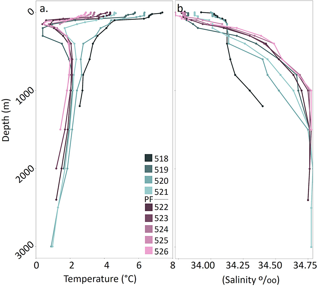
Figure 3 Long description
A two-panel vertical line graph.
Panel a, on the left, displays Temperature in degrees Celsius on the x-axis (0 to 8) against Depth in meters on the y-axis (0 to 3000). The y-axis is inverted with 0 at the top. Multiple colored lines represent different stations. In the top 500 meters, most lines show a sharp decrease in temperature, with several pink and purple lines dipping below 0 degrees Celsius before curving back to stabilize between 1 and 2 degrees Celsius at depths greater than 1000 meters. One dark line remains warmer, staying above 2 degrees Celsius throughout the profile.
Panel b, on the right, displays Salinity in parts per thousand on the x-axis (34.00 to 34.75) against the same Depth y-axis. At the surface, salinity values are dispersed between 33.75 and 34.25. As depth increases to 1000 meters, all lines show a positive trend toward higher salinity. Below 1000 meters, the profiles converge and stabilize near 34.75 parts per thousand.
A legend located between the panels identifies stations 518 through 521 in shades of teal and blue, and stations 522 through 526 in shades of purple and pink. A dashed line labeled P F indicates the Polar Front.
Using the thermohaline structures described earlier, each station was then placed within a hydrographic zone using the definitions of Pollard et al. (Reference Pollard, Lucas and Read2002). There were no stations where salinity decreased with depth; therefore, this transect does not cross into the Sub-Antarctic Zone, which is situated between the Sub-Antarctic Front and the Sub-Tropical Front. At stations 518, 520 and 521, salinity increases and temperature decreases with depth, with no evidence of a subsurface salinity minimum nor a marked subsurface temperature minimum of 2°C. Therefore, these stations were within the Polar Frontal Zone, which is situated between the Sub-Antarctic Front and the Polar Front. There was a clear difference in subsurface temperature between stations 521 and 522, suggesting that the Polar Front is between these stations, which agrees with the average location estimated by Orsi et al. (Reference Orsi, Whitworth and Nowlin1995) (Fig. 1). Stations 522–526 all had a clear subsurface temperature minimum of <2°C, with the underlying water being warmer, placing them within the Antarctic Zone. Interestingly, station 519 also had a subsurface temperature minimum of <2°C; however, its surface temperature and salinity profiles are more like stations within the Polar Frontal Zone. It is possible that station 519 contains an eddy of seawater from the Antarctic Zone.
Pteropod species occurrence, abundance and geographical distribution
A total of 24 108 pteropods were identified, consisting exclusively of two species of thecosome and two species of gymnosome pteropods (Fig. 4). Pteropods that were unidentifiable accounted for 0.1–4.4% of those sampled. Stations within the Polar Frontal Zone (stations 518–521) were dominated by L. retroversa, accounting for 49.1–83.2% of the total pteropod identifiable community (Fig. 5). L. rangii accounted for 0–39.7%, being present on the edge of the Polar Frontal Zone (station 521) and all stations within the Antarctic Zone (stations 522–526).
Pteropod species and groups identified across a transect between the Falkland Islands and South Georgia: a. Limacina rangii, b. Limacina retroversa, c. Limacina species veligers, d. Clione limacina antarctica and e. Spongiobranchaea australis. Images a.–c. are individuals collected by the RRS William Scoresby during the Discovery investigations between 26 February and 3 March 1929. Images d. & e. are of living individuals collected north of South Georgia (28 November 2015, 52.8052°S, 40.08624°W).
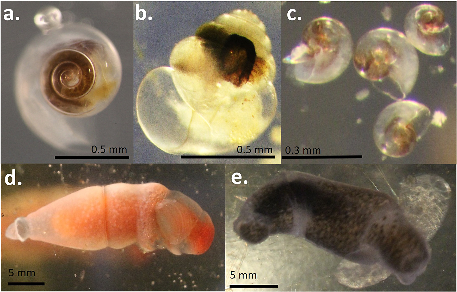
Figure 4 Long description
A multi-panel photo containing five distinct panels labeled a through e.
* Panel a. Top-left. A top-down view of a Limacina rangii shell showing a tight, dark brown spiral at the center of a translucent outer whorl. A scale bar at the bottom right indicates 0.5 mm.
* Panel b. Top-center. A side view of a Limacina retroversa shell with a more globular, translucent structure and a dark internal mass. A scale bar at the bottom right indicates 0.5 mm.
* Panel c. Top-right. Four small Limacina species veligers with iridescent, translucent shells scattered across the frame. A scale bar at the bottom left indicates 0.3 mm.
* Panel d. Bottom-left. A lateral view of a Clione limacina antarctica. It has a torpedo-shaped, translucent body with a prominent orange-red internal organ and a rounded head. A scale bar at the bottom left indicates 5 mm.
* Panel e. Bottom-right. A lateral view of a Spongiobranchaea australis. It has a dark, mottled grey and black elongated body with a slightly curved posture. A scale bar at the bottom left indicates 5 mm.
Percentage abundance of pteropods recorded at each station along a transect between the Falkland Islands and South Georgia. The grey dashed line is the position of the Polar Front during the transect, for which stations 518–521 are in the Polar Frontal Zone and stations 522–526 are in the Antarctic Zone.
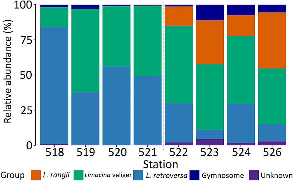
Figure 5 Long description
A stacked bar chart with the Y-axis labeled Relative abundance (%) from 0 to 100 and the X-axis labeled Station with values 518, 519, 520, 521, 522, 523, 524, and 526. A vertical grey dashed line separates stations 521 and 522.
Legend at the bottom identifies five groups:
* L. rangii (orange)
* Limacina veliger (green)
* L. retroversa (blue)
* Gymnosome (dark blue)
* Unknown (purple)
Data trends from left to right:
* Stations 518 to 521 (left of the line): Dominated by L. retroversa (blue) and Limacina veliger (green). L. retroversa starts at approximately 85 percent at station 518 and decreases to 50 percent at station 521. Limacina veliger increases from 15 percent to nearly 50 percent over the same range. Orange segments are absent.
* Stations 522 to 526 (right of the line): L. rangii (orange) appears and becomes a major component, reaching nearly 50 percent at station 526. Limacina veliger (green) remains significant, while L. retroversa (blue) decreases sharply, making up less than 15 percent by station 526. Gymnosome (dark blue) and Unknown (purple) segments are small but consistently present at the top and bottom of the bars respectively in this zone.
Limacina veligers were present at all stations and accounted for approximately half of the pteropods identified (42.9–59.4 %), except at the stations at the extreme ends of the transect, where they were less abundant (station 518: 14.3%; station 526: 39.8%).
C. limacina and S. australis (hereafter grouped as ‘gymnosomes’) contributed 0.7–2.9 % of the identified population in the Antarctic Zone and 1.2–11.1 % in the Polar Frontal Zone. Although gymnosomes were present at all stations, their absolute abundance was significantly higher in the Polar Frontal Zone (15.50 ± 0.18 ind. m−3) than in the Antarctic Zone (χ2 1,7 = 11.39, t = 3.66, P < 0.001, 0.26 ± 0.002 ind. m−3).
The absolute abundance of L. retroversa in the Polar Frontal Zone was significantly higher than in the Antarctic Zone (χ2 1,7 = 8.07, t = 3.11, P = 0.004) and vice versa for L. rangii (χ2 1,7 = 4.27, t = −2.07, P = 0.04; Fig. 6). The absolute abundance of L. retroversa increased from 108.46 ind. m−3 (± 9.38 ind. m−3) at station 518 to 230.84 ind. m−3 (± 25.22 ind. m−3) at station 521. On entering the Antarctic Zone at station 522 the absolute abundance of L. retroversa dropped to 1.15 ind. m−3 (± 0.09 ind. m−3). L. rangii were present in much lower abundances compared to L. retroversa (0.83 ± 0.10 ind. m−3). At the boundary stations between the two zones (stations 521–522), absolute abundances of L. rangii were 0.28 ind. m−3 (± 0.03 ind. m−3) and 0.68 ind. m−3 (± 0.05 ind. m−3), respectively.
The mean number of individuals per m3 for each station along the transect taken by the RRS William Scoresby during the Discovery investigations between 26 February and 3 March 1929. Plot b. is an expanded view of plot a. The grey dashed line is the position of the Polar Front during the transect, for which stations 518–521 are in the Polar Frontal Zone and stations 522–526 are in the Antarctic Zone. Bars denote standard errors.
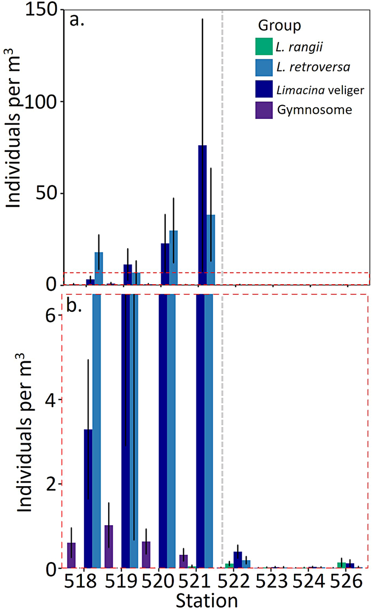
Figure 6 Long description
A vertical multi-panel bar graph with panels labeled a and b. Both panels share a common x-axis labeled Station, with values 518, 519, 520, 521, 522, 523, 524, and 526. A vertical grey dashed line separates station 521 from 522.
Panel a: The y-axis is labeled Individuals per m super 3, ranging from 0 to 150. A legend in the top right identifies four groups: L. rangii (green), L. retroversa (light blue), Limacina veliger (dark blue), and Gymnosome (purple). Data shows a significant peak at station 521 for Limacina veliger (approximately 75) and L. retroversa (approximately 40). Stations 522 through 526 show near-zero values at this scale.
Panel b: This is an expanded view of the lower portion of panel a, indicated by a red dashed box. The y-axis ranges from 0 to 6.
* Station 518: Gymnosome is approximately 0.6, Limacina veliger is 3.3, and L. retroversa is off-chart high.
* Station 519: Gymnosome is approximately 1.0, while Limacina veliger and L. retroversa are off-chart high.
* Station 520: Limacina veliger and L. retroversa are off-chart high, Gymnosome is approximately 0.7.
* Station 521: Limacina veliger and L. retroversa are off-chart high, Gymnosome is approximately 0.3, and L. rangii is near 0.
* Station 522: Values drop significantly. L. rangii is 0.1, Limacina veliger is 0.4, and L. retroversa is 0.2.
* Stations 523, 524, and 526: All groups show values near or below 0.2.
Vertical black lines on the bars denote standard errors.
Limacina veligers had a much greater relative abundance in the Polar Frontal Zone (682.67 ind. m−3, standard error (SE) = 86.03) compared to in the Antarctic Zone (3.45 ± 0.05 ind. m−3; χ2 1,7 = 4.05, t = 1.69, P = 0.044). The absolute abundance of Limacina veligers increased between stations 518 and 521 from 19.75 ind. m−3 (± 1.65 ind. m−3) to 457.34 ind. m−3 (± 68.60 ind. m−3), before declining within the Antarctic Zone (station 522: 2.37 ± 0.15 ind. m−3).
Vertical distribution of pteropods
All of the pteropod groups identified along the Falkland Islands-South Georgia transect were present throughout the water column down to 1000 m. Throughout the transect, pteropods were most abundant at 50–100 m (mean 26.65 ind. m−3).
The number of individuals per m3 of L. retroversa significantly varied with depth (χ2 5,47 = 9.23, P = 0.002; Fig. 7 & Supplementary Material 4) and between day and night (χ2 12,47 = 6.84, z = 6.35, P < 0.001; Fig. 8d). In the daytime peak abundance occurred at 0–50m (z = 8.81, P < 0.001, 15.52 ± 15.21 ind. m−3) and at 50–100 m (z = 6.75, P < 0.001, 37.50 ± 28.79 ind. m−3), while at night L. retroversa was most abundant at 0–250 m (z = 5.76, P < 0.001, 25.00 ± 11.80 ind. m−3) and 500–700 m (z = 4.35, P <0.001, 20.05 ± 19.85 ind. m−3). Furthermore, L. retroversa at 0–50 m (0.42 ± 0.001 mm) in the day were larger than those at 50–1000 m (χ2 13,12797 = 27.96, P <0.001, 0.37 ± 0.01 mm). From day to night there was a shift to smaller L. retroversa at 0–50 m (t = −18.69, P < 0.001, 0.42 to 0.39 ± 0.001 mm) and larger L. retroversa at 50–100 m (t = 25.51, P < 0.001, 0.37 to 0.41 ± 0.001 mm). However, there was no change in the size distribution of L. retroversa below 100 m between day and night (day = 0.38 ± 0.004; night = 0.39 ± 0.001).
The mean number of individuals per m3 with depth across the transect stretching from the Falkland Islands to South Georgia: a. the complete distribution; b. detail of the red dashed box. Bars denote standard error.
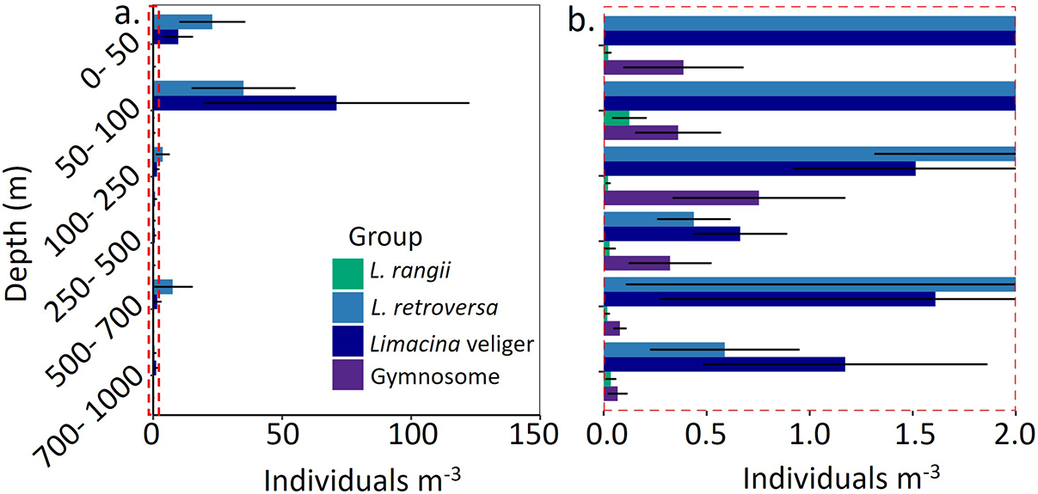
Figure 7 Long description
A two-panel horizontal bar chart. The Y-axis represents Depth in meters, categorized into six intervals: 0 to 50, 50 to 100, 100 to 250, 250 to 500, 500 to 700, and 700 to 1000. The X-axis represents Individuals per m super 3. A legend identifies four groups: L. rangii in green, L. retroversa in light blue, Limacina veliger in dark blue, and Gymnosome in purple.
Panel a shows the full scale from 0 to 150 individuals. The highest concentrations occur in the 50 to 100 meter depth range, where Limacina veliger reaches approximately 70 individuals and L. retroversa reaches approximately 35. Other depth layers show very low values, indicated by a red dashed box near the Y-axis.
Panel b is a detail of the red dashed box, showing a scale from 0.0 to 2.0 individuals.
* At 0 to 50 meters, L. retroversa and Limacina veliger exceed 2.0, while Gymnosome is at 0.4.
* At 50 to 100 meters, L. rangii is at 0.1 and Gymnosome is at 0.35.
* At 100 to 250 meters, L. retroversa and Limacina veliger are between 1.5 and 2.0, while Gymnosome is at 0.75.
* At 250 to 500 meters, L. retroversa is at 0.45, Limacina veliger is at 0.65, and Gymnosome is at 0.3.
* At 500 to 700 meters, L. retroversa and Limacina veliger are between 1.6 and 2.0, while Gymnosome is at 0.1.
* At 700 to 1000 meters, L. retroversa is at 0.6, Limacina veliger is at 1.2, and Gymnosome is at 0.1.
Horizontal black lines on bars indicate standard error.
Shell size and mean number of individuals per m3 of a. & b. Limacina rangii, c. & d. Limacina retroversa, e. & f. Limacina veligers and g. gymnosomes during the day and night. Pteropods were collected across a transect stretching from the Falkland Islands to South Georgia between 26 February and 3 March 1929. One L. rangii being 0.74 mm (at 700–1000 m depth) and two L. retroversa being 3.23 mm (at 0–50 m depth) and 1.5 mm (at 500–700 m depth) were excluded from the plots.
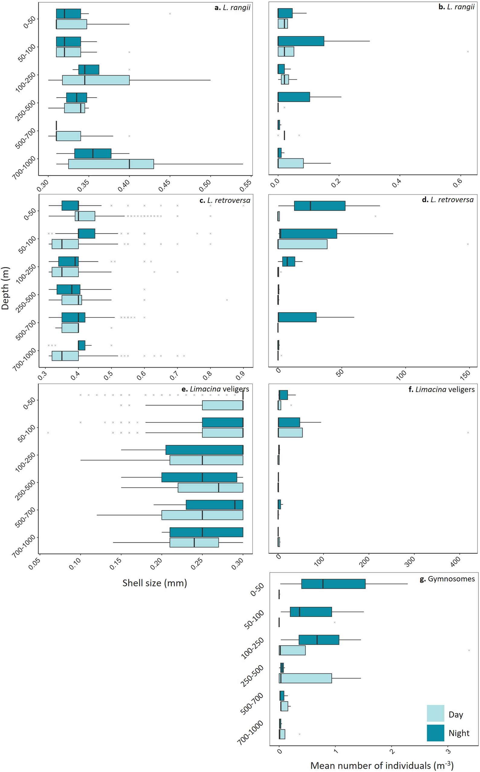
Figure 8 Long description
A multi-panel figure with seven panels labeled a through g. The Y-axis for all panels represents Depth in meters, categorized into six intervals: 0 to 50, 50 to 100, 100 to 250, 250 to 500, 500 to 700, and 700 to 1000. A legend at the bottom right indicates light blue for Day and dark blue for Night.
Panels a, c, and e (left column) show Shell size in millimeters on the X-axis.
* Panel a, Limacina rangii: Shell sizes range from 0.30 to 0.55 millimeters. Sizes are relatively consistent across depths, with a slight increase in median size at the 700 to 1000 meter depth during the day.
* Panel c, Limacina retroversa: Shell sizes range from 0.3 to 0.9 millimeters. Most individuals are concentrated between 0.3 and 0.5 millimeters, with several outliers extending toward 0.9 millimeters.
* Panel e, Limacina veligers: Shell sizes range from 0.05 to 0.30 millimeters. Median sizes generally increase with depth, shifting from approximately 0.25 millimeters at the surface to nearly 0.30 millimeters at 500 to 700 meters.
Panels b, d, f, and g (right column) show Mean number of individuals per cubic meter on the X-axis.
* Panel b, Limacina rangii: Values range from 0.0 to 0.6. The highest density occurs at 50 to 100 meters during the night.
* Panel d, Limacina retroversa: Values range from 0 to 150. Peak density is observed in the top 100 meters, particularly at night in the 0 to 50 meter layer.
* Panel f, Limacina veligers: Values range from 0 to 400. The highest concentrations are found in the 50 to 100 meter layer during both day and night.
* Panel g, Gymnosomes: Values range from 0 to 3. Densities are low overall, with the highest mean numbers occurring in the top 250 meters at night and a notable day peak at 250 to 500 meters.
L. rangii were present down to 1000 m, being most abundant at 50–100 m during both the day (χ2 5,47 = 6.64, t = −5.92, P < 0.001, 0.14 ± 0.12 ind. m−3) and night (χ2 5,47 = 5.43, t = 3.16, P = 0.01, 0.10 ± 0.10 ind. m−3; Fig. 8b). There was no significant difference in the size distribution of L. rangii at any depth between day and night (GLM: χ2 13,112 = 0.48, P >0.001; Fig. 8a).
During the day, Limacina veligers were found at 50–100 m (χ2 12,47 = 0.25, z = 19.42, P < 0.001, 94.57 ± 81.65 ind. m−3), with a smaller number at 0–50 m depth (z = 5.93, P < 0.001, 7.02 ± 5.59 ind. m−3) and a lower abundance at all other depths (> 3.71 ind. m−3; Fig. 7). The number of Limacina veligers at 50–100 m depth during the night was reduced (z = −11.69, P < 0.001, 31.95 ± 81.65 ind. m−3), and this number increased at 0–50 m (z = 2.90, P < 0.001, 14.22 ± 12.32 ind. m−3; Fig. 8f).
There was significant variation in the size of Limacina veligers with depth and between day and night (GLM: χ2 13,10908 = 11.40, P < 0.001; Fig. 8e). In the day, veligers at 0–50 m (0.27 ± 0.001 mm) were larger than those at 500–700 m (t = 3.83, P = 0.01, 0.25 ± 0.01 mm) and at 250–500 m (t = 3.51, P = 0.02, 0.26 ± 0.004 mm). At night, veligers at 0–50 m (0.29 ± 0.001 mm) were larger than those at 700–1000 m (t = 3.99, P = 0.003, 0.25 ± 0.01 mm).
Gymnosomes were most abundant at 100–250 m (χ2 5,47 = 16.47, t = 2.29, P = 0.03, 0.77 ± 0.66 ind. m−3) in the day (Fig. 8g). Although they were present throughout the entire water column, there were very few at the surface during the daytime (0–50 m: 0.002 ± 0.002 ind. m−3). At night, gymnosomes were mostly found at 0–50 m depth (t = 2.04, P = 0.05, 1.03 ± 0.67 ind. m−3).
Following previous estimates of life stage sizes, no adult L. rangii or L. retroversa were collected across the transect, only juveniles and veligers (Lalli & Gilmer Reference Lalli and Gilmer1989).
Discussion
Biogeographical patterns across the Polar Front
Two species of thecosome pteropod were identified along the Discovery investigations’ Falkland Islands to South Georgia transect sampled in 1929: L. retroversa and L. rangii, which are the most common species found in the circumpolar Polar Frontal Zone and Antarctic Zone in contemporary studies (van der Spoel & Dadon Reference van der Spoel, Dadon and Boltovskoy1999, Hunt et al. Reference Hunt, Pakhomov, Hosie, Siegel, Ward and Bernard2008, Bernard & Froneman Reference Bernard and Froneman2009, Howard et al. Reference Howard, Roberts, Moy, Lindsay, Hopcroft, Trull and Bray2011, Roberts et al. Reference Roberts, Howard, Moy, Roberts, Trull, Bray and Hopcroft2011).
Recent investigations have also identified less common Clio pyramidata, Clio recurva, Clio piatkowskii and Heliconoides inflatus within the Southern Ocean (van der Spoel et al. Reference van der Spoel, Newman and Estep1997), species not represented within the Discovery sample set. Limacina inflata are typically found in warmer waters (8–28°C); therefore, it is not surprising that these were not recorded within the northern Scotia Sea. C. piatkowskii have mainly been recorded in the Weddell and Lazarev seas, with very few occurring towards the Polar Front (van der Spoel et al. Reference van der Spoel, Schalk and Bleeker1992, Reference van der Spoel, Dadon and Boltovskoy1999, Hunt et al. Reference Hunt, Pakhomov, Hosie, Siegel, Ward and Bernard2008, Gardner et al. Reference Gardner, Peck, Bakker, Tarling and Manno2023). C. recurva have been recorded in the mesopelagic zone (200–1000 m) between Tasmania and Antarctica (van der Spoel & Dadon Reference van der Spoel, Dadon and Boltovskoy1999, Howard et al. Reference Howard, Roberts, Moy, Lindsay, Hopcroft, Trull and Bray2011). C. pyramidata have often been recorded in the Polar Frontal Zone and Antarctic Zone and might have been expected along the Discovery transect (van der Spoel & Dadon Reference van der Spoel, Dadon and Boltovskoy1999, Hunt et al. Reference Hunt, Pakhomov, Hosie, Siegel, Ward and Bernard2008, Howard et al. Reference Howard, Roberts, Moy, Lindsay, Hopcroft, Trull and Bray2011, Roberts et al. Reference Roberts, Howard, Moy, Roberts, Trull, Bray and Hopcroft2011, Akiha et al. Reference Akiha, Hashida, Makabe, Hattorid and Sasaki2017), yet no specimens were collected in the 1929 samples. The temperatures and salinities recorded along the transect in 1929 were well within the thermal tolerance of most Southern Ocean C. pyramidata formae today (van der Spoel Reference van der Spoel, Schalk and Bleeker1992); therefore, the environmental conditions would have been suitable. Furthermore, the gymnosome S. australis was present in the Discovery investigation samples, a species known to prey preferentially on C. pyramidata (Lalli & Gilmer Reference Lalli and Gilmer1989, Mackas & Galbraith Reference Mackas and Galbraith2011). Although this may suggest that C. pyramidata occurred in the region in 1929, predator occurrence without capture of the primary prey is not uncommon in plankton studies due to patchy prey distributions, temporal mismatches in sampling, low prey abundance or differential net avoidance between species. For example, C. pyramidata are fast and strong swimmers compared to both Limacina species, reaching speeds of ~40 mm/s (Davenport & Bebbington Reference Davenport and Bebbington1990), and so larger individuals are more likely to be able to escape nets than the Limacina species. It is therefore also possible that C. pyramidata was either absent from the sampled water masses at the time of collection or occurred at abundances too low to be detected.
Environmental controls on pteropod biogeography
The Discovery investigations’ transect between the Falkland Islands and South Georgia crossed two major biogeographical zones: the Polar Frontal Zone and the Antarctic Zone, separated by the Polar Front. The position of the Polar Front was similar to its modern-day location, suggesting some stability in its position in this region over the past century (Gille Reference Gille1994, Orsi et al. Reference Orsi, Whitworth and Nowlin1995, Belkin & Gordon Reference Belkin and Gordon1996, Moore et al. Reference Moore, Abbott and Richman1999). A clear shift in pteropod species assemblage occurred between the biogeographical zones, with L. retroversa strongly affiliated with the Polar Frontal Zone, although ranging into the Antarctic Zone, and L. rangii only occurring within the Antarctic Zone. A similar distribution across the Polar Front has also been found in modern-day studies, with L. retroversa being recognized as a subpolar, Polar Frontal Zone species and L. rangii being recognized as a true polar species (Chen & Bé Reference Chen and Bé1964, van der Spoel Reference van der Spoel1967, Reference van der Spoel1976, Lalli & Gilmer Reference Lalli and Gilmer1989, Hunt et al. Reference Hunt, Pakhomov, Hosie, Siegel, Ward and Bernard2008, Akiha et al. Reference Akiha, Hashida, Makabe, Hattorid and Sasaki2017). Therefore, the region between the Falkland Islands and South Georgia is an important monitoring area for biogeographical changes in the distributions of pteropods as it encompasses both the southern range limit of L. retroversa and the northern range limit of L. rangii.
Biogeographical shifts in association with temperature are mainly influenced by the strong relationship to physiological performance and an organism’s optimal thermal niche (Pörtner Reference Pörtner2002, Parmesan & Yohe Reference Parmesan and Yohe2003, Parmesan et al. Reference Parmesan, Gaines, Gonzalez, Kaufman, Kingsolver, Townsend Peterson and Sagarin2005). L. retroversa have been recorded to occupy waters between 5°C and 9°C (< 100 m) in the Argentine Sea (Dadon Reference Dadon1990) and between 2°C and 12°C in the Northern Hemisphere (Bigelow Reference Bigelow1926, Chen & Bé Reference Chen and Bé1964, Beckmann et al. Reference Beckmann, Auras and Hemleben1987, Maas et al. Reference Maas, Lawson and Wang2016). The optimal temperature for L. retroversa is estimated at 2–7°C (van der Spoel & Heyman Reference van der Spoel and Heyman1983), with a thermal maximum of 18°C (Bigelow Reference Bigelow1926). L. retroversa were found to occupy a temperature range of 0.7–6.9°C along the Discovery transect in 1929. L. retroversa individuals occupying temperatures below 2°C are probably functioning suboptimally. From the Discovery investigation transect, L. retroversa were most abundant at 3.8°C, which is within their proposed optimal range. Conversely, L. rangii are true polar pteropods, occupying a lower temperature range of −1.6°C to 5.5°C in the Northern Hemisphere, with a thermal maximum of 7°C (Chen & Bé Reference Chen and Bé1964, van der Spoel & Heyman Reference van der Spoel and Heyman1983). The L. rangii found along the Discovery transect in 1929 occupied temperatures between 0.7°C and 4.2°C, being most abundant at 2.4°C. It is expected that the Polar Front may migrate southwards over the coming decades under continued warming scenarios (Sokolov & Rontoul Reference Sokolov and Rintoul2009), potentially forcing pelagic species to adjust their geographical distributions to remain within their thermal limits (Bates et al. Reference Bates, Orchowska, Garley and Mathis2013). Mackey et al. (Reference Mackey, Atkinson, Hill, Ward, Cunningham, Johnston and Murphy2012) constructed baseline distributions of a wide range of pelagic taxa within the Atlantic sector of the Southern Ocean and Bellingshausen Sea (<100 m) and predicted that, under ~1°C of regional warming, many taxa, including pteropods, may shift polewards. Under such scenarios, the biogeographical range of L. rangii may contract closer to the Antarctic continent, while conditions suitable for L. retroversa may expand and extend southwards. Such distributional changes may also have broader biogeochemical implications, as pteropods contribute substantially to carbon export through the production and sinking of aragonitic shells and faecal pellets (Manno et al. Reference Manno, Giglio, Stowasser, Fielding, Enderlein and Tarling2018). Shifts in the abundance and distribution of dominant pteropod species could therefore alter the spatial patterns of carbonate export and carbon cycling within the Southern Ocean.
As well as the strong relationship between temperature and physiological performance, other ecological aspects also control biogeographical distributions, including species interactions, trophodynamics and community composition (Parmesan & Yoho Reference Parmesan and Yohe2003, Richardson Reference Richardson2008). Gymnosomes were present at every station along the Discovery transect in 1929, contributing 1.17–11.11% of the pteropod population in the Polar Frontal Zone and 0.65–2.90% of the pteropod population in the Antarctic Zone. The absolute abundance of gymnosomes was also lower in the Antarctic Zone in comparison to in the Polar Frontal Zone. Physiologically, gymnosomes have a much higher thermal tolerance than their thecosome pteropod prey, with C. antarctica’s range being −1.7°C to 15.2°C and S. australis’s range being 2.3–13.2°C (van der Spoel Reference van der Spoel1976, Dadon & Chauvon Reference Dadon and Chauvin1998, Dymowska et al. Reference Dymowska, Manfredi, Rosenthal and Seibel2012). In the Discovery investigations’ samples, gymnosomes were found in waters between 0.68°C and 6.90°C, which is well within this tolerance range. It is improbable, therefore, that the distribution of gymnosomes was controlled by temperature along the Discovery transect, which was more correlated with L. retroversa and L. rangii distributions. Gymnosomatous pteropods are highly specialized predators that have evolved in concert with their thecosomatous relatives, which are their exclusive prey item (Conover & Lalli Reference Conover and Lalli1972, Gilmer & Lalli Reference Gilmer and Lalli1990, Seibel et al. Reference Seibel, Dymowska and Rosenthal2007). Therefore, the distribution of gymnosomes is most likely to align with the abundance distribution of their prey items.
The Discovery transect has no freshwater or sea-ice influence; therefore, it is improbable that salinity variability would be a major controlling factor for pteropod distributions. L. retroversa were collected within salinities ranging from 33.90 to 34.72 and L. rangii were collected within salinities ranging from 33.80 to 34.70. L. retroversa are euryhaline, meaning that they have a wide tolerance of salinities (30.1–36.0). The tolerance window of L. rangii is narrower, being 33.55–36.14, rendering them more vulnerable to freshwater inflow, which could be an influencing factor for more southern populations, where there is more sea ice present, but not between the Falkland Islands and South Georgia (Gilmer Reference Gilmer1974, Kobayashi Reference Kobayashi1974, Dadon Reference Dadon1990, Manno et al. Reference Manno, Morata and Primicerio2012).
Vertical distribution and migration of pteropods
Pteropods are mainly described as an epipelagic species (upper 200 m), co-occurring with phytoplankton that form a major part of their diet (Atkinson et al. Reference Atkinson, Shreeve, Pakhomov, Priddle, Blight and Ward1996, Hunt et al. Reference Hunt, Pakhomov, Hosie, Siegel, Ward and Bernard2008, Akiha et al. Reference Akiha, Hashida, Makabe, Hattorid and Sasaki2017, Wang et al. Reference Wang, Hunt, Liang, Pauly and Pakhomov2017). Pteropod studies most commonly focus on the upper 200 m of the water column, where sampling effort is concentrated. However, a growing number of studies are finding pteropods within the mesopelagic zone (200–1000 m), with a much more varied diet (Kobayashi Reference Kobayashi1974, Wormuth Reference Wormuth1981, Bednaršek et al. Reference Bednaršek, Tarling, Bakker, Fielding, Cohen and Kuzirian2012a, Hunt et al. Reference Hunt, Pakhomov, Hosie, Siegel, Ward and Bernard2008). Bednaršek et al. (Reference Bednaršek, Tarling, Bakker, Fielding, Cohen and Kuzirian2012a) collated a large database of global pteropod abundance, with pteropods recorded at depths down to 2000 m. The highest biomass of pteropods along the Discovery investigations’ transect was found at 0–200 m, decreasing to 1000 m, although there were distinct regional differences. We found that all pteropod groups were present down to 1000 m, emphasizing the need to sample down to >1000 m rather than concentrating on the epipelagic zone, as this may result in underestimation of pteropod population abundances and distributions. Since the Discovery investigations only sampled to 1000 m, it is possible that there were pteropods below this depth, as the sea floor was between 1434 and 3674 m deep.
Life stage-specific depth distributions
The veligers of Limacina species (< 0.3 mm), unlike juveniles, were predominantly present within the surface (< 100 m) across the entire transect, with no evidence of vertical movement between day or night. Veligers are probably constrained to the surface as they have limited swimming capabilities, relying on ciliated velums for locomotion rather than the characteristic wings that develop in the juvenile stage (Lebour Reference Lebour1932, Lalli & Gilmer Reference Lalli and Gilmer1989, Howes et al. Reference Howes, Bednaršek, Budenbender, Comeau, Doubleday, Gallager, Hopcroft, Lischka, Maas, Bijma and Gattuso2014). As veligers have limited vertical movement, the benefit of residing in the food-rich surface layers, allowing increased growth rates (Dadon & de Cidre Reference Dadon and de Cidre1992), is greater than the threat of predation. However, once individuals develop wings, they utilize the entire water column sampled (<1000 m), avoiding the threat of predation by gymnosomes while maximizing the time spent within food-rich surface layers.
Juvenile L. rangii and L. retroversa, with their developed wings, exhibit more mobility through the water column. Juvenile L. retroversa were most abundant between 50 and 100 m during the day, while at night their distribution was more dispersed, with some individuals migrating upwards to 0–50 m as well as descending to 500–700 m. Similarly, L. rangii were also most abundant between 50 and 100 m during the day, with a second peak at 700–1000 m. At night, most the distribution of L. rangii shifted towards shallower depths, with the highest abundance remaining within the 50–100 m interval. This differential depth distribution between day and night suggests that juveniles of both L. rangii and L. retroversa undertake a weak vertical migration. In general, vertical migration to the surface at night reduces the risk of predation by visual predators while feeding where food is most abundant (Gliwicz Reference Gliwicz1986, Hays Reference Hays2003). Previous studies have also found an increase in the abundance of L. retroversa in the upper 50 m during the night (Chan & Bé Reference Chen and Bé1964, Wormuth Reference Wormuth1981, Beckmann et al. Reference Beckmann, Auras and Hemleben1987). Surface densities of L. rangii have also been observed to increase at night (Atkinson et al. Reference Atkinson, Shreeve, Pakhomov, Priddle, Blight and Ward1996, Hunt et al. Reference Hunt, Pakhomov, Hosie, Siegel, Ward and Bernard2008, Steinberg et al. Reference Steinberg, Ruck, Gleiber, Garzio, Cope and Bernard2015). Although we show that both L. rangii and L. retroversa shift their vertical distribution at night, individuals were still most abundant at the surface during the day, indicating that illumination is not the main control on vertical distribution.
All individuals of L. rangii and L. retroversa identified (maximum shell size < 0.8 mm) were juveniles, except for two adult L. retroversa (3.23 and 1.50 mm; following Lalli & Gilmer Reference Lalli and Gilmer1989). Adults with well-developed wings are much more mobile through the water column (Adhikari et al. Reference Adhikari, Webster and Yen2016), and it may be possible that few adult L. rangii and L. retroversa were collected in the Discovery nets as they were at depths greater than 1000 m or because they were able to avoid the nets by being faster and stronger swimmers than juveniles and veligers. As adult pteropods were not sufficiently represented, further work on the vertical and biogeographical range of the adult stages is needed.
By comparing the depth distribution of gymnosomes and juvenile Limacina, it appears that Limacina avoid depths where gymnosomes are more abundant. Alternatively, this observation may be due to Limacina at this depth being predated on. Whether this observation is a cause or effect, it supports the idea that vertical migration by Limacina, similarly to many other migrators, is most probably undertaken as a predator avoidance behaviour (Lampert Reference Lampert1993). Gymnosomes displayed the clearest vertical migration from the deeper layers in the day to the surface at night. During the day, gymnosomes were less abundant between 0 and 100 m, while L. rangii and L. retroversa were most abundant. Furthermore, there were very few gymnosomes at 700–1000 m, which could explain the secondary peak abundance of L. rangii at these depths. At night, the gymnosomes moved to the upper 0–250 m. Although both Limacina species also moved upwards, both also congregated deeper in the water column (L. retroversa: 500–700 m; L. rangii: 250–500 m), reducing the vertical overlap with gymnosomes. It is probable that predation risk is a stronger factor in controlling juvenile pteropod distribution than food supply, as adult pteropods are able to capture a variety of food sources within their large mucous nets.
Both gymnosomes and thecosome pteropods are themselves important food sources to a host of other organisms, including numerous carnivorous zooplankton, fish, mammals and birds (Levasseur et al. Reference Levasseur, Keller, Bonneau, D’Amours and Bellows1994, Karnovsky et al. Reference Karnovsky, Hobson, Iverson and Hunt2008, Pomerleau et al. Reference Pomerleau, Lesage, Ferguson, Winkler, Petersen and Higdon2012, Murphy et al. Reference Murphy, Adhikari, Webster and Yen2016, Litz et al. Reference Litz, Miller, Copeman, Teel and Weitkamp2017). As many of these are visual predators, it would be beneficial for both types of pteropod to avoid surface layers during the day. However, the juvenile stages of both Limacina species primarily remain in the upper 200 m during the daytime, whereas gymnosomes migrate deeper, suggesting other factors are also controlling their distribution. C. limacina lack an escape response from predators, whereas Limacina can detect turbulence from predators and rapidly sink to avoid them (Gilmer & Lalli Reference Gilmer and Lalli1990, Borrell et al. Reference Borrell, Goldbogen and Dudley2005). Therefore, C. limacina may experience a greater threat from predation and avoid the photic zone during the day. Gymnosomes and thecosome pteropods have coevolved highly specialized predation and evasion techniques in a predator-prey arms race (Seibel et al. Reference Seibel, Dymowska and Rosenthal2007). Because of this co-evolution, it would be more beneficial for Limacina to avoid gymnosomes and reside in the food-rich surface layers during the day, despite the threat from visual predators.
Concluding remarks and summary
This study contributes fundamental baseline data on the biogeographical range of pteropods before the impact of anthropogenic change in the Scotia Sea. This baseline is crucial for future comparisons and for interpreting changes of pteropod ranges. We show that the northern range of L. rangii is bounded by the Polar Front, with the northern Antarctic Zone representing the trailing edge of L. rangii’s biogeographical range. As the abundance of L. retroversa drops south of the Polar Front, the northern Antarctic Zone marks the southern, leading edge of its range. It is probable that the biogeographical ranges of both Limacina species are limited by their thermal tolerances. In contrast, gymnosomes were found across the entire transect, reflecting the abundance of their Limacina prey rather than temperature, owing to their wide thermal niche and close predator-prey relationship with thecosome pteropods. The differential depth distribution between day and night suggests that both L. rangii and L. retroversa undertake weak vertical migration. This vertical migration was not only in response to illumination but may also represent a predator-avoidance behaviour, as vertical segregation between gymnosomes and their Limacina prey was identified. Vertical distribution was also dependent on life stage, with veligers residing in the upper 100 m and juveniles being dispersed across all sampling depths (0–1000 m). The absence of adult Limacina also suggests that larger individuals may migrate to depths greater than 1000 m, but we cannot exclude the possibility that some individuals were able to avoid the plankton nets. Future resampling of this historical transect would provide a valuable opportunity to assess long-term changes in pteropod biogeography, population structure and vertical distribution across the Polar Front. Incorporating this region into sustained monitoring programmes could help track ecosystem responses to ongoing environmental change and improve predictions of future Southern Ocean ecosystem dynamics.
The enduring legacy of these historical data highlights their invaluable role in tracking long-term ecological changes, offering a unique reference point for assessing the impacts of ongoing climate change on pteropod populations and the ecosystems that they support.
Supplementary material
To view supplementary material for this article, please visit http://doi.org/10.1017/S0954102026100893.
Acknowledgements
We would like to acknowledge the captain, officers, crew and scientists aboard the RRS William Scoresby during the Discovery investigations.
Author contributions
JG carried out the data collection, with support from GT and CM. JG wrote the manuscript, with support from VP, DB, GT and CM. All authors contributed to the article and approved the submitted version.
Competing interests
The authors declare none.



 Open access

