I. INTRODUCTION
The nanoindentation test has been widely used to measure the mechanical properties of materials at small length scales, which is especially useful for thin films and nanostructured materials.Reference Doerner and Nix1–Reference Gouldstone, Chollacoop, Dao, Li, Minor and Shen7 The basis for the nanoindentation test is that the projected contact area can be estimated from the load–displacement curve, rather than by imaging the indentation impression like a microhardness test.Reference Doerner and Nix1, Reference Oliver and Pharr2 The Oliver–Pharr methodReference Oliver and Pharr2 has been commonly adopted to determine the projected contact area and extract the hardness and elastic modulus from the load–displacement curves. In the classic Oliver–Phar method, knowing the loading force P at indentation depth h, the contact depth h c is estimated by h c = h − ∈ ⋅ P / S, in which the stiffness S = dP / dh is the initial slope of the unloading curve and ε is a constant related to the geometry of the indenter (ε = 0.75 is the commonly used empirical valueReference Oliver and Pharr5). For a Berkovich indenter, the projected contact area A c is calculated as  . Then, the hardness H can be determined with H = P / A c.
Materials with a low work-hardening rate normally pile up, whereas those with a high work-hardening rate sink in.Reference Tabor8–Reference Mata and Alcala11 The variation in contact area due to pile-up or sink-in produces errors in the Oliver–Pharr method. Once pile-up or sink-in occurs, the projected contact area may be underestimated or overestimated, respectively. Then, the errors generated in the calculation of the projected contact area leads to a higher or lower hardness than its true value. Therefore, it is important to understand how greatly the contact profile varies with the material properties during nanoindentation and how large will be the errors in the projected contact area and hardness for different materials.
Finite element models have been widely used to study the pile-up and sink-in phenomena for many materials.Reference Giannakopoulos, Larsson and Vestergaard12–Reference Taljat and Pharr18 The indenter has been most commonly modeled as a two-dimensional (2D) equivalent cone with an apex angle of 70.3°, which gives the same relationship between the projected contact area and the indentation depth as a Berkovich indenter.Reference Bolshakov and Pharr15, Reference Dao, Chollacoop, Van Vliet, Venkatesh and Suresh17 It has been shown that the work-hardening rate n and the ratio of yield stress to elastic modulus σ y/E are the dominant parameters affecting the contact profile.Reference McElhaney, Vlassak and Nix14, Reference Bolshakov and Pharr15 However, the 2D axisymmetric models cannot reproduce the nonuniform plastic flow caused by the geometric features of the Berkovich indenter, which cannot be coarsely idealized to the 2D case. From both experimental and numerical results, it was evident that the material piles up the least on the edges and the most at the mid-plane of the facets of the indenter.Reference Giannakopoulos, Larsson and Vestergaard12–Reference McElhaney, Vlassak and Nix14, Reference Randall19 It has been pointed out that the Berkovich indenter is not equivalent to the 70.3° conical indenter in terms of the curvature of the loading curve.Reference Swaddiwudhipong, Hua, Tho and Liu20 Therefore, three-dimensional (3D) modeling of the Berkovich indenter is required to deal with its 3D geometric features. By applying 3D modeling and simulation, the projected contact area can not only be estimated from the load–displacement curve using the classic Oliver–Pharr method but can also be directly determined according to the contact pressure on the surfaces of the finite elements contacted. These two methods can be both applied in post-processing the results of a 3-D finite element simulation and thus the errors in the projected contact area obtained with the Oliver-Pharr method can be evaluated for materials exhibiting pile-up or sink-in behaviors.
In this study, a 3D finite element model is developed and applied to simulate the Berkovich nanoindentation for a wide range of elastoplastic materials, and this is also compared with an equivalent 2D conical indentation model. The variations in the contact profile are correlated with two material parameters: the work-hardening rate n and the ratio of the yield stress to the elastic modulus σ y/E. Then, the plastic deformations in the indentation region are investigated to explain the effects of the mechanical properties on the contact profile. Finally, the errors in the projected contact area estimated through the Oliver–Pharr method are evaluated for the materials with different n and σ y/E.
II. MODEL DESCRIPTION
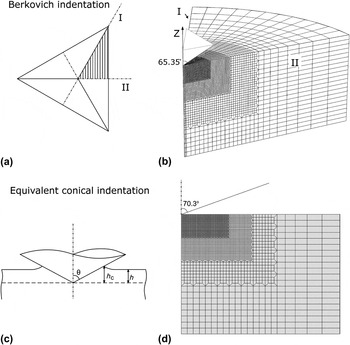
A 3D finite element model was developed to simulate the Berkovich nanoindentation with the commercial finite element program—Abaqus V6.8. Considering the 6-fold symmetry of the Berkovich indenter,Reference Larsson, Giannakopoulos, SÖderlund, Rowcliffe and Vestergaard13 only one-sixth of a cylindrical specimen was modeled with plane-symmetry boundary conditions applied in planes I and II, as shown in Fig. 1(a). The specimen had a thickness of 2.0 μm and a radius of 4.0 μm. The bottom of the specimen was fixed as if it was located above a rigid substrate. A gradient mesh by using 40140 C3D8R elements in total, featuring a refined mesh in the indentation region, was developed to model the specimen, which is shown in Fig. 1(b). A rigid surface was used to represent a perfect Berkovich indenter with a half angle of 65.35°. The contact between the indenter and the specimen was assumed to be hard contact and frictionless. The indenter penetrates into the specimen along the z-direction under quasistatic and isothermal conditions, consisting of loading, holding, and unloading phases. The maximum indentation depth was set to 0.2 μm, which was 10% of the total thickness of the specimen. In addition, a 2D axisymmetric model was also built to compare with the proposed 3D model. All of the setups were equivalent in these 2D and 3D models, except that a rigid conical indenter with half angle of 70.3° was used in the 2D model, as shown in Fig. 1(d).
(a) Symmetry of the Berkovich indenter, (b) mesh of three-dimensional (3D) Berkovich indentation model, (c) illustration of the conical indentation, and (d) mesh of the equivalent two-dimensional (2D) model.

The material of the specimen was assumed to be elastoplastic, following the von Mises yielding criteria. A power-law work-hardening behavior was prescribed for plastic deformation, which approximates the work-hardening behavior of most metals.Reference Dieter21 The true stress–true strain curve is given as
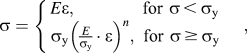
in which σ y is the yield stress and n is the work-hardening rate. According to the dimensional analysis,Reference Cheng and Cheng22 the contact profile in the nanoindentation depends on the σ y/E, n, ν, and the half angle θ. In the current simulation, the half angle of the indenter and the Poisson’s ratio of the specimen were kept unchanged at 65.35° and 0.3, respectively. Hence, the σ y/E and n are the only parameters that affect the contact profile. To further simplify the numerical problem, Young’s modulus E = 210 GPa was used in all simulations, but the yield stress was varied systematically from 52.5 to 1680.0 MPa, corresponding to ratios of σ y/E from 0.25 × 10⁻³ to 8.0 × 10⁻³. The work-hardening rate n was varied from 0.0 to 0.5. In general, this range of σ y/E and n covers the mechanical properties of most metals.Reference Dieter21
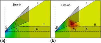
By postprocessing the results obtained from the nanoindentation simulations, the contact areas were determined according to the contact pressure recorded in the model, assuming that the areas in contact have a nonzero contact pressure. These contact areas must be projected to the basal plane of the Berkovich indenter, which is commonly used as the projected contact area in the hardness calculation.Reference Doerner and Nix1, Reference Oliver and Pharr2 In the 2D axisymmetric model, the contact depth h c is defined as the vertical distance of the contact region, as shown in Fig. 1(c). For the 3D Berkovich nanoindentation, the maximum pile-up or sink-in occurs on the mid-plane of facet (plane II), whereas the edge side (plane I) usually has minimal pile-up or sink-in.Reference Lim and Chaudhri9, Reference Giannakopoulos, Larsson and Vestergaard12, Reference Larsson, Giannakopoulos, SÖderlund, Rowcliffe and Vestergaard13, Reference Randall19, Reference Tsui and Pharr23 Hence, the contact depth h c is defined as the vertical distance of the contact profile on the mid-plane of facets in the 3D model, as shown in Fig. 2. For comparison, the contact depth was also extracted from the load–displacement curve by using the Oliver–Pharr method as  . Then, the projected contact area corresponding to the contact depth
 was calculated as
 .
Illustration of h c defined in the 3-D model for both (a) sink-in and (b) pile-up.

III. RESULTS AND DISCUSSION
A. Comparison of the contact depth in 2D and 3D models
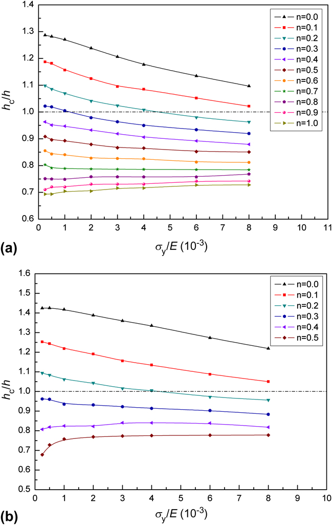
According to the dimensional analysis,Reference Dao, Chollacoop, Van Vliet, Venkatesh and Suresh17, Reference Cheng and Cheng24h c/h is a dimensionless function of σ y/E, n, ν, and θ. As ν and θ are fixed in the current simulations, the ratio of h c/h is only depending on σ y/E and n. The value of h c/h is greater than unity when pile-up occurs and smaller than unity when sink-in occurs. The variation of h c/h with respect to σ y/E and n obtained from the 3D model is shown in Fig. 3(a). Materials with a low work-hardening rate are prone to pile-up, whereas those with a high work-hardening rate are more likely to sink in. This is consistent with experimentsReference Lim and Chaudhri9, Reference McElhaney, Vlassak and Nix14, Reference Randall19, Reference Tsui and Pharr23 and other simulation results.Reference Giannakopoulos, Larsson and Vestergaard12, Reference Larsson, Giannakopoulos, SÖderlund, Rowcliffe and Vestergaard13
Variation of h c/h with respect to σ y/E and n obtained from (a) 2D and (b) 3D models.
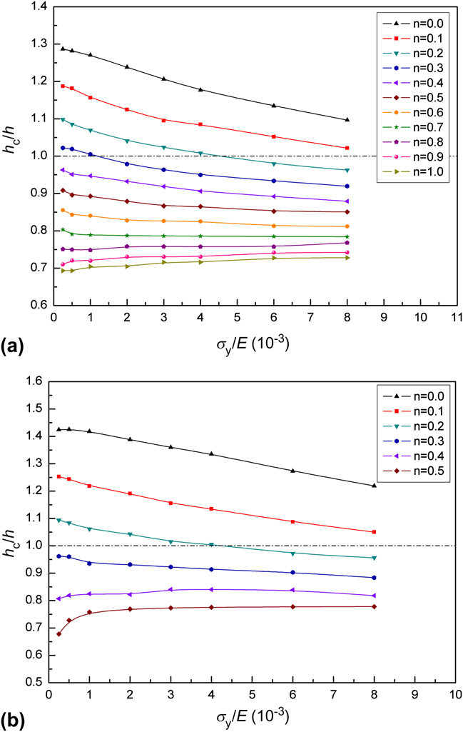
The results from the 3D model show that the contact depth h c/h decreases with increasing σ y/E when n is between 0.0 and 0.3 (referred as the negative correlation), and increases with increasing σ y/E when n is higher than 0.3 (referred as the positive correlation). To the best knowledge of the authors, such a positive correlation between σ y/E and n has not been discovered by 2D axisymmetric models in literatures. However, the positive correlation between h c/h and σ y/E does not apply to all sink-in materials. It is noted that sink-in also happens to materials with n = 0.3, but the h c/h decreases with increasing σ y/E. This suggests that the positive correlation only occurs in materials with a high work-hardening rate. The transition from the negative correlation to the positive correlation takes place between n = 0.3–0.4.
The results from the 3D model appears contradictory with those from previous 2D axisymmetric modelsReference Mata and Alcala11, Reference Cheng and Cheng24 in which the h c/h decreases when σ y/E is increasing for n between 0.0 and 0.5. Though the h c is defined on the mid-plane of facet (plane II), the qualitative relationship between h c/h and σ y/E is not affected by the trivial differences in definition between the 2D and 3D models. However, it is noticed that the decreasing rate of h c/h with increasing σ y/E becomes smaller when n increases from 0.0 to 0.5 in previous 2D axisymmetric models.Reference Mata and Alcala11, Reference Cheng and Cheng24 For comparison, we have also modeled the conical indentation with an equivalent 2D axisymmetric model and extended the range of n up to 1.0. Figure 3(b) shows the h c/h for materials in the range of σ y/E = 0.25–8.0 × 10⁻³ and n = 0.0–1.0 obtained from the 2D axisymmetric model. The data from the current 2D axisymmetric model have similar values and trends as the data in the range of σ y/E = 0.25–8.0 × 10⁻³ and n = 0.0–0.5 in the previous works,Reference Mata and Alcala11, Reference Cheng and Cheng24 though plotted with different axis scales. Since the range of n is extended up to 1.0, the positive correlation between h c/h and σ y/E is observed for n > 0.7 through the 2D simulations. It suggests the positive correlation between h c/h and σ y/E happens for high work-hardening materials, which can also be captured by using 2D models.
B. Plastic deformation in the indentation region
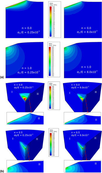
The plastic deformation in the indentation region needs to be investigated to explain why opposite relationships between h c/h and σ y/E exist at low and high work-hardening rates. Figure 4 shows the distribution of equivalent plastic strains for four representative materials from both the 2D and 3D models. For both the conical and Berkovich indentations, the maximum plastic strain occurs in the regions immediately under the indenter. However, in Berkovich indentation, the equivalent plastic strain distributes nonuniformly on the facet of the tip; the edge side has the maximum equivalent plastic strain, whereas the mid-plane of the facet has much smaller equivalent plastic strains.
Contours of equivalent plastic strains at 0.2 μm indentation depth for four extreme materials: (a) 2D conical indentation and (b) 3D Berkovich indentation.

The maximum equivalent plastic strain reduces significantly as the work-hardening rate increases. More importantly, two distinct types of plastic deformation are observed for the materials with low and high work-hardening rates, respectively. For materials with n = 0, the plastic strain mainly concentrates in the region near the top surface and the materials flow out laterally to form pile-up, which is a lateral-flow dominated plastic deformation. A lower value of σ y/E gives less resistance to the plastic flow, and a more significant pile-up is generated in the material with σ y/E = 0.25 × 10⁻³ than that with σ y/E = 8.0 × 10⁻³. Hence, a low σ y/E facilitates the pile-up in materials with no work-hardening rate. It is also true for materials with low work-hardening rate, as indicated in Fig. 3.
For materials with high work-hardening rates, the material close to the top surface is quickly work-hardened first and, therefore, deeper regions are forced to accommodate further plastic deformation. Thus, the plastic deformation is transmitted deeply into the material, and this leaves a large deflection on the top surface, which is a normal-flow dominated plastic deformation. As a lower σ y/E allows materials to flow with less resistance, the plastic deformation is transmitted deeper into the material. The deeper the plastic deformation is transmitted, the larger the surface deflection. As a result, the surface of the material with σ y/E = 0.25 × 10⁻³ is more severely deflected than that with σ y/E = 8.0 × 10⁻³. In conclusion, the h c/h decreases with decreasing σ y/E when the work-hardening rate is high. In other words, a low σ y/E enhances the sink-in in materials with a high work-hardening rate.
As discussed above, the lateral-flow and normal-flow dominated plastic deformations occur in the no work-hardening and high work-hardening materials, respectively. However, these two kinds of deformation mechanism are not exclusive from each other, rather the plastic deformation transits from lateral-flow dominated to normal-flow dominated as the work-hardening rate increases. This transition is closely related to the shape of the indenter. As shown in Fig. 3, this transition occurs at n = 0.3–0.4 for the Berkovich indentation and at n = 0.7–0.8 for the conical (70.3°) indentation.
Although the conical indenter with a half angle of 70.3° is expected to give the same ideal relationship between A c and h c as a Berkovich indenter, it still cannot precisely reproduce the equivalent fraction of lateral and normal plastic flow in the indentation region. In addition, the 2D axisymmetric model is apparently not able to reproduce the nonuniform deformation at the edges and facets of a Berkovich indenter. The magnitude of the pile-up or sink-in varies along the contact boundary in the Berkovich indentation and keeps constant in the conical indentation. Therefore, the 2D axisymmetric model is not a good representative of a Berkovich indentation in terms of both plastic deformation and the relationship between A c and h c.
C. Projected contact area and errors
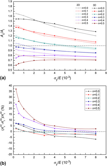
The actual projected contact area A c is normalized with the ideal value A i at the same indentation depth. Hence, the ratio of A c/A i is independent of the indentation depth since the conical indentation and Berkovich indentation are self-similar. The ratio A c/A i is larger than unity for pile-up materials and smaller than unity for sink-in materials. Figure 5(a) shows the values of A c/A i for materials with n = 0.0–0.5 and σ y/E = 0.25–8.0 × 10⁻³ from both the 2D and 3D models. The results show that the contact profile varies largely for different work-hardening rates. The effect of σ y/E on A c/A i also depends on the work-hardening rates. By comparing the values of h c/h and A c/A i, it shows that the h c defined on the mid-plane of facet (plane II) can well represent the contact profile.
(a) Variation of A c/A i with respect to σ y/E and n obtained at a 0.2 μm indentation depth from both the 2D and 3D models. (b) The percentage difference between the projected contact areas obtained from 2D and 3D models for materials with different n and σ y/E.

The difference in the level of pile-up or sink-in produced by different indenters can also be investigated by comparing the value of A c/A i. The relative deviation in the projected contact areas obtained from the 2D and 3D models,  , is shown in Fig. 5(b). For n = 0.0–0.3, the deviations in A c/A i between the conical indentation and Berkovich indentation are in the range of ±5%; the conical indentation produces slightly less pile-up than the Berkovich indentation when σ y/E is high and slightly more pile-up when σ y/E is low. For n = 0.4–0.5, the discrepancy in A c/A i between the conical indentation and Berkovich indentation becomes significant, especially for materials with low σ y/E. For example, the deviation in A c/A i exceeds 35% for material with σ y/E = 0.25 × 10⁻³ and n = 0.5. The reason is that the mechanism of the plastic deformation in the conical indentation and Berkovich indentation is dissimilar for materials with these work-hardening rates; the positive correlation shows up at these work-hardening rates in the Berkovich indentation, but not yet in conical indentation. Therefore, it is necessary to use 3D models to represent the Berkovich indentation, especially for materials with high n and low σ y/E.
As A c is determined based on the contact pressure in each element, it is regarded as the true projected contact area in the model. Alternatively, the projected contact area can be estimated from the load–displacement curve through the Oliver–Pharr method,Reference Oliver and Pharr2 denoted as  . The relative error in
 was calculated as
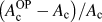 . A negative value of
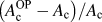 means an underestimation of the projected contact area, which is corresponding to the pile-up phenomenon; and a positive
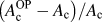 indicates an overestimation of the projected contact area, which is corresponding to the sink-in phenomenon.
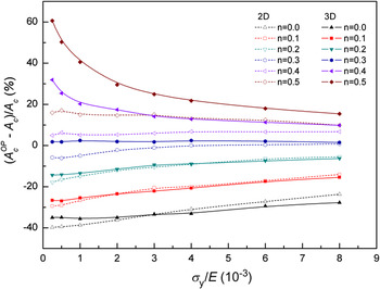
Figure 6 shows the variation in 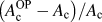 with respect to σ y/E and n from both the 2D and 3D models. The projected contact area is underestimated for materials with low work-hardening rates and overestimated for those with high work-hardening rates. Note that the errors are minimal when n = 0.3 compared to other work-hardening rates. This suggests that the Oliver–Pharr method gives good results when materials have a small level of sink-in. For n < 0.3, A c is generally underestimated, and the lower the n the larger the errors. For n ≥ 0.4, A c is overestimated, and the error increases with n. Thus, the work-hardening rate is the main factor influencing the accuracy of the Oliver–Pharr method. In the 3D model, it is noticed that the errors in
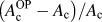 become significant for material with high n and low σ y/E, i.e., 60% for the material with σ y/E = 0.25 × 10⁻³ and n = 0.5. As discussed before, it is known that the sink-in is enhanced with low σ y/E when n ≥ 0.4 in the 3D model. As a result, the relative error
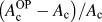 is exaggerated due to the reduction in A c for materials with high n and low σ y/E. Hence, extra attention is required when applying the Oliver–Pharr method to materials with high n and low σ y/E.
Variation of 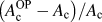 with respect to σ y/E and n obtained at 0.2 μm indentation depth from both 2D and 3D models.

IV. CONCLUSIONS
In the present study, a 3D finite element model has been developed to simulate the nanoindentation of elastoplastic materials with a perfect Berkovich indenter. The contact profile has been studied for materials with σ y/E and n varying from 0.25 × 10⁻³ to 8.0 × 10⁻³ and 0.0 to 0.5, respectively. Compared to the 2D axisymmetric model, the 3D model is more representative of the Berkovich indentation with respect to the geometry of the indenter and the plastic deformations incurred. It has been shown that a low σ y/E not only enhances pile-up in materials with a low work-hardening rate but also enhances sink-in for materials with a high work-hardening rate. The plastic deformation in the indentation region is found to be lateral-flow dominated at low work-hardening rates and normal-flow dominated at high work-hardening rates. Since the 70.3° cone is not equivalent to a Berkovich indenter in terms of plastic deformation, the transition from the negative correlation to the positive correlation is captured at different work-hardening rates in 2D and 3D models. The errors in the projected contact area calculated by the Oliver–Pharr method can be quite significant for materials with high n and low σ y/E. Therefore, accounting for the effects of the work-hardening behavior is essential to correct the errors in the calculation of the projected contact area caused by the pile-up or sink-in.
ACKNOWLEDGMENTS
The authors acknowledge the financial support from the Australian Research Council (ARC) Australian Laureate Fellowship for P.D. Hodgson. J. Wang is grateful to the financial support from Deakin University through the Deakin University International Research Scholarship.