1. INTRODUCTION
Queues with the processor sharing (PS) service discipline became popular by the work of Kleinrock [16,17,18] and were originally proposed as an idealization of time-sharing (queuing) systems. The recent rise of interest in PS queues is related to their application in the performance analysis of bandwidth-sharing protocols in computer communication networks (see, e.g., Núñez-Queija [20] and Roberts [24]).
Several PS studies have focused on the analysis of the tail of the sojourn time distribution in a case when the service time distribution is heavy-tailed. The asymptotic tail behavior of the sojourn time in the M/G/1 PS queue with a regularly varying service time distribution was derived by Zwart and Boxma in [29] and later generalized by Núñez-Queija in [20] for the case of distributions with intermediately regularly varying tails. They established the following asymptotic relationship between the distributions of the sojourn time V and the customer service time B (with ρ denoting the traffic load):

as x → ∞ (for any two real functions f (·) and g(·), f (x) ∼ g(x) as x → ∞ denotes that f (x)/g(x) → 1 as x → ∞). This equivalence is often called a reduced-load approximation. In [13], Jelenković and Momčilović extended the equivalence result to the case when the service time belongs to a class of subexponential distributions with tails heavier than

. The equivalence (1.1) was extended to other types of PS queue in [12] and [6]. Overall, the sojourn time asymptotics are well understood in the heavy-tailed case.
For PS queues with light-tailed service time distributions, only few results are available. The tail asymptotics for the sojourn time of the M/M/1 PS queue are known and are of quite remarkable form:

for positive constants c, α, and γ0. Flatto [11] obtained this asymptotic tail behavior of the waiting time in the M/M/1 random-order-of-service (ROS) queue. Subsequently, Borst, Boxma, Morrison, and Nauñez-Queija [5] showed that the waiting time distribution in the M/M/1 ROS queue, conditioned to be positive, equals the sojourn time distribution in the M/M/1 PS queue. We note that the proof of Flatto is purely analytical, and a probabilistic proof is still lacking.
Using large-deviation techniques, Mandjes and Zwart [19] analyzed sojourn time asymptotics in the GI/GI/1 PS queue. They derived logarithmic asymptotics for a broad class of light-tailed distributions:

Note that in the M/M/1 case, the decay rate γ0 in (1.3) coincides with the exponential decay rate γ0 in expression (1.2).
Apart from the shape of the asymptotics, it is of interest how large sojourn times take place. In a PS queue, three events might contribute to a large sojourn time: (1) a large service time of the tagged customer; (2) a large number of customers present in the system upon arrival of the tagged customer; (3) an unusually large number of arrivals after arrival of the tagged customer. When service times are heavy-tailed, event (1) is responsible for a large sojourn time. In [19] the authors show that for a broad class of light-tailed distributions, event (3) determines the logarithmic asymptotics (1.3). Specifically, V becomes large if the traffic load ρ is increased to one during the sojourn time of the tagged customer. This intuition is valid under two technical conditions that ensure that the service time distribution is not too heavy and not too light. The conditions in [19] are violated for any distribution with bounded support, such as deterministic service times.
This motivated us to take a closer look at the PS queue with deterministic service times. Specifically, we assume that customers arrive according to a Poisson process with rate λ at a single server. The server operates according to the PS discipline; that is, when there are n customers in the system, each is served with rate 1/n. The service time is constant for all customers, denoted by D. Let ρ be the traffic intensity; ρ = λD. We assume that ρ < 1, so that the system reaches steady state. We investigate the asymptotic behavior of the sojourn time tail. Our main result is that the tail behavior of the steady-state sojourn time V is of the form

for some explicit constants α and γ. Observe that the asymptotic form is fundamentally different from the one for exponential service times. Moreover, from our analysis in Section 3, one can infer that the most likely way to cause the event {V > x} not only involves more work feeding into the system between time 0 and time x but also an increased number of customers at time 0; that is, the event {V > x} occurs by a combination of the events (2) and (3) mentioned earlier.
To prove (1.4), we study the sojourn time of a customer by means of branching processes. The branching process representation and decomposition of the sojourn time into a sum of independent random variables (called delay elements), conditioned on the number of customers in the system, was established by Yashkov [27] for the M/G/1 PS queue and later extended by Ott [21]. This approach was also used by Rege and Sengupta [23] for the M/G/1 queue with discriminatory processor sharing and by Núñez-Queija [20] for M/M/1 PS queues with breakdowns. In this article, we make the additional observation that the underlying branching process for the M/D/1 PS queue is a Yule process, which has been treated by Ross [25]. We use this connection to obtain a simplified derivation of the Laplace–Stieltjes transform (LST) of the delay elements associated with V, which also leads to a relatively simple derivation of Ott's result ([21], formula (5.16)) for the LST of V. Since the number of customers in the system has a geometric distribution, we can apply existing theory for tail asymptotics of geometric random sums to obtain the tail behavior of V.
The remainder of the article is organized as follows. In Section 2 we give a closed-form expression for the LSTs of the distributions of the delay elements of the branching process decomposition. The main result is presented and proven in Section 3. In addition, the asymptotic behavior under heavy traffic is considered. It is shown that the limits with respect to time and traffic load are interchangeable. In the last section we present results from numerical experiments. We compute values of P(V > x) using transform inversion and compare them with values predicted by (1.4). These experiments demonstrate a remarkable accuracy of the obtained approximation (1.4).
2. LAPLACE–STIELTJES TRANSFORM OF THE SOJOURN TIME DISTRIBUTION
In this section we derive the sojourn time LST in the M/D/1 PS queue. In fact, the explicit formula for the LST of V is well known. It was derived by Ott [21] as a special case of M/G/1/PS:

In this section we will give a new simplified proof of this formula using existing results for Yule processes. The first step in our proof is to represent the sojourn time as a function of a branching process. By conditioning on the number of customers in the system upon the arrival of the tagged customer, we will decompose its sojourn time into a number of independent random variables, called delay elements (see [27]). In Section 3 we also use some intermediate results provided by this decomposition in the derivation of the tail asymptotics. Thus, our main focus in this section is on the LST of the delay elements.
To perform a branching process decomposition, we consider the process on a transformed timescale. The time-change method is widely used in the analysis of PS queues (cf. [20,27]). Throughout the article, we perform all investigations depending on the amount of service t attained by the tagged customer, t ∈ [0,D], and not the actual timescale. Moreover, we introduce the process X(t) as the number of customers (including the tagged customer) at the server at the epoch when an amount of service t is received by the tagged customer. We study the sojourn time of the customer in terms of the process X(t). A very useful observation is that on the time interval until the first departure (or time interval during which no departures occur), X(t), t ∈ [0,D], can be considered a Yule process. Recall that a Yule process is a pure birth process in which each individual in the population independently gives birth at constant rate λ.
Let us now discuss the time change in more detail. Denote the number of customers in the system (including the tagged customer) at time x by Q(x). The amount of service received by the tagged customer during the time interval [0,x] is

Then the process X(t) introduced in (2.2) can be defined as X(t) = Q(T−1(t)).
Evidently, the sojourn time V0 can be expressed in terms of the process X(t) as

The remainder of this section is organized as follows. First, we consider the situation when the tagged customer enters an empty system. We derive the LST of the sojourn time of this customer. Then we turn to the general case when there are a number of customers in the system upon arrival of the tagged customer. We give a detailed description of the sojourn time decomposition into delay elements and, finally, we prove Ott's formula (2.1).
2.1. Sojourn Time of the First Customer
In this subsection we derive the LST of the sojourn time of the first customer (i.e., the customer that enters an empty system). Notice that in this situation, the above-defined process {X(t),t ∈ [0,D]}, where t is the amount of service received by the first customer, is a Yule process. In our model the births correspond to customer arrivals. Until the service requirement of the first customer is completed, a number of other customers might arrive but none leave the system before that time, since under the PS discipline with constant service requirements, customers depart from the system in order of their arrival.
The next proposition gives the LST of the first customer's sojourn time. From now on we will use variable t as time in the changed timescale.
Proposition 2.1:

Proof: The integral representation (2.3) of V0 can be rewritten as

where (tk,k ≥ 1) are the arrival times of customers that enter the system during the service of the first customer.
Since {X(t), t ≥ 0} is a Yule process, its marginal distribution is known (see, e.g., [25, p.236]). At time t, the population size is geometrically distributed with parameter e−λt:

Furthermore (again see [25]), the conditional joint probability density of the arrival times t1,t2,…, tn, given the number of customers X(t) = n + 1, is given by

where

In order to obtain the expression for the LST of V0, we condition on the number of customers in the system upon departure of the first customer:

where, due to independence of the tk,k = 1,…, n, the conditional expectation is

Computing the inner term of the above product, we get

Hence,

Substituting (2.11) into (2.8) we obtain the LST of the sojourn time,

Rewriting this gives (2.4). █
Remark 2.1: Interestingly, an analog of the above result is given in [15]. The authors considered an M/G/1 queue with any symmetric queuing discipline (processor sharing is a special case). Let B be a generic service time and let D1 be the time until the first departure from the system. Assume that the system is empty at time 0. Then for any positive s,
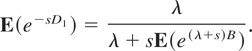
The expression is related to the LST of V0 as

which is a natural result since

, where A1 is the time until the first arrival.
2.2. Sojourn Time of an Arbitrary Customer
Let us now turn to the derivation of the LST of the sojourn time of a customer that enters the system and sees a number of customers already in service upon its arrival. Denote its sojourn time by V. Suppose that the number of customers in the system upon its arrival is Q. As earlier X(t), t ∈ [0,D], is the number of customers at the epoch when an amount of service t is received by the tagged customer. Then X(0) = Q and X(0+) = Q + 1.
Proof of (2.1): Conditioning on the number of customers in the system upon the arrival of the tagged customer, we can write the LST as

Due to the PASTA property, the probability that the tagged customer sees n other customers upon arrival is P(Q = n) = (1 − ρ)ρn, where ρ is the traffic intensity.
Now we use a special decomposition of the sojourn time given the number of customers in the system upon arrival, first established by Yashkov [27]. Every customer in the system at t = 0 is called a “progenitor” and the new arrivals occurring after t = 0 are assumed to be “descendants” of these progenitors. The tagged customer is considered a progenitor. If n customers are present in the system, then each new arrival is declared with probability 1/n as a descendant of any of these progenitors. Each branching process is formed by one progenitor and its descendants (for more detail, see [27]). Therefore, the sojourn time is decomposed into a sum of independent delay elements associated with n + 1 progenitors:

where Ci, i = 1,2,…, n, are independent and identically distributed (i.i.d.) random variables equal to the sum of attained service of the ith progenitor (customer) and its direct descendants for the time interval during which the tagged customer will be served until completion (sum of all lifetimes up to epoch D). Let Ri be the remaining service requirement of the ith progenitor at the moment of the tagged arrival. Ri is uniformly distributed on the interval [0,D].
Using representation (2.15), the conditional expectation in (2.14) simplifies to

Let us now derive the transform of the random variable Ci. Conditioning on Ri, we get

Given Ri = t, we can express the conditional expectation E(e−sCi|Ri = t) as in Section 2.1. However, in this situation we must distinguish between the intervals [0,t] and [t,D]. Since no departures happen before t, on the interval [0,t] we can apply ordinary Yule process properties as for V0. On the interval [t,D], we represent the number of customers in the system as a Yule process as well: The Yule process Y(s), s ∈ [0,D − t], that starts from the number of customers at the moment s = 0: Y(0) = X(t) − 1.
Rewriting the conditional expectation

and using the memoryless property and (2.5), we have

Applying (2.10) with D replaced by t, we can simplify this expression to obtain

For the expectation term on the right-hand side, we perform a computation using the Yule process that starts from m individuals [25]. If the population starts from i individuals, the population size at epoch t is the sum of i i.i.d. geometric random variables with parameter e−λt. Hence, the population size at epoch t has a negative binomial distribution with parameters i and e−λt. As earlier, the distribution of arrival times tk is defined by (2.6). Using these facts, we obtain

Thus, substituting this into the expression for E(e−sCi|Ri = t), we get

and

Substituting (2.4) and (2.20) into (2.14), we obtain the sojourn time transform

which coincides with Ott's formula (2.1). █
In the next section, we will use the equalities (2.19) and (2.20).
3. TAIL BEHAVIOR OF THE SOJOURN TIME
In this section we investigate the behavior of P(V > x) as x → ∞. The following theorem is our main result.
Theorem 3.1: As x → ∞,

where γ is the real solution of

and

Our derivation is based on the results obtained in the previous section. In particular, we will need the moment generating functions of the decomposition random variables V0 and Ci, appearing in the representation (2.15) of V:


This section is organized as follows. In Section 3.1 we analyze the singularities of the above moment generating functions with respect to s. This enables us to prove Theorem 3.1 with a version of the Cramér–Lundberg theorem for geometric random sums. The proof is given in Section 3.2. In Section 3.3 we show some implications of the obtained result.
3.1. Singularities of the Delay Element LSTs
Let us consider singularities of the moment generating function E(esV0). It is enough to consider only real values of s, since

Let us rewrite the denominator of E(esV0) as a function f (s) = λ − se(λ−s)D. Obviously, singularities of the moment generating function might be only at zeros of the denominator. The trivial zero of f (s) is s = λ. However, this is a removable singularity of E(esV0): Using L'Hospital, we obtain that

However, there exists another zero of the function f (s). The derivative of f (s) is determined as f′(s) = (Ds − 1)e(λ−s)D and f′(s) = 0 at s = 1/D. Furthermore, f (0) = λ, f (∞) = λ, f (λ) = 0, and, by stability, λ < 1/D. Since f′(s) < 0 for s < 1/D and f′(s) > 0 for s > 1/D, we can conclude that there is a unique point γ0 > 1/D > λ such that f (γ0) = 0. An important issue is that this point is a pole of the moment generating function: E(eγ0V0) = ∞.
To analyze the behavior of E(esCi), let us consider the conditional moment generating function E(esCi|Ri = t), t ∈ [0,D]:

We already know the zeros of the denominator: λ and γ0. Similarly, λ is a removable singularity since

However, we still have to check if E(esCi|Ri = t) has a singularity when s = γ0. For this purpose we consider the numerator as a separate function: ft(s) = λ − se(λ−s)(D−t). As a function of the parameter t, the numerator ft(s) increases for values s < λ and decreases for s > λ. Since f0(γ0) ≡ f (γ0) = 0 and γ0 > λ, it follows that ft(γ0) is strictly negative for any t > 0. Hence, γ0 is a pole: E(eγ0 Ci|Ri = t) = ∞.
Summarizing this subsection, we have
Proposition 3.1: There exists a unique value γ0 > λ that satisfies the equation

and that is an abscissa of convergence of both E(esV0) and E(esCi|Ri = t), ∀t ∈ [0,D], and consequently, of E(esCi).
We are now ready to give a proof of Theorem 3.1.
3.2. Proof of Theorem 3.1
For convenience, denote the sum

in (2.15) by V1. As earlier, Q is the number of customers in the system upon arrival. The probability distribution of V1 can be written as

where F denotes the distribution of Ci, and Fn(x) is the n-fold convolution of F with itself. The random variable V1 is called a geometric random sum and such random sums are used in many applied probability settings. In particular, it is well known (see [3,10,14]) that P(V1 > x) is asymptotically (x → ∞) equivalent to the exponential function

if there exists a γ > 0 (the Cramér exponent) such that it satisfies the Cramér condition

Note that the Cramér condition (3.12) can be presented as follows:

Since the function E(esCi) monotonically increases from 1 to ∞ on the interval [0,γ0) (by Proposition 3.1), for any nonzero value of ρ there exists a unique real solution γ of the preceding equation, γ < γ0.
Substituting (2.20) for E(esCi) into (3.13), we get (cf. (3.2))

Thus, we have proved the following.
Proposition 3.2: There exists a unique solution γ of (3.2), γ < γ0, that is an abscissa of convergence of E(esV1).
To determine the coefficient kC, we apply the following theorem.
Theorem 3.2 ([2,14]): Let the Cramér condition (3.12) hold. If

, and F is nonlattice, then the asymptotic relation (3.11) holds with

Since the moment generating function E(esCi) is differentiable in point s = γ, γ < γ0, it follows that g < ∞ and we can determine the coefficient kC and asymptotics for P(V1 > x).
Determining the derivative of the moment generating function, performing some simplification, and substituting condition (3.13), we obtain

Hence, by Theorem 3.2, the coefficient kC is

Finally, F is nonlattice, since P(Ci = Ri) > 0, and Ri has a density.
Summarizing the above, we obtain the asymptotic behavior of the random variable V1.
Proposition 3.3: Let γ be the solution of (3.2). Then

Knowing the LST of the first customer's sojourn time V0 and the asymptotic tail behavior of V1, we can derive an expression for the tail behavior of the sojourn time V.
Since V1 has an asymptotically exponential tail and E(e(γ+ε)V0) < ∞ for any 0 < ε < γ0 − γ, we can apply Breiman's theorem to eV0 and eV1 (see [7]):

The above proposition and substitution of γ in (2.4) imply (3.1).
Remark 3.1: An interesting issue, raised in Section 1, is how the number of customers in the system affects a large sojourn time. Mandjes and Zwart [19] have shown that in PS queues with, for example, phase-type service times, the initial number of customers is of o(x) when V > x. In this remark, we show that this picture drastically changes when service times are deterministic.
The proof of Theorem 3.1 indicates that the realizations of the Ci's in the representation

are sampled from the exponentially tilted density eγx dP(Ci ≤ x)/E(eγCi). Under this density, the expected value of the Ci is

Thus, in order for V to be of size x, N should be around x/c(γ).
Remark 3.2: When s = λ, the denominator and the numerator of (3.2) are both equal to zero. Using L'Hospital, we get

Solving the equation

we obtain that, for

, (3.2) has a solution γ = λ.
Since the asymptotic constant α in (3.1) has a removable singularity at this value, the tail behavior of V becomes

3.3. Implications of Theorem 3.1
In this subsection we treat a number of implications of our main result. First, we take a look at the relationship between the decay rate in the M/D/1 PS queue and decay rates in queues with first in–first out (FIFO) and last in–first out (LIFO) disciplines. Second, we consider the behavior of the decay rate γ in heavy traffic.
3.3.1. Other service disciplines.
First we consider the FIFO service discipline. Due to a result of Ramanan and Stolyar [22] it follows that FIFO is optimal among all single-class work-conserving disciplines; that is, it maximizes the decay rate. We can easily show that γFIFO > γPS. Recall (4, Thm. XIII.5.2) that γFIFO is a solution of the equation ρE(esBres) = 1, where Bres is the remaining service time, which is Ri in the notation of Section 2. Using (3.13) and the definition of Ci, we get

The decay rate inequality γFIFO > γPS follows from monotonicity of the moment generating functions on the interval [0,γ0].
The strict inequality was also shown in [19] for the GI/G/1 PS queue for a class of light-tailed service time distributions excluding deterministic service time. Moreover, in [19] it was shown that in the M/D/1 queue, the decay rate under the LIFO discipline does not exceed the decay rate in the PS case: γLIFO < γPS.
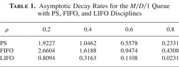
Table 1 shows decay rates for the M/D/1 queue with PS, FIFO, and LIFO disciplines. For convenience, we take D = 1. A result in Cox and Smith [8] implies that in this case, γLIFO = −log ρ − (1 − ρ). The small value of γLIFO for ρ = 0.8 is related to the fact that γLIFO = O((1 − ρ)2) as ρ → 1, opposed to γFIFO = O((1 − ρ)). In the next subsection we show that in heavy traffic, γPS behaves like γFIFO.
Asymptotic Decay Rates for the M/D/1 Queue with PS, FIFO, and LIFO Disciplines

3.3.2. Heavy Traffic.
Let us now study the sojourn time of a customer under heavy traffic (i.e., when the traffic intensity ρ → 1).
Proposition 3.4: Let γ and α be defined as in Theorem 3.1. Then as ρ → 1, the decay rate γ ∼ λ(1 − ρ) and the coefficient α → 1.
Proof: Obviously, when the traffic intensity ρ → 1, the decay rate γ is converging to zero (see (3.13)). Let us study the behavior of γ near zero in more detail. We expand the left-hand side of (3.13) into a two-term Taylor series: E(eγCi) = E(1 + γCi + O(γ2)). The second-order term is O(γ2) uniformly in ρ, since the second moment E(Ci2) is finite if ρ = 1. The smoothness of the moment generating function E(eγCi) near zero implies that all moments of Ci are finite. To calculate the first moment ECi, let us take the derivative of the moment generating function at zero: ECi = (2 − ρ)/ρλ → 1/λ, and due to ρE(eγCi) = ρ + γECi + O(γ2) = 1, we get that

and γ ∼ λ(1 − ρ).
Substitution of the expression for γ into (3.3) gives the behavior of the asymptotic constant α:

█
Remark 3.3: The above heavy-traffic behavior is related to a result of Yashkov in [28]. He derived a heavy-traffic limit result for the sojourn time in the M/G/1 PS queue conditioned on the service requirement. Replacing s in (2.1) by (1 − ρ)s and taking the limit when ρ → 1, we have

Since the limiting value is the LST of the exponential distribution with parameter λ, we obtain the heavy-traffic approximation

Hence, summarizing Proposition 3.4 and Remark 3.3,

This suggests that the asymptotics given in Theorem 3.1 provide a good approximation of the sojourn time tail behavior if ρ is close to one. The results in the next section confirm this.
4. NUMERICAL EXPERIMENTS
In this section we present some numerical results. In particular, we compare the behavior of the sojourn time tail computed numerically from Ott's formula (2.1) with the asymptotics we have obtained. In Ott's formula the sojourn time distribution is expressed in terms of its LST.
The inversion of the Laplace transform was considered to be numerically challenging for a long time. However, currently there are a number of reliable and effective inversion methods that allow for computing probabilities and other quantities without any complication. In our study we will compute the sojourn time distribution using the inversion algorithm of Den Iseger [9] and will perform a cross-check with the algorithm proposed by Abate and Whitt [2]. Both methods are known to perform with high accuracy and produced similar results. Since the sojourn time distribution has a jump at point D, we will apply the modified Den Iseger algorithm for functions with discontinuities.
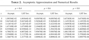
Table 2 shows computational results for various arrival rates and service requirements normalized to D = 1. For each value of ρ, the first column shows, for different values of x, the approximation (3.1) for P(V > x) based on the asymptotic expansion. The second column presents the estimates derived with the Den Iseger inversion algorithm.
Asymptotic Approximation and Numerical Results

The result shows a remarkable accuracy of the asymptotic tail approximation. The numbers obtained with LST inversion and the asymptotic formula differ sometimes within 10−16, which is in fact the maximum accuracy of the inversion algorithm. Moreover, the asymptotics perform well even for relatively small values of x. Already for x = 10 the error is of order 10−13. Results with similar accuracy of exponential asymptotics in FIFO queues are presented in work of Abate, Choudhury, and Whitt [1, Table 1].
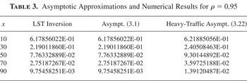
Table 3 presents results for the model with high load, ρ = 0.95. As before, the service requirement D is equal to one. We consider two approximations: the asymptotic approximation from Theorem 3.1 (second column) and the heavy-traffic asymptotics (3.22) (third column). The first column shows the results from the numerical inversion. Remarkably, the heavy-traffic asymptotics perform less accurately than approximation (3.1).
Asymptotic Approximations and Numerical Results for ρ = 0.95

Acknowledgment
This research is partially funded by BRICKS, EURO-NGI, and two NWO grants.