1. Causality of dynamical systems

In the beginning of our topic, in modern times, there was the philosopher and mathematician Gottfried Wilhelm Leibniz (1646–1716). According to Leibniz, nothing happens without cause (nihil fit sine ratione). But only God can recognize all these truths of reason (vérités de raison). Humans only analyze the ‘labyrinth’ of causal chains in a limited way (e.g. by mathematical methods with the calculus invented by Leibniz). The rest remains contingent and random (vérités de fait). Therefore, Leibniz distinguished two kinds of justification: proofs with logical necessity (e.g. in mathematics) and estimations of probability.

Sir Isaac Newton (1642–1727) explained physical effects by mechanical forces as causes. In his ‘Philosophiae naturalis principia mathematica’ (1687), he assumed three axioms as laws of forces (in the modern version):

1. 1. Law of inertia (lex inertiae).

2. 2. F = m a with F force vector, m mass and a acceleration vector.

3. 3. Law of interaction (action = reaction).

A prominent example of Newton’s force is gravity. In analytical mechanics (Leonard Euler, Joseph Louis Lagrange, etc), causality of causes and effects was reduced to differential equations under certain initial conditions and constraints. The search for causes was replaced by the computation of solutions.

At the end of the 18th century, the age of French Enlightenment and classical mechanics, the astronomer and mathematician Pierre-Simon Laplace (1747–1827) assumed the total computability of causal effects in nature if, in the ideal case of a supercomputer (Laplace spirit), all natural laws and initial conditions are well known. Is the Laplace spirit true in all cases? In the theory of dynamical systems, we can distinguish several forms of causality: in the case of weak causality, a cause determines an effect uniquely. In the case of strong causality, causes do not only determine effects uniquely, but similar causes effectively determine similar effects by a computable map. Mathematically, causality of dynamical systems is modeled by (deterministic) differential equations. In the case of deterministic chaos, any error or tiny change of a cause (initial condition) can lead to exponentially expanding trajectories of effects (butterfly effect). Thus, strong causality is violated, but not weak causality.

Typical reasons of deterministic chaos are the many-body problems. In the case of a two-body problem, an element A is the cause of an effect on an element B. If causes and effects are similar, respectively proportional (in the sense of strong causality), then we get a linear relationship represented by a linear equation which, at least in principle, can be solved. Thus, the spirit of Laplace is confirmed for linear problems. However, in the case of many-body problems, more than two elements of a dynamical system interact in complex causal feedback loops simultaneously.

Feedback causal loops lead to nonlinear dynamics, which can be illustrated by the logistic curve of populations. The positive causal loop of the S-shaped logistic curve starts with exponential growth: an increasing number of animals in the population reproduces an increasing number of children. As a population approaches its carrying capacity, resources per capita diminish, thereby reducing the fractional net increase rate until there are just enough resources per capita to balance births and deaths, at which point the net increase rate is zero and the population reaches equilibrium. Mathematically, the dynamics of growth is represented by a nonlinear equation depending on the growth rate as a control parameter. The corresponding population curve is an example of a time series approaching a fixed point attractor, which does not change in the long run.

In general, times series of data are characterized by different degrees of complexity corresponding to different attractors of dynamical systems.¹ They represent different kinds of causal interaction in complex systems depending on changing control parameters. A population curve in equilibrium means weak growth (low value of the control parameter). In the case of stronger growth, we observe oscillations with periodic and quasi-periodic patterns: the growth of population fluctuates and is no longer optimally adapted to the ecological equilibrium. Finally, at a critical value of growth (control parameter), chaos with completely irregular and non-periodic behavior emerges, sensibly depending on initial data. Deterministic chaos is still an example of weak causality.

Time series of dynamical systems correspond to phase portraits of their state spaces, which provide an extremely important method to analyze causal dynamics. The state of a dynamical system is defined by different components, e.g. location and momentum determining the state of motion of a pendulum. The components of a state are considered coordinates of the state space. Thus, the state of a dynamical system is geometrically represented by a point in its state space defined by the components of the state as coordinates. A fixed point corresponds to the state of equilibrium with a fixed point attractor. If the state of the dynamical system changes in time, a curve is generated in the state space. In the case of periodicity, a closed curve (limit cycle) is generated in the state space because of the repetition of states. In the case of chaos, the trajectory of the state develops in a completely irregular and non-periodic way in a limited region of the state space: the typical shape of a chaos attractor emerges.

2. Causality and probability

Contrary to the completely deterministic world of classical mechanics, modern science mainly assumes probabilistic models of the world. Historically, David Hume (1711–1776), the leading philosopher of Scottish Enlightenment, criticized ontological concepts of causality that cannot be justified by perception and observation: ‘There is not, in any single, particular instance of cause and effect, anything which can suggest the idea of power or necessary connection.’Reference Hume² Hume proclaimed that the relation of causes and effects is only a psychological association of perceptions that are repeated for several times (e.g. flash of lightning and thunder). Thus, causality is only the result of psychological habituation to correlated events. Mathematically, Hume considered probabilistic frequencies and correlations of data and derived conclusions by extrapolations.

According to modern theory of probability, causes can be characterized probabilistically.

An event Y_t′ at time t′ is a cause of an event X_t at time t if and if (iff)

1. (1) X_t is later than Y_{t ′} (t′ < t),

2. (2) probability of Y_{t ′} is larger than zero (P(Y_{t ′}) > 0),

3. (3) probability of X_t under the condition of event Y_{t ′} is larger than the probability of X_t without this condition (P(X_t| Y_{t ′}) > P(X_t)).

An event Y_{t ′} is a direct cause of event X_t at time t iff for no point of time t″ between t′ and t (t′ < t″ < t) an event Z_{t ″} influences the probability of X_t, which means, formally: for P(Y_{t ′}|, Z_{t ″}) > 0 is P(X_t| Z_{t ″}, Y_{t ′}) = P(X_t| Y_{t ′}). Y_{t ′} is called a determinate cause of X_t iff P(X_t| Y_{t ′}) = 1.

Geometrically, a causal network can be represented by a directed graph with nodes for variables, e.g. X and Y of data and directed edges X→Y as causal relations. If no common causes are omitted from a set of variables, the set is causally sufficient. A network is acyclic if there are no connected sequences of arrows in the same direction that enters and exits the same node. A node with no edge directed into it is called exogenous or an independent variable. An example of a causal network is an alarm network for medical emergencies, informing physicians about sequences of medical measures.

In the sense of Hume, statistic data analysis (e.g. log-linear methods, logistic regression methods) often yields information on correlations only, but not on causation. It is historically remarkable that during Hume’s lifetime, the Reverend Thomas Bayes (1702–1761) introduced a new method to compute probabilities of hypotheses under the condition of certain information. Although Bayes was never a university professor, he became a member of the Royal Society and left an ingenious ‘Essay Towards Solving a Problem in the Doctrine of Chances’ with pioneering ideas of a new probabilistic approach. Bayesianism is interesting for causal networks, because they can be characterized by Bayesian probabilities. Causal Bayesian netsReference Pearl³ connect acyclic causal networks with probabilistic data distributions satisfying the Markov assumption: let X be a variable in a causally sufficient set of variables, D the set of all variables that are direct causes of X, and Y any set of variables that are no direct or indirect effect of X. Then X is independent (in probability) of Y conditional on D (abbreviation: ).

A consequence of the Markov condition is that any joint probability of data in a causally sufficient set can be factored into a product of conditional probabilities. Examples:

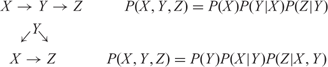
If the causal structure and the probability distribution are known, the probability of any value of a represented variable upon a wide class of interventions forcing specified values on other variables can be calculated from the product of probabilities. For example, a given causal network of genotype (G), smoking (S) and lung cancer (L) provides the joint probability P(S,L,G) = P(L|G,S)P(G)P(S|G):

If not all of the probabilities are known, the theory of interventions on causal Bayesian nets shows what interventions are necessary to find them. The Bayesian net specifies the joint distributions of the variables as a product of conditional probability distribution. Therefore, the conditional probability of any variable can be computed from specifications of the values of any other set of variables. Thus, in the case of Bayesian nets, appropriate interventions and predictions are computable.

However, the question arises, how can we discover the underlying causal networks from probabilistic distributions of data? Distinct causal structures imply distinct-independence and conditional-independence facts. These differences can be exploited in discovery procedures of causal networks. Consider the following example: for three variables, there are 25 distinct acyclic graphs in 11 distinct (Markov) equivalence classes implying the same independencies and conditional independencies. means that X is independent of Z conditional on Y:Reference Glymour⁴

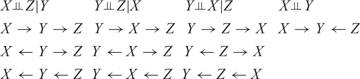
The faithfulness condition assumes that all independencies and conditional independencies are due to the causal structure alone. In this case, if the only independence relation is and if there is no observed common cause of observed variables, then the causal relation is one of the second column. If neither Y nor Z cause X, then the causal relation Y←X→Z is uniquely determined.

The complexity of data and the underlying causal structure are too great for brain-aided humans to process reliable. A simple calculation illustrates the exploding number of possible causal networks with an increasing number of variables. For each pair of variables X and Y, there are four possible kinds of causal networks:

1. 1. X→Y, non X←Y

2. 2. Y→X, non X→Y

3. 3. X→Y, Y→X

4. 4. non X→Y, non Y→X

In general, the number of possible causal models of n variables is 4 raised to the power of the number of pairs variables (e.g. for three variables, 4³; for four variables, 4⁶; for five, 4¹⁰; for six variables, 4¹⁵; for 12 variables, 4⁶⁶ possible causal models). We need computational algorithms that will extract all of the information about causal structures that can be obtained from independencies, conditional independencies, constraints, and the background information (e.g. search strategies of artificial intelligence, machine learning, neuronal networks).Reference Glymour, Scheines, Spirtes and Kelly⁵

3. Causality of natural systems

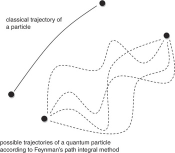
In the previous section, we distinguished an epistemic view of probabilistic data distributions of measurements and an ontological view of underlying causal networks with causes and effects. In the case of Bayesian networks, data distributions and underlying causal networks are connected and allow us to draw conclusions from one and the other. But this is only true in classical physics. In the quantum world, classical states (e.g. location and momentum of a ball) with uniquely determined trajectories are replaced by quantum states with probability distributions of possible trajectories of quantum systems (Figure 1). According to Heisenberg’s principle of uncertainty, the classical assumption of uniquely determined trajectories must be refuted, because location and momentum of, for example, an elementary particle cannot be measured independently with arbitrary exactness. Nevertheless, the development of quantum states is causally uniquely determined by a time-depending differential equation (e.g. Schrödinger’s equation).

Figure 1

Classical trajectory and distribution of possible quantum trajectories.

For Einstein, probabilistic distributions are only epistemic approximations. He strictly believed in the underlying causal networks as ontological fundamentals, mathematically modeled by deterministic differential equations and representing the true reality. ‘God does not throw dice’, he argued in a popular (abbreviated) quotation.Reference Calaprice⁶ In 1935, there was an engaged debate between Einstein and Niels Bohr on causality and a new relationship in the quantum world, which Erwin Schrödinger called ‘entanglement’. In classical physics, two separated objects can be determined completely and independently. This assumption is called ‘locality’. In quantum physics, there are ‘entangled’ states of quantum systems at different locations with a correlated change of quantum states, but without causal (local) interaction (non-locality).

Einstein suggested an experiment to decide between non-locality and local causality.Reference Einstein, Podolsky and Rosen⁷ In a modern version, pairs of photons emitted in opposite directions from a source are prepared in an entangled state.Reference Audretsch and Mainzer⁸ The polarizations of single photons are undetermined, but mutually vertically correlated. After leaving the source, there are no causal interactions of photons. Measuring the horizontal, respectively vertical, polarization of photon 1 determinates the opposite polarization of photon 2 instantaneously. According to Einstein’s principle of locality, the polarization of photon 2 must be determined before its measurement, because there was no causal interaction during the emission process. According to quantum physics, the polarization of photon 2 was determined by measurement of photon 1 because of their entangled (correlated) state of non-locality. Einstein was falsified, because John Bell’s predictions of a local theory (Bell’s inequalities) – i.e. the assumption of determinate causes of quantum effects independent of measurement – were falsified.

In the macroscopic world, causal processes are obviously connected with an observable direction of development. In thermodynamics, the direction of a causal process depends on the entropy S of a physical system during time dt. The change dS of entropy S consists of the change d_eS of the entropy in the environment and the change d_iS of the intrinsic entropy in the system itself, i.e. dS = d_eS + d_iS. For isolated systems with d_eS = 0, the second law of thermodynamics requires d_iS ⩾ 0 with increasing entropy for irreversible thermal processes (d_iS > 0) and d_iS = 0 for reversible processes in the case of thermal equilibrium. Thus, according to the second law, entropy in an isolated system increases until a state of equilibrium is reached, but a spontaneous decrease was never observed. For example, a glass of water falls to the ground, splits up into several particles, energy diffuses and entropy increases. The development back, with the spontaneous reconfiguration of the glass from the particles and diffused energy, was never observed.

For Ludwig Boltzmann, entropy S is a measure of the probable distribution of microstates of elements (e.g. molecules of a gas) of a system, generating a macrostate (e.g. temperature of a gas). Boltzmann’s explanation of macrostates by statistical distributions of microstates is expressed in his famous formula S = k _B ln W with k _B Boltzmann’s constant and W number of probable distributions of microstates. According to the second law, causal change in an isolated system leads with high probability from order to disorder with increasing entropy. In our example, the splitting glass and energy diffusion illustrates the increasing disorder.

The causal arrow of thermodynamics is connected with the causal direction of cosmic expansion. In our current cosmic models, the cosmic process of expansion started with an initial quantum state of symmetry in the sense of a unified theory, followed by symmetry breaking and generating elementary particles, leading to diversity and complexity of galactic structures. High symmetry and order means a distinguished state of less entropy and, following Boltzmann’s formula, less probability. The second law demands a probabilistic transition from order with less entropy to disorder with high entropy, e.g. thermal radiation.

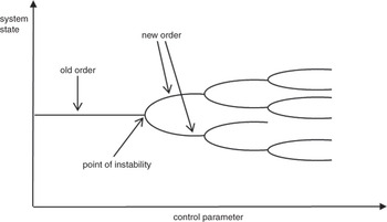
But what is the cause of emerging cosmic structures? In the expanding universe of globally increasing entropy, local islands of new order and less entropy merge like, for example, stars, planets, and life with increasing diversity and complexity. The local emergence of order is made possible by phase transitions (‘symmetry breaking’) of equilibrium states in open systems interacting with their environment. In the theory of complex dynamical systems,Reference Mainzer⁹ the causal order of phase transitions is illustrated by a bifurcation tree (Figure 2). Old order (e.g. patterns of a fluid) becomes unstable near to a point of instability (e.g. critical value of a control parameter), random fluctuations emerge and new order (e.g. vortices in a stream) are selected, followed by a cascade of patterns with increasing complexity, depending on increasing values of a control parameter (e.g. velocity of a stream).

Figure 2

Causal order of phase transitions in a bifurcation tree.

The causal order of phase transitions is not only confirmed in physics, but also in the life sciences. On Earth, the energy of the sun is transformed into different kinds of energy (e.g. light energy assimilation CO₂→sugar, CO₂ + H₂O, chemical, sound, mechanical, electrical, light energy). These forms of energy are ordered in causal cycles driving on the evolution life.

The growth of an organism is causally determined by its genetic information. The genome project was a reductionist research program to explain the emergence of an organism by the genetic sequences of DNA. But it fails to explain the diversity and complexity of cells and organisms. An old truth of complex systems is obvious: the whole is more than the sum of its parts. Therefore, the goal of modern systems biology is to develop models describing and predicting cellular dynamics at the whole-system level.Reference Kaneko¹⁰

However, the paradigm shift from molecular reductionism to the whole-system level of cells, organs and organisms needs an immense increase of computational capacity, in order to reconstruct causal metabolic and regulatory networks at different molecular levels and to understand complex functions of regulation, control, adaption, and evolution. At the sub-cellular level, the nodes of these networks represent genes or proteins causally interacting via connecting edges. Their connections are not uniformly distributed, but form different clusters of high connectivity with specific tasks of regulation, control or metabolism. It is a remarkable insight of complexity research that these causal networks have universal properties (e.g. scale-invariance, power laws), which are not only true in life sciences, but also in technical networks (e.g. the internet).

An important structural characteristic of causal metabolic networks and many other complex networks is the power law degree distribution. Most of the nodes in the network have a low connection degree (which means a low number of connections), whereas a few nodes have a very high connection degree. The high-degree nodes dominate the network structure and are called hubs of the network. Most of the nodes are causally connected through the hubs by a relatively short path. The average path length of causal connection between hubs is insensitive to the network scale. Therefore, this type of causal network is called a scale-free network. The scale-free property makes the network robust against random error (e.g. by mutations) because most errors on the less connected nodes do not affect the network connectivity very much. Therefore, such a robust causal structure may be the result of a long revolutionary selection process. Nevertheless, there are structural differences between the metabolic causal networks of different organisms.

The scale-free property only reflects one aspect of a complex causal network. Actually it only shows the local connectivity of a network, but does not tell anything about the global network structure. For example, there are fully connected networks and other ones consisting of several disconnected sub-graphs, which both have power-law degree distribution. Actually, metabolic networks are far from fully connected networks. In a cell, there often exist several fully connected sub-networks in which all metabolites can be converted to each other. These fully connected sub-networks are called strong components of a network. In graph theory, a strong component of a causal network is defined as a subset of nodes such that for any pair of nodes in the subset there is a path of causal connection from one node to the other. The size distribution of the strong components in the metabolic causal network of the bacterium E.coli is remarkable. It can be seen that the largest component is much larger than other components, and thus is called the giant strong component.

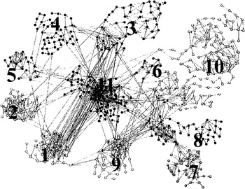
This causal structure of metabolism was empirically found in all other organisms. It is also true in the web page graph in which web pages represent nodes and hyperlinks represent links. This discovery in different types of causal networks implies that it is a common structure in large-scale networks. Causal networks with strong components and giant strong components may be important for the complex systems to be robust and evolvable under variable and undetermined environmental conditions. In large-scale metabolic networks such that of E.coli, it is a goal of systems biology to decompose them into relatively independent functional subsets or modules for further biological functional analysis. For network decomposition, reaction graphs are more convenient than metabolic graphs. In a metabolic graph, the nodes are metabolites and the links are the causal reactions. But in a reaction graph, the nodes are the causal reactions and two reactions are linked if a metabolite is the substrate of one reaction and the product of another reaction. This allowed us to classify reactions into different modules. The reaction graphs also show the power law degree distribution with strong components. In Figure 3, the metabolic network of E.coli is decomposed in several modules, which are distinguished by different biological functions of metabolism.

Figure 3

Functional modules in the metabolic network of E.coli obtained by causal network decomposition.Reference Ma and Zeng¹¹

One of the goals of systems biology is to develop mathematical models to describe and predict causal interactions at the whole system level. The macroscopic structure of the metabolic network with their scale-free organization, which can only be uncovered by analysis of the network as a whole, indicates important system-level principles governing the causal organization of interacting cellular components, such as enzymes and metabolites. Although these structure properties still merely give a static picture of the metabolic network, they can serve as a blueprint for analyzing the dynamic behavior of the causal networks with information and material flows.

Because of their complexity, causal genetic networks cannot be discovered by brain-assisted scientists alone. Machine learning and high-speed supercomputers are necessary. Machine learning algorithms are powerful tools for identifying causal gene regulatory networks from observational gene expression data. In the following, we introduce dynamic Bayesian networks (DBN). Appropriate DBN-algorithms can infer cyclic feedback loops, strength and direction of regulatory influence. Search heuristics are, for example, genetic algorithms, simulated annealing, or greedy search. In systems biology, true causal genetic systems are simulated, for example, by the program Gene Sim with gene expression data.Reference Yu, Smith, Wang, Hartemink and Jarvis¹²

One of the most promising methods to discover complex genetic networks is the Bayesian network model in which genes are regarded as random variables with linear and nonlinear relationships. We remember that a Bayesian network is a directed acyclic graph for representing causal relationships among random variables by using conditional probabilities. In the gene network estimation based on Bayesian networks, a gene is regarded as a random variable shown as a node. Let X_i (i = 1, 2, …, n) be a discrete random variable and e_ij directed edges from X_i to X_j. X_i is called parent of X_j. The subset Pa(X_j) {X ₁, …, X_n} is the set of parents of X_j. Due to the Markov condition, the random variable X_j only depends on its direct parents Pa(X_j) and is independent of other variables. In this case, the joint probability of all random variables can be decomposed as the product of conditional probabilities .

The conditional probabilities P(X_j | Pa(X_j)) describe the parent–child relationships and can be viewed as an extension of the deterministic models of, for example, Boolean networks. If we know the structure of the causal gene network a priori, we can construct the joint probability function by estimating each conditional probability following the product formula. However, in the gene network estimation, the true causal network is not known and we have to estimate based on the observed data. This problem can be considered a statistical model selection problem.

It is a challenge to find effective methods for estimating causal gene networks from gene expression data using Bayesian networks. A shortcoming of the Bayesian network is that this model cannot construct cyclic networks, whereas a real gene regulation mechanism has cyclic regulations. Cyclic regulations are often very important in the cellular metabolism. The use of dynamic Bayesian networks has been proposed for constructing a gene network with cyclic regulations.Reference Kim, Imoto and Miyano¹³ In the context of the dynamic Bayesian network, we consider time series data corresponding to the states of n genes at time t (t = 1, …, T). The Markov condition is now assumed for the time dependency of the states of the genes. Thus, the time dynamics are causally ordered by X ₁→X ₂→…→X_T.

Under this condition, the joint probability can be decomposed as P(X ₁, …,X_T) = P(X ₁)P(X ₂ | X ₁) … P(X_T | X_{T −1}). The gene regulations can be modeled through the construction of P(X_t | X_{t −1}) for t = 2, …, T. The network structure is assumed to be stable through all time points. The conditional probability P(X_t | X_{t −1}) can also be decomposed into the product of conditional probabilities of each gene for given parents with , where Pa(X_j)_{t −1} is the set of random variables corresponding to the parent genes of the jth gene at time t−1. By combining the two equations, we get the decomposition . From this equation of dynamic Bayesian networks, the detection of nonlinear relationships and the construction of graph selection criteria can be done in the same way as for the Bayesian networks.

However, finding optimal causal networks is an NP-hard problem. Potentially, we need to search the space of directed acyclic graphs of n vertices whose size c_n is approximately

According to this formula, there are roughly 2.34 × 19⁷² networks with 20 vertices and 2.71 × 10¹⁵⁸ for 30 vertices. This complexity does not allow any purely brute force computation even with a supercomputer. Therefore, heuristic approaches have been applied to this search problem, such as greedy algorithms.Reference Heckerman, Geiger and Chickering¹⁵ The greedy algorithm assumes a score function for solutions. It starts from some initial solution and successfully improves the solution by selecting the modification from the space of possible modifications that yields the best score. When no improvement is found, the algorithm terminates with the current best solution. Biologically reasonable locally optimal Bayesian networks of several hundred genes have been reported.

The ontogenetic growth of a cellular organism can be modeled by a causal tree starting with an egg as the initial node, followed by bifurcating branches, which represent cellular specifications and a parallel growth of organs and tissues. Again, a causal tree of bifurcations models the phase transitions of a complex system. Organisms can be characterized by different ontogenetic trees of growth. The phylogenetic tree of life illustrates Darwin’s evolution of species. This causal bifurcation tree is determined by DNA-programs replicating themselves. Again, the bifurcating points of instability are characterized by random fluctuations. In the biological context, they are mutations, as random changes of DNA-codes. Selections are the driving forces in the branches. Rates of mutations measure the causal distances of species.

4. Causality of technical systems

The causality of natural systems often inspires causality of technical systems. In the beginning of modern times, Leonardo da Vinci (1452–1519) was one of the first engineers experimenting with control tasks of causal technical systems (e.g. mechanically driven cars). In engineering sciences, the causal dependence of events must not only be analyzed theoretically, but constructed and controlled, in order to guarantee reliable and desired functions of technical systems. Control is the inverse problem of causality for engineers.

Robotics constructs causal technical systems with great similarity to causal natural systems.Reference Bekey¹⁶ An industrial robot manipulator, or the arms and legs of humanoid robots, consist of rigid links connected by joints. If, for example, two joints are rotated by motors with angles θ, ϕ, it is easy to compute the resulting position change Δx, Δy of a foot or hand as causal effects. This task is called forward kinematics: the knee coordinates x_k = l ₁cos θ, y_k = l ₁sin θ, with l ₁ length of upper leg segment, and foot coordinates x_f = x_k + l ₂cos ϕ, y_f = y_k + l ₂sin ϕ, with l ₂ lower leg segment, yield the (nonlinear) foot equations x_f = l ₁cos θ + l ₂cos ϕ, y_f = l ₁sin θ + l ₂sin ϕ. In general, for joint angles θ_i (i = 1, 2, 3) and position coordinates x_i (i = 1, 2, 3) with vectors θ = (θ ₁, θ ₂, θ ₃)^T and x = (x ₁, x ₂, x ₃)^T, the function x = F(θ) represents the causal effect of position change by rotating joints.

In order to control the position of a multilink system, it is necessary to solve the inverse problem of x = F(θ), which means to compute the rotations of the links θ for a desired goal location x. But the inverse kinematics problem of control may not have a unique solution (e.g. four joint arrangements for a hand position). Therefore, we consider the corresponding invertible rate expression: differentiation of x = F(θ) yields with the Jacobian matrix J(θ) = F′(θ) given by ∂F_j/∂x_k (j,k = 1, 2, 3). The forward kinematics of causality is computable by , the inverse kinematics of control by .

Control as the inverse problem of causality can only be programmed in restricted applications with fewer degrees of freedom. In general, robots cannot be fully programmed with respect to all possible changes in a complex environment. In adaptive household robots, for example, the program learns, from causal interaction with the environment, where to stand when taking a glass out of a cupboard, how to best grab particular kitchen utensils, where to look for particular cutlery, etc. This requires the control system to know the parameters of causal routines and to have models for how the parameters change the behavior.

The sensor data of a robot’s environment are stored in a relational database system. The data in the database together with the causal structure on domain relations imply a joint probability distribution over relations in the activity domain.Reference Thrun, Burgard and Fox¹⁷ This distribution is represented using Markov logic, which allows inferring the conditional probability of logical (first order) statements. In short, the robot learns to estimate and predict situations with a certain degree of probability.

Further technical applications of causal networks are neural networks. Technical neural networks are complex systems of firing and non-firing neurons with topologies like brains. The nodes are neurons with alternative states (‘firing’ or ‘non-firing’), and the causal arrows are synaptic interactions with learning algorithms changing numerical weights, modeling the strength of synaptic connections. A simple robot with diverse sensors of, for example, proximity, light, and collision can generate causal behavior by a self-controlling neural network. In the case of a collision with an external obstacle, neighbored sensors of the robot are activated and the corresponding nodes in the neural network are excited together. With respect to Hebbean learning rules in natural brains, a causal pattern of external representation is generated by reinforced activation of technical neurons.

Neural nets can represent causal behavioral patterns as probability relations corresponding to cognitive stimuli or responses. The net determines a probability distribution over the values of a collection of nodes. The total probability distribution is related to the probability relations between net nodes. For example, consider the following feedforward network with no feedback loop from E to B, C, or D, and no further node influencing both A and B or both A and C. In the second example, all of the causal links between B, C and A are broken and B, C have no direct or indirect causal links with D. Variations in B, C will produce no variation in A. That means in probabilistic terms P(A | B, C) = P(A):Reference Glymour¹⁸

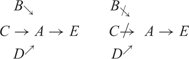
The absence of any causal relation between parts, e.g. lesions of neural connections in the nervous system, is directly reflected in the independence of probabilities of states of those parts. Thus, this is a method to detect lesions in a neural feedforward network. However, in nonlinear recurrent systems, conditional independence does not neatly correspond to lesions of technical networks in robotics or biological brains in medicine.

The largest technical causal network is the World Wide Web (WWW). It has surprising similarities with self-regulating cellular networks in systems biology and neural networks in brain research. Its increasing complexity needs intelligent strategies to detect lesions and to avoid collapse and congestion of data traffic. In general, complex networks can be characterized by clustering and degree distributions. A node i of a network has k_i edges connecting it to k_i other nodes. The total number of edges with the nearest neighbors in a cluster is k_i(k_i−1)/2. The clustering coefficient of node i is the ratio between the number E_i of actually existing edges and the total number, i.e. C_i = 2 E_i/k_i(k_i−1).

The clustering coefficient C of the whole network is the average of all individual C_i. In a random graph, since the edges are distributed randomly, C = p (with probability p). Further, the majority of nodes have nearly the same degree (number) of edges. Therefore, the degree distribution P(k) (probability that any node has k edges) is a Poisson distribution. But most realistic networks in nature and technology have a degree distribution with power-law tails, which means P(k) = k ^−γ without any characteristic scale (scale-free networks).

The World Wide Web is the largest information network, with web pages as nodes and hyperlinks as edges.Reference Mainzer¹⁹ The directed edges are characterized by two degree distributions of outcoming and incoming distributions with power-law tails: P _out(k)∼ and P _in(k)∼. In a sample of 200 million web pages, values of γ _out = 2.72 and γ _in = 2.1 were measured.Reference Réka and Barabási²⁰ Despite the large number of nodes, WWW displays the small-world property (e.g. for a sample of 800 million nodes with a path length of around 19 links). Clustering coefficients need undirected edges. With modifications for bidirectional edges, one gets C = 0.1078, which means orders of magnitude higher than C _rand = 0.00023 corresponding to a random graph of the same size and average degree. Deviations of real networks from the corresponding random graphs C _rand indicate clusters and structures of the underlying causality. Thus, the deviations from the corresponding random graphs are used to discover the technical or biological tasks and functions connected with causal clusters and structures.

In computer technology, it is a challenge to guarantee the causality between input and output of data streams and to avoid causal loops with endless repetitions. Data streams of input and output channels I and O describe the I/O-behavior F of information systems. The I/O-behavior F is deterministic if for each input x there is exactly one output F(x). The timing of inputs and outputs depends on the chosen scaling of time intervals:Reference Réka and Barabási²⁰F is called weakly causal if the output in the tth time interval does not depend on input that is received after time t. F is called strongly causal if the output in the tth time interval does not depend on input that is received after the (t−1)th interval. In this case, F reacts to input received in the (t−1)th interval. Thus, causality between input and output is guaranteed.

In order to compose many components into a complex information system, some of the connecting channels have feedback loops, corresponding to recursive definitions of the data streams. Feeding back all channels corresponds to the fixpoint property x∈F(x). This property characterizes the computations in feedback loops correctly if F is strongly causal. Otherwise, there occur computationally infeasible fixpoints as result of causal loops, where certain output is fed back within the same time interval as corresponding input (‘self-fulfilling prophecies’). Strong causality avoids causal loop information systems.

5. Causality of social and economic systems

Natural and technical causal systems are involved in complex social systems of highly developed societies. Examples are causality networks of spreading disasters, e.g. pandemics, such as SARS or swine flu. Disasters with cascade-like spreading in human society are extreme events, occurring more frequently than expected, according to a normal distribution. Causality networks allow one to estimate their development with time, to give hints about when to take certain actions, to assess the suitability of emergence management, and to anticipate their side effects.

A causality network of spreading disasters consists of n nodes i (1 ⩽ i ⩽ n) as factors or sectors and direct influences M_ij of factor j on i represented by arrows. Directed influences are weighted with, for example, M_ij∈{−3, −3, −1, 0, 1, 2, 3}, where M_ij = ±3 means an extremely positive or negative influence, M_ij = ±2 a strong influence, M_ij = ±1 a weak influence, and M_ij = ±0 a negligible influence. All direct influences are summarized in a matrix M = (M_ij). The expression M^k reflects all influences over k−1 nodes and k causal links (e.g. k = 1: direct influences; k = 2: feedback loops with one intermediate node; k = 3: feedback loops with two intermediate nodes etc). Feedback loops cause indirect effects.

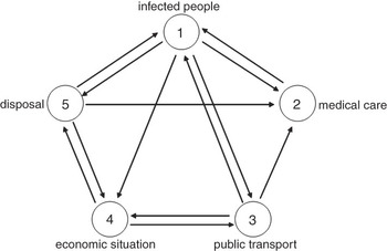
An example is a causality network of epidemics with i,j∈{1, 2, 3, 4, 5}, which is illustrated in a matrix with the following rows, respectively columns:

1. 1: the number of infected people

2. 2: the quality of medical care

3. 3: the public transport

4. 4: the economic situation

5. 5: the disposal of waste

with

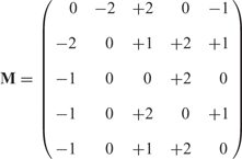
According to Ref. Reference Helbing, Ammoser and Kühnert22, the corresponding causal network can be figured by a regular 5-polygon (Figure 4).

Figure 4

Causal network of spreading disasters and societal effects.Reference Helbing, Ammoser and Kühnert²²

For the purpose of anticipation, we need a dynamical model of the time-dependent spreading of disasters in causality networks with the impact P_i(τ) of factor i at time τ, the rate W_ij at which P_i(τ) spreads to factor j, the damping rate D_i describing the mitigation of the catastrophic impact on factor i by disaster response management, and L_ij = W_ij−δ_ij D_i with Kronecker symbol δ_ij (with 1 for i = j and 0 otherwise).

The dynamics of impacts is related to the Liouville representation of the discrete master equation

The spreading rate W_ij is assumed to be proportional to the strength |M_ij|| of the direct influence of factor j on factor i with W_ij∼c|M_ij||.

In this example, predictions and anticipations of the spreading disaster are possible, because there is a formal solution of the Liouville equation for a time-independent matrix L:

with B(τ) describing the spread of an event in the causality network over time τ and P(0) reflecting the initial impact of a catastrophic event.

Due to the damping rates D_i, we can distinguish the following scenarios:

A detailed picture of potential catastrophic scenarios is computable (e.g. with path integral method: likelihood of specific spread paths of events, approximate appearance time).

The damping is weak. P_i(τ) grows exponentially. Thus, control is lost and the disaster spreads all over the system.

The impact of the disaster decays over time with P_i(τ)→0, as τ→0.

The dynamics depend on the initial impact P(0) and the matrix B(τ).

What can we learn from these insights into the dynamics of causal networks? Under well-defined conditions, scenarios are predictable and computable. At least, we can be well prepared to decide measures of anticipation. However, extreme events are caused by nonlinear effects and characterized by power laws. Small local random events can cause large global effects in the sense of the butterfly effect. A dramatic example was the recent financial and economic crisis.

In general, we do not know all the causal microscopic interactions of economic agents. Therefore, in 1900, the French mathematician Louis BachelierReference Bachelier²³ considered the fluctuations of stock prices as statistical random walk (Brownian motion) before physicists such as Albert Einstein (1905) discovered it in the microscopic motion of small particles in fluids.Reference Einstein²⁴ Bachelier did not only suggest the random walk of price changes, but also considered the effects of investing in options. A breakthrough in 1973 was the famous Black-Scholes formula for calculating the present call option when there is a continuum of possible future stock prices on the basis of a normal (Gaussian) distribution. Every day dealers on the options exchanges still use this formula to make their trades.

Brownian motion is mathematically more manageable than any alternative. But, unfortunately, it is an extremely poor approximation to financial reality.Reference Mainzer²⁵ Since the end of the 1980s, we have observed financial crashes and turbulences deviating significantly from the normal distribution. Investment portfolios collapsed and hedging with options à la Black-Scholes failed. Local failures of single bankers can cause global effects of the whole financial systems because of their nonlinear dynamics. From the viewpoint of dynamical systems, patterns of time series analysis illustrate the failures of traditional financial theory. While a record of Brownian motion changes looks like a kind of ‘grass’ of normal length, a record of actual price changes looks like an irregular alternation of quiet periods and bursts of volatility that stand out from the normal length of the grass. This feature demonstrates the apparent non-stationarity of the underlying rules.

Further on, discontinuities appear as sharp peaks from the normally distributed Gaussian ‘grass’. These peaks are not isolated but bunched together. Cyclic (but not periodic) behavior can be observed. Instability of the sample variance is expressed by a long-tailed distribution of price changes. Last but not least, there is a long-term dependence of data. In the nonlinear and fractal approach of the financial system, randomness can no longer be restricted to the ‘normal’ Gaussian distribution of price changes. Non-Gaussian distributions with Levy- and Pareto-distributions are more appropriate to the wild turbulence of financial markets of today.

From an epistemic point of view, extreme events falsify generally believed hypotheses. Consider the well-known general hypothesis that for all locations and points of time, all ravens are black. The general hypothesis works, until it is falsified by the observation of a single white raven at a certain location at a certain point of time. Extreme events are ‘white ravens’. In particular, reinsurance companies are interested in these rare species and causal models predicting them. But, in nature as well as in society, they can be caused by local random events leading to global effects because of nonlinear dynamics. In the case of white ravens, a mutation may be the cause their occurrence. In economy, local failures of single persons and institutions may initialize global catastrophes in a globalized world with increasing dependence and complexity. Non-Gaussian models help to detect the hints of threatening disasters, in order to be well prepared. These insights are also true with respect to extreme events warning us against climate change.

In economics, the rationality of causal models is bounded by the wild randomness of markets. Human cognitive capabilities are overwhelmed by the complex causal interactions with the nonlinear effects they are forced to manage. Traditional mathematical decision theory assumed the linear causal rationality of economic agents and the complete information of possible causal effects (homo oeconomicus). Herbert Simon, Nobel Prize laureate of economics and one of the leading pioneers of systems science and artificial intelligence, introduced the principle of bounded rationality.Reference Simon²⁶

Bounded rationality is not only given by the limitations of human knowledge, information, and time. It is not only the incompleteness of our knowledge and the simplification of our model. The constraints of short-term memory and of information storage in long-term memory are well-established. In stressful situations, people are overwhelmed by a flood of causal information, which must be filtered under time pressure. People deviate from game-theoretically predicted equilibria. They act neither in the strict sense of the homo oeconomicus nor completely chaotically.

Therefore, we must be cautious with (especially linear) causal models. We must refer to the real features of human information processing and decision making, which is characterized by emotional, subconscious, and kinds of affective and non-rational factors. Even experts and managers often prefer to rely on rules of thumb and heuristics, which are based on intuitive feelings of former experience. Experience shows that human intuition does not only mean lack of information and the failure to make decisions. Our affective behavior and intuitive feeling are parts of our evolutionary heritage that enable us to make decisions when matters of survival are at stake. Therefore, we must know more about the factual causal acting of people, their cognitive and emotional behavior, in order to understand the global trends and dynamics of our complex civilization. Thus, we close with the demand for more interdisciplinary research between humanities, economics, natural and engineering sciences, in order to get more insights into the causal dynamics of complex systems.