1. Introduction
Our concern is with the mechanism by which boundary forcing induces streamwise vortex instabilities in shear flows. We consider the cases when the wavelength is small or of size comparable to the fluid depth. We refer to these as the unbounded and bounded problems respectively. In the unbounded case the instability depends only on the base flow properties near the wall and the appropriate Reynolds number is the friction Reynolds number based on the forcing wavelength. Therefore the forcing wavelength only enters the problem through the Reynolds number. For the bounded case the results depend on the particular flow under consideration and, for definiteness, we take it to be Couette flow. Note that in this work the forcing from the wall is the cause of instability rather than the enabler as in receptivity theory; see for example Ruban (Reference Ruban1984), where boundary layer receptivity is discussed.
Recent work by Hall (Reference Hall2020) and Hall & Ozcakir (Reference Hall and Ozcakir2021), hereafter referred to as H1 and HO, respectively, has shown that a linear theory somewhat similar to vortex–wave interaction theory, VWI for short, describes linear instabilities of flows in wavy-walled pipes and channel. Here, we show that the work of H1 and HO can be readily deduced by linearisation of an extended form of the strongly nonlinear ‘square-vortex VWI’ of Hall & Smith (Reference Hall and Smith1991), hereafter, we refer to the latter paper as HS. The formulation given here greatly simplifies the linear instability theory and is the appropriate starting point to follow the instability into the nonlinear regime. Our asymptotic theory gives results in excellent agreement with related problems investigated numerically and is applied to propagating waves or oblique configurations not tackled previously.
The formulation of VWI theory is due to HS who were concerned with the linear and nonlinear growth of wave-like disturbances in boundary layers. That approach describes how a small wave interacting with itself in its critical layer generates a roll flow which then drives a streak which is neutrally unstable to the wave thereby closing the interaction. The many different forms which the interaction can take are described in HS, but perhaps the most notable one corresponds to the wave being a neutrally stable inviscid Rayleigh instability and it has been shown to describe high Reynolds number exact coherent structures in shear flows; see Hall & Sherwin (Reference Hall and Sherwin2010), Blackburn, Hall & Sherwin (Reference Blackburn, Hall and Sherwin2013), Deguchi & Hall (Reference Deguchi and Hall2014) and Hall (Reference Hall2018). The VWI predictions of the latter authors agree very well with the full numerical computations of for example Wedin & Kerswell (Reference Wedin and Kerswell2004) and Wang, Gibson & Waleffe (Reference Wang, Gibson and Waleffe2007). Related ideas have been used in the context of Langmuir circulations, see for example Phillips (Reference Phillips2002). The fact that we show that VWI is also the mechanism underpinning instability generation by wavy walls or wall transpiration suggests an intriguing interdependence of exact coherent structures and wave-like forcing from for example wall roughness, that relationship is embedded within the extended VWI system we derive here.
We formulate a nonlinear theory describing the interaction of quite arbitrary shear flows with wall forcing. As particular examples we will consider wall transpiration and wall displacements in the form of waves. Our formulation applies to both bounded and unbounded shear flows. For the bounded problem the instability depends on the basic velocity profile everywhere and here we take it to be Couette flow. The interaction equations for the bounded and unbounded problems are almost identical, the only difference being that in one case the disturbance vanishes far from the wall whilst in the other the velocity must satisfy the appropriate boundary conditions at the upper wall. Although we take Couette flow as the prototype bounded flow the approach used is readily applied to other flows. The Reynolds number appears in the same way in the equations of motion for the bounded/unbounded problems. But in the former case it is defined in terms of the fluid depth and the speed of the upper wall whereas in the unbounded case it is the square of the friction Reynolds number.
Motivation for studying the effect of wall undulations comes from the heat transfer community where wavy walls have long been used as an aid to mixing; see for example Kandlikar (Reference Kandlikar2008). Further motivation comes from aerodynamics where there has been a longstanding interest in how wall waviness impacts the transition process; see for example Fage (Reference Fage1943). Numerical investigations by Floryan (Reference Floryan2002, Reference Floryan2007, Reference Floryan2015) in channel flows of periodically varying depth in the streamwise direction showed that streamwise vortex instabilities can be excited and H1 demonstrated that at small amplitudes these can be accurately predicted by high Reynolds number linear stability theory. In pipe flows HO showed that a similar instability is excited and found that pipes corrugated in both the streamwise and azimuthal directions are more stable than those corrugated only in the streamwise direction. Loh & Blackburn (Reference Loh and Blackburn2011) considered only the latter case in their numerical investigations and their results are broadly in agreement with those of HO.
Some previous work has been done on the effect of travelling waves on the stability of Tollmien–Schlichting waves in channel flows. Hall (Reference Hall1978) considered the resonant nonlinear situation when the wave corresponds to the most unstable Tollmien–Schlichting instability of the flow in the absence of the wave. It was shown that in the weakly nonlinear regime the Stuart–Landau equation now has a term independent of the amplitude so that the bifurcation problem is now an imperfect one. Floryan (Reference Floryan2002) considered a similar problem for more general wall shapes in the slightly detuned configuration.
Wall transpiration has often been used as a simplified prototype model to understand the effect of boundary topography on both laminar and turbulent flows; see for example Floryan (Reference Floryan2003), Gómez et al. (Reference Gómez, Blackburn, Rudman, Sharma and McKeon2016), Min et al. (Reference Min, Kang, Speyer and Kim2006) and Quadrio, Floryan & Luchini (Reference Quadrio, Floryan and Luchini2007). Floryan considered the linear instability of Couette flow in the presence of transpiration by first solving the full Navier–Stokes equations for the basic flow and then solving the linearised Navier–Stokes equations. Gómez et al. (Reference Gómez, Blackburn, Rudman, Sharma and McKeon2016) considered the effect of streamwise periodic transpiration on turbulent flows. Where a comparison can be made our results for transpiration agree well with those of Floryan et al. (Reference Floryan2003). In § 2 we describe the extension of what was referred to by HS as the ‘square-vortex VWI problem’ to account for wall forcing. In § 3 we derive the linear stability eigenrelation for travelling wave undulations and transpiration velocities from the nonlinear VWI system. In § 4 we give results for wall undulations and in § 5 results are given for the transpiration problem. Finally in § 6 we draw some conclusions.
2. The interaction equations
Consider a shear flow  $(u^*(y^*), 0, 0)$ with respect to Cartesian coordinates
 $(x^*,y^*,z^*)$, here, a
 $*$ denotes a dimensional variable. We suppose in the first instance that the depth of fluid is large compared with the wavelength
 $b$ of forcing from the boundary. We define the friction velocity
 $u_s=\sqrt {\nu {u^*}' (0) }$ where
 $\nu$ is the kinematic viscosity and use
 $\hat {b}={b}/{2{\rm \pi} }$ as length scale, here the factor
 $2{\rm \pi}$ has been introduced for convenience to simplify the later analysis. If we take a typical velocity to be
 $\hat {b}{u^*}' (0)$, scale time on
 ${1}/{{u^*}'(0)}$, and define the friction Reynolds number
 $R_f={u_s {b}}/{\nu }$ then the dimensionless equations of motion take the form
 \begin{gather} \frac{\textrm{D} {\boldsymbol{\hat{u}}}}{\textrm{D} t} ={-} \boldsymbol{\nabla}{\hat{p}}+\frac{1}{R}\nabla^{2}{\boldsymbol{\hat{u}}}, \end{gather}
 \begin{gather}\boldsymbol{\nabla}\boldsymbol{\cdot} \boldsymbol{\hat{u}} =0, \end{gather}
where  $p$ is the pressure and the Reynolds number
 $R={R_f^2}/{4{\rm \pi} ^2}$ is assumed large. Because we assume the forcing wavelength is small compared with the length scale of the unperturbed flow in the wall-normal direction, and
 $R\gg 1$, the basic state corresponds to
 $\hat {u}=y$ for
 $0< y< \infty$. Thus in the small wavelength limit the flow stimulated by the forcing depends only on the wall shear of the unperturbed flow, and it follows that (2.1) and (2.2) apply to an arbitrary unidirectional shear flow.
If the wall forcing wavelength is comparable to the depth  $d$ of the unperturbed basic flow
 $u^*=\bar {U}\bar {u}({y^*}/{d})$, then (2.1) and (2.2) still apply with
 $R={\bar {U}d}/{\nu }$ and the unperturbed flow then corresponds to
 ${\boldsymbol {\hat {u}}}=(\bar {u},0,0)$. We will refer to the two cases as the unbounded and bounded problems respectively but for definiteness we will take
 $\bar {u}=y$ so that the bounded flow is Couette flow and
 $d$ is the channel depth. The analysis is readily modified when
 $\bar {u}\ne y$ and we shall indicate later the required changes. The upshot then is that we are interested in finding solutions of (2.1) and (2.2) when the unperturbed flow is a uniform shear flow extending to
 $y=1$ or
 $y=\infty$.
Suppose that the wall is defined by
 \begin{equation} y=2\epsilon \cos\left(\alpha x+\beta z -\frac{\omega t}{R^{1/3}}\right), \end{equation}
so that a wave propagates at an angle  $\varTheta =\tan ^{-1}({\alpha }/{\beta })$ to the direction of the basic flow at a speed close to that of fluid in the viscous sublayer of depth
 $R^{-{({1}/{3})}}$ where the flow adjusts to the perturbed wall position. For future reference we note that if
 $h$ is the dimensional amplitude of the wavy wall then for the unbounded problem
 $\epsilon ={{\rm \pi} h}/{b}$ and for the bounded problem, here Couette flow,
 $\epsilon ={h}/{2d}$. Other forms of the wave can be considered and HO considered ’egg-box’ roughness in pipe flow where the undulation is streamwise periodic and modulated in the azimuthal direction. Likewise, if the wall shape contains several harmonics, the theory can be trivially modified in the way indicated in HO. We further assume that
 $\epsilon$, the scaled undulation amplitude, is small compared with the sublayer thickness. For the transpiration problem we suppose the wall remains flat and fluid is injected into the flow such that
 \begin{equation} \hat{v}=2\delta \cos\left(\alpha x +\beta z -\frac{\omega t}{R^{1/3}}\right),\quad y=0, \end{equation}
and  $\delta$ is also assumed small compared with the sublayer thickness. We will refer to the cases with
 $\beta =0, \beta \ne 0$ as the aligned and oblique configurations, respectively.
If we take  $\delta =\epsilon =0$ we recover the ‘square-vortex’ VWI problem introduced by HS. The key point of the square-vortex VWI is that the wave driving the roll part of the roll-streak flow has its critical layer at the wall. Therefore, the roll is sustained near the wall rather than away from the wall as in Hall & Sherwin (Reference Hall and Sherwin2010). The self-sustaining structures described in the latter paper can co-exist with the square-vortex VWI state but interact only weakly with the wall undulations or transpiration. The appropriate scalings are given in HS so we give only the essential details here. For
 $y=O(1)$ we assume the uniform shear flow is deformed into the roll-streak flow
 \begin{equation} {\boldsymbol{\hat{u}}}=\left(u(y,z), \frac{v(y,z)}{R}, \frac{w(y,z)}{R}\right)+\cdots,\quad \hat{p}=\frac{p(y,z)}{R^2}+ \cdots, \end{equation}
where the flow is assumed to be periodic in  $z$ with wavelength
 ${2 {\rm \pi} }/{k}$ and the terms represented by
 $\ldots$ represent higher order corrections to the roll-streak flow and a small wave of size yet to be determined. Note we have made the usual assumption that the roll flow is smaller by a factor of
 $R$ than the streak. For the unbounded problem we require that
 ${\boldsymbol {\hat {u}}}\rightarrow (y,0,0), y\rightarrow \infty$ so that the uniform shear flow is re-established. For the bounded problem
 ${\boldsymbol {\hat {u}}}$ must satisfy the no-slip condition at the upper wall. An important point to note is that the roll-streak flow has spanwise wavenumber
 $k$ whereas the wall forcing has spanwise wavenumber
 $\beta$, the theory we give does not require these to be the same. If the wave is sufficiently small then the roll-streak flow satisfies
 \begin{gather} \frac{\partial v}{\partial y}+\frac{\partial w}{\partial z} =0, \end{gather}
 \begin{gather}\left[\frac {\partial^2}{\partial y^2}+\frac {\partial^2}{\partial z^2}\right]u=v \frac{\partial u}{\partial y}+w\frac{\partial u}{\partial z}, \end{gather}
 \begin{gather}\left[\frac{\partial^2}{\partial y^2}+\frac{\partial^2}{\partial z^2}\right]v= \frac{\partial p}{\partial y}+v\frac{\partial v}{\partial y}+w\frac{\partial v}{\partial z}, \end{gather}
 \begin{gather}\left[\frac{\partial^2}{\partial y^2}+\frac{\partial^2}{\partial z^2}\right]w=\frac{\partial p}{\partial z}+v\frac{\partial w}{\partial y}+w\frac{\partial w} {\partial z}, \end{gather}
so the roll decouples from the streak but the latter is driven by the roll. Next, we suppose that a small wave  ${\sim }\exp ({\textrm {i}[\alpha x - \omega R^{-({1}/{3})}t]})$ is imposed on the above flow and at this stage we assume there is no wall forcing. Note that the frequency has been scaled such that the wave moves with the speed of the streak in a viscous sublayer of depth
 $O(R^{-({1}/{3})})$ at the wall. If the wave in the viscous layer has an
 $x$ velocity component of size
 $\varDelta$ then from the continuity and streamwise momentum equations we deduce that the
 $y,z$ velocity components and pressure there will be of sizes
 $\varDelta R^{-({1}/{3})}, \varDelta,\varDelta R^{-({1}/{3})}$, respectively. The spanwise velocity component of the wave is driven solely by the wave pressure and so decays like
 $\zeta ^{-1}$ for large values of the scaled wall layer variable
 $\zeta =R^{{1}/{3}}y$. Now, consider the spanwise momentum equation and average in
 $x$ the contribution to
 $u({\partial w}/{\partial x})+v({\partial w}/{\partial y})+w({\partial w}/{\partial z})$ from the leading-order wave terms. That interaction will drive a spanwise mean flow
 $w_m(\zeta, z)$ in the wall layer and for large
 $\zeta$ the forcing decays like
 $\zeta ^{-2}$ so that
 \begin{equation} \frac{1}{R^{1/3}} \frac{ \partial^2 w_m }{ \partial \zeta^2 } \sim \frac{\varDelta^2}{\zeta^2},\quad \zeta \gg 1. \end{equation}
Thus for large  $\zeta$ we obtain
 $w_m \sim \varDelta ^2 {R^{1/3}} \log \zeta \sim \varDelta ^2 {R^{1/3}}\log R$ in an overlap region between the sublayer and outer roll-streak flow (2.5a,b). Noting that the spanwise component of the roll in (2.5a,b) is of size
 $R^{-1}$ for
 $y=O(1)$ we obtain closure with the interaction in the wall layer driving the roll for
 $y=O(1)$ if
 $\varDelta {{\sqrt {\log R}}{R^{{2/3}}}}$ is
 $O(1)$. Note here that the size differs from that of a VWI of the type considered by Hall & Sherwin (Reference Hall and Sherwin2010) because of the different dependences of
 $w_m$ on
 $\zeta$ exiting the sublayer.
The above discussion explains how the wave size is fixed so as to close a VWI interaction involving a square vortex and a travelling wave of wavelength comparable to the vortex spanwise wavelength and moving downstream with speed  $O(R^{-({1}/{3})})$. Thus, if the wall is now wavy as in (2.3), the streamwise and normal velocity components of the wave will be driven by the wall if we take
 \begin{equation} \epsilon =\frac{\varGamma}{R^{2/3}\sqrt{\log R}}, \end{equation}
whilst wall transpiration as given by (2.4) will drive the normal velocity component of the wave if
 \begin{equation} \delta =\frac{\varLambda}{R\sqrt{\log R}}. \end{equation}
Here,  $\varGamma, \varLambda$ are
 $O(1)$ prescribed constants. A formal solution for the wave in the wall layer is found by expanding the velocity field in the form
 \begin{gather} \hat{u}=\frac{\zeta \lambda}{R^{1/3}}+\cdots +\varDelta (U(\zeta,z)E+C.C.)+\cdots, \end{gather}
 \begin{gather}\hat{v}=\frac{v_m(\zeta,z)}{R^{4/3}}+\cdots +\frac{\varDelta}{R^{1/3}} (V(\zeta,z)E+C.C.)+\cdots, \end{gather}
 \begin{gather}\hat{w}=\frac{w_m(\zeta,z)}{R }+\cdots +\varDelta (W(\zeta,z)E+C.C.)+\cdots, \end{gather}
 \begin{gather}\hat{p}=\frac{p_m(\zeta,z)}{R^2 }+{+}\cdots +\frac{\varDelta}{R^{1/3}}(P(z)E+C.C.)+\cdots, \end{gather}
where  $\lambda (z)=u_y(0,z)$ is the wall shear of the streak,
 $E=\exp ({\textrm {i}(\alpha x -R^{-({1}/{3})}\omega t)})$, C.C. denotes complex conjugate and we have anticipated that the wave pressure is independent of the scaled wall layer variable
 $\zeta$. Substituting the above expansions into the equations of motion we find the
 $x,z$ momentum equations and continuity give
 \begin{gather} \textrm{i} \alpha U +V_\zeta+W_z=0, \end{gather}
 \begin{gather}-\textrm{i}\omega U +\textrm{i} \alpha \lambda \zeta U +\lambda V +\zeta W \lambda'={-}\textrm{i}\alpha P +U_{\zeta \zeta}, \end{gather}
 \begin{gather}-\textrm{i}\omega W +\textrm{i} \alpha \lambda \zeta W ={-}P_z +W_{\zeta \zeta}. \end{gather}
The normal momentum equation confirms the wave pressure is constant in the wall layer. The equations are to be solved subject to
 \begin{equation} U, V_\zeta, W \rightarrow 0,\quad \zeta \rightarrow \infty. \end{equation}
The forcing at the wall need not be specified in detail, so at this stage we simply assume it leads to inhomogeneous conditions on the wave at  $\zeta =0$, thus we require
 \begin{equation} U=U_0(z),\quad V=V_0(z),\quad W=0,\quad \zeta=0, \end{equation}
where for the wavy wall case
 \begin{equation} U_0={-}\lambda \varGamma \,\textrm{e}^{\textrm{i}\beta z},\quad V_0={-}\textrm{i} \omega \varGamma \,\textrm{e}^{\textrm{i}\beta z}, \end{equation}
and for the transpiration case
 \begin{equation} U_0=0,\quad V_0=\varLambda \,\textrm{e}^{\textrm{i}\beta z}. \end{equation}
The system (2.17)–(2.21a–d) is solved in the usual way by first adding (2.17) multiplied by  $\textrm {i}\alpha$ to
 ${\partial }/{\partial z}$ of (2.19) and then eliminating
 $U,W$ using continuity. If that equation is then evaluated at the wall we obtain an equation linking the pressure to
 $V$ at the wall. If the equation is differentiated with respect to
 $\zeta$ we obtain Airy's equation for
 $V_{\zeta \zeta }$. The required solution of the system is
 \begin{gather} V=V_0+\hat{A} \int_{\xi_0}^\xi \,\textrm{d}\theta \int_\infty^\theta Ai(\eta)\,\textrm{d}\eta -\frac{\lambda_z P_z}{2 \lambda \sigma} [L''(\xi)-L''(\xi_0)-2\xi_0L(\xi )], \end{gather}
 \begin{gather}W=\sigma^{-({2}/{3})} P_z{\mathcal{L}}(\xi), \end{gather}
where  $Ai$ is the Airy function,
 \begin{equation} \left.\begin{gathered} \sigma=\textrm{i} \alpha \lambda,\quad \xi=\sigma^{1/3}\zeta+\xi_0,\quad \xi_0={-}\frac{\textrm{i}^{1/3}\omega}{[\alpha\lambda]^{2/3}},\\ \hat{A}\kappa =\frac{\textrm{i} \alpha U_0}{\sigma^{1/3}}- \frac{\lambda'P_z\xi_0 \kappa}{2\lambda \sigma Ai(\xi_0)},\quad \kappa=\int_{\xi_0}^\infty Ai(\eta)\,\textrm{d}\eta, \end{gathered}\right\} \end{equation}
and  ${\mathcal {L}}$ satisfies
 \begin{equation} {\mathcal{L}}''-\xi{\mathcal{L}}=1,\quad {\mathcal{L}}=0,\quad \xi=\xi_0,\infty. \end{equation}
The pressure is then given by
 \begin{equation} \frac{\textrm{d}^2 P}{\textrm{d} z^2} -{\mathcal{F}}\frac{\lambda'}{\lambda} \frac{\textrm{d} P}{\textrm{d} z}-\alpha^2 P={-} \alpha \omega U_0- \frac{\textrm{i} \alpha \sigma^{2/3}Ai'(\xi_0) }{\kappa } U_0-\sigma V_0, \end{equation}
where the function  ${\mathcal {F}}$ is defined by
 \begin{equation} {\mathcal{F}}=\frac{1}{2}\left(3+\frac{\xi_0 Ai'(\xi_0)}{Ai(\xi_0)}\left[1+\frac{\kappa \xi_0}{Ai'(\xi_0)}\right]\right). \end{equation}
In the absence of forcing from the wall the right-hand side of (2.28) is zero and the equation reduces to that given in HS. It remains for us to consider the spanwise momentum equation averaged over one streamwise wavelength. As mentioned earlier the forcing of the latter equation varies like  $\xi ^{-2}$ far from the wall, so that a spanwise mean flow varying like
 $\log \xi$ is induced there. Substituting the far field form of the wave into the
 $z$ momentum equation we find that, exactly as in HS, the spanwise mean then drives the spanwise roll velocity component in the
 $y=O(1)$ region through the boundary condition
 \begin{equation} w={-}\frac{1}{3}(\frac{1}{\lambda^2}\frac{\partial}{\partial z} [\vert P\vert^2+\alpha^{{-}2}\vert P_z \vert^2]),\quad y=0. \end{equation}
The term on the right-hand side above is, apart from the factor  $\frac {1}{3}$, arising from the slightly different scaling used here, the same as in HS so the forcing does not modify the matching condition. It is useful to now write down the fully nonlinear interactive problem associated with wall forcing
 \begin{gather} \frac{\partial v}{\partial y}+\frac{\partial w}{\partial z} =0, \end{gather}
 \begin{gather}\left[\frac {\partial^2}{\partial y^2}+\frac {\partial^2}{\partial z^2}\right]u=v \frac{\partial u}{\partial y}+w\frac{\partial u}{\partial z}, \end{gather}
 \begin{gather}\left[\frac{\partial^2}{\partial y^2}+\frac{\partial^2}{\partial z^2}\right]v= \frac{\partial p}{\partial y}+v\frac{\partial v}{\partial y}+w\frac{\partial v}{\partial z}, \end{gather}
 \begin{gather}\left[\frac{\partial^2}{\partial y^2}+\frac{\partial^2}{\partial z^2}\right]w= \frac{\partial p}{\partial z}+v\frac{\partial w}{\partial y}+w\frac{\partial w} {\partial z}, \end{gather}
subject to
 \begin{gather} {\boldsymbol{u}} =(0,0, -\frac{1}{3}(\frac{1}{\lambda^2} \frac{\partial}{\partial z}[ \vert P\vert^2+\alpha^{{-}2}\vert P_z \vert^2]), \quad y=0, \end{gather}
 \begin{gather}{\boldsymbol{u}} \rightarrow (y,0,0),\quad y \rightarrow \infty \quad \textrm{or} \quad {\boldsymbol{u}}=(1,0,0),\quad y=1, \end{gather}
 \begin{gather}\frac{\textrm{d}^2 P}{\textrm{d} z^2} -{\mathcal{F}}\frac{\lambda'}{\lambda}\frac{\textrm{d} P}{\textrm{d} z} -\alpha^2 P={-} \alpha \omega U_0-\frac{\textrm{i} \alpha \sigma^{2/3}Ai'(\xi_0) }{\kappa } U_0-\sigma V_0. \end{gather}
Note that in (2.36) the two conditions refer to the unbounded and bounded problems respectively and that the coupling of the pressure with the streak  $u$ is through the wall shear
 $\lambda (z)$. The above system corresponds to a wave-like disturbance with
 $x,y$ velocity components proportional to
 $U_0E+C.C., V_0E+C.C.$ imposed at
 $y=0$. For the wavy wall and transpiration cases the pressure equation respectively simplifies to
 \begin{gather} \frac{\textrm{d}^2 P}{\textrm{d} z^2} -{\mathcal{F}}\frac{\lambda'}{\lambda}\frac{\textrm{d} P}{\textrm{d} z}-\alpha^2 P= \frac{\varGamma \sigma^{5/3}Ai'(\xi_0) }{\kappa }\textrm{e}^{\textrm{i}\beta z}, \end{gather}
 \begin{gather}\frac{\textrm{d}^2 P}{\textrm{d} z^2} -{\mathcal{F}}\frac{\lambda'}{\lambda}\frac{\textrm{d} P}{\textrm{d} z}-\alpha^2 P={-}\sigma \varLambda \,\textrm{e}^{\textrm{i}\beta z}. \end{gather}
Other forms of the wall forcing can be considered, for example for an ‘egg-box’ wavy wall as in HO, we replace  $\textrm {e}^{\textrm {i} \beta z}$ in (2.38) by
 $\cos \beta z.$ The basic state where no streamwise vortex is present corresponds to
 $P=A_0 \,\textrm {e}^{\textrm {i} \beta z}$, where
 $A_0$ is a constant, and the right-hand side of (2.35) then vanishes. But the system (2.31)–(2.37) also describes fully nonlinear solutions supporting a streamwise vortex and, for given complex values of
 $U_0, V_0,$ it constitutes a nonlinear eigenvalue problem for say the drag at the wall as a function of
 $\alpha, \beta, k,$ and
 $\omega$. We stress that, for the unbounded problem, the interactive system (2.31)–(2.37) is appropriate to any shear flow, the details of any particular unbounded flow only entering the problem through the friction velocity.
3. Linear instability using the interaction equations
Now we use the interaction equations (2.31)–(2.37) to derive the linear instability mechanism first described in H1. The present approach is simpler, applies to different kinds of wall forcing and is readily extended into the weakly nonlinear regime. We analyse the linear instability problem for wall undulations and then quote the results for the transpiration problem. Suppose that the strongly nonlinear state described above is close to the unperturbed linear shear flow. In that case for both the bounded and unbounded problems we write
 \begin{equation} {\boldsymbol{u}}=(y,0,0)+A(u_1(y) \cos kz, v_1(y) \cos kz, w_1(y) \sin kz)+\cdots, \end{equation}
where the vortex amplitude  $A\ll 1$. The wall shear
 $\lambda (z)$ felt by the wave in the wall layer takes the form
 \begin{equation} \lambda=1+A u_1'(0) \cos kz +\cdots. \end{equation}
If we substitute from above into the roll-streak equations, equate terms  $O(A)$, and then eliminate
 $w_1$ and the corresponding disturbance pressure
 $p_1$, we obtain
 \begin{equation} \left[\frac{\textrm{d}^2}{{\textrm{d}y}^2}-k^2\right]u_1=v_1,\quad \left[\frac{\textrm{d}^2}{{\textrm{d}y}^2}-k^2\right]^2v_1=0. \end{equation}
For the unbounded problem these equations must be solved subject to  ${\boldsymbol {u_1}}\rightarrow 0,\ y \rightarrow \infty$ whilst for the bounded case
 ${\boldsymbol {u_1}}=0,\ y=1$. At the wall
 $y=0$ we require
 $u_1=v_1=0$ but
 $w_1$ is forced by the linearised form of (2.35). Hence, we solve the above equations for
 $u_1, v_1$ subject to the appropriate upper boundary condition and
 $u_1(0)=v_1(0)=0.$ We normalise the solution with
 $w_1(0)=-1$, thus for the unbounded problem we obtain
 \begin{equation} u_1={-}\left[\frac{k^2 y^2+ky}{4k^2}\right]\textrm{e}^{{-}ky},\quad v_1=ky\,\textrm{e}^{{-}ky},\quad w_1(y)=(ky-1)\,\textrm{e}^{{-}ky}. \end{equation}
These functions are shown in figure 1(a), they are similar to Taylor–Görtler instabilities and we note for future reference that
 \begin{equation} \frac{w_1(0)}{4ku_1'(0)}=1. \end{equation}
For the bounded problem corresponding to Couette flow we need  $u_1, v_1,w_1$ to vanish at
 $y=1$, we find that
 \begin{equation} \frac{w_1(0)}{4ku_1'(0)}={\mathcal{H}}(k)=\left[\frac{\sinh ^2(2k)-4k^2 }{\sinh^2(2k)-8k^3 \coth(2k)}\right], \end{equation}
and we note that  ${\mathcal {H}}(\infty )=1$ so that (3.6) reduces to (3.5) for
 $k\gg 1.$ The linearised form of (2.35) provides a second relationship between
 $w_1(0),u_1'(0)$ and the consistency of that equation with either (3.5) or (3.6) determines the eigenrelation for neutrally stable modes. Note that (3.4a–c) and (3.5) are independent of the wall forcing and so apply to both the wavy wall and transpiration problems. For the wavy wall we perturb the wave pressure equation by writing
 \begin{equation} P=\frac{\varGamma [\textrm{i} \alpha]^{5/3}Ai_1' }{\kappa_1 }\textrm{e}^{\textrm{i}\beta z} (Q_0+A[Q_{c} \cos kz +\textrm{i}Q_{s}\sin kz ]u_1'(0)+\cdots), \end{equation}
where  $\xi _1=-({\textrm {i}^{1/3}\omega }/{\alpha ^{2/3}}),\ Ai_1=Ai(\xi _1),$ and for later use we define
 $Ai_1'=Ai'(\xi _1), \kappa _1=\kappa ( \xi _1).$ We substitute the above expansion into (2.38) with
 $\lambda$ given by (3.2) and, equating terms
 $O(A)$, we obtain
 \begin{equation} Q_0={-}\frac{1}{\alpha^2+\beta^2}. \end{equation}
Next, at  $O(A)$ we find that
 \begin{gather} {}[\gamma^2-4 \beta^2k^2]Q_{c}=\frac{2\beta^2k^2{\mathcal{F}}_1}{\alpha^2+\beta^2}-\frac{\gamma}{3}[5-S_1], \end{gather}
 \begin{gather}{}[\gamma^2-4 \beta^2k^2]Q_{s}=\frac{2\beta k[5-S_1]}{3}-\frac{\gamma \beta k {\mathcal{F}}_1}{\alpha^2+\beta^2 }, \end{gather}
where  $\gamma =\alpha ^2+\beta ^2+k^2$,
 ${\mathcal {F}}_1$ is
 ${\mathcal {F}}$ defined by (2.29) evaluated at
 $\xi _0=\xi _1$ and
 $S_1=2\xi _1Ai_1[{\xi _1}/{Ai'_1}+{1}/{\kappa _1}].$ It remains to write down the condition on
 $w$ found by expanding the right-hand side of (2.35) in powers of
 $A$. Substituting for
 $P$ from above into that condition we obtain
 \begin{align} {w (0)} &={-}\frac{Au_1'(0)\varGamma^2k\alpha^{{4}/{3}}\vert Ai_1\vert^2}{3\vert \kappa_1\vert^2 } \left[\left(Q_c +\frac{ \beta k {Q_s}}{\alpha^2+\beta^2}\right)\sin kz \right.\nonumber\\ &\left.\quad -\textrm{i}\left(Q_s+\frac{ \beta k Q_c }{\alpha^2+\beta^2}\right)\cos kz\right]+C.C.+O(A^2). \end{align}
This equation must of course be consistent with (3.1) and (3.5) or (3.6) depending on whether we are considering the bounded or unbounded problems. There is an inconsistency unless the coefficient of  $\cos kz$ in (3.11) is zero. In fact, we see from (3.9) and (3.10) that the coefficient does indeed vanish if either
 $\beta$ or
 $\omega$ are zero. So let us first assume that either
 $\beta$ or
 $\omega$ vanish and write down the equations which determine the neutral curves in the
 $k-\varGamma$ plane. We will comment at the end of this section on how to deal with the case when neither of
 $\beta, \omega$ vanishes.
(a) Shows the linear velocity components of the streamwise vortex away from the wall. (b) Shows the variation of  ${\varGamma ^2}/{\varGamma _0^2}$ with the frequency in the limit
 $k\rightarrow 0$ for the wavy wall in the unbounded case. Note that the most dangerous mode corresponds to
 $k\rightarrow 0$.

3.1. The neutral curves for wall undulations
Consider the case of undulations propagating in the direction of the unperturbed flow so that  $\beta =0.$ From (3.6) and (3.11) we find that the neutral curve for a given
 $\omega$ is given by
 \begin{equation} \varGamma^2=\left[\frac{18(\alpha^2+k^2)\vert \kappa_1 \vert ^2 } {\vert Ai_1' \vert^2 \alpha^{{4}/{3}} \left\{5-2\left(\xi_1 Ai_1\left[\frac{\xi_1}{Ai_1'}+\dfrac{1}{\kappa_1}\right]\right)_r\right\}}\right] {\mathcal{H}}_1(k), \end{equation}
where a subscript  $r$ denotes the real part and
 ${\mathcal {H}}_1={\mathcal {H}}(k)$ for the bounded problem and
 ${\mathcal {H}}_1={\mathcal {H}}(\infty )=1$ for the unbounded case with
 ${\mathcal {H}}$ given by (3.6). The function
 ${\mathcal {H}}_1$ is positive for all
 $k$ and so physically acceptable solutions of (3.12) having
 $\varGamma ^2>0$ exist only when the quantity inside the curly brackets is positive.
Next suppose the undulations are not propagating and the wave crests are no longer perpendicular to the unperturbed flow. In this case we set  $\omega =0$ and the consistency of (3.6) and (3.11) then yields
 \begin{equation} \varGamma^2=\frac {4(\gamma^2-4\beta^2k^2)(\alpha^2+\beta^2)^2}{Ai'^2(0)\alpha^{4/3} [\gamma(10\{\alpha^2+\beta^2\}^2+9\beta^2k^2 )-38\beta^2k^2\{\alpha^2+\beta^2\}]}{\mathcal{H}}_1 (k). \end{equation}
We postpone a discussion of the above eigenrelations to the following section.
3.2. The neutral curves for wall transpiration
The analysis leading to the two above equations can be repeated for the case of wall transpiration, the only difference is that we now use the pressure equation (2.39) rather than (2.38). Once again we consider the situation when either  $\beta$ or
 $\omega$ vanish. If the wave propagates in the same direction as the unperturbed flow then we take
 $\beta =0$ and the neutral curve is defined by
 \begin{equation} \varLambda^2=6(\alpha^2+k^2) {\mathcal{H}}_1(k), \end{equation}
with  ${\mathcal {H}}_1$ defined as given earlier. Thus we see that the neutral configuration is independent of
 $\omega$ and so is unchanged from the stationary case. In the case when the wall transpiration wave is inclined at an angle to the unperturbed flow direction, but not propagating, the neutral curve is defined by
 \begin{equation} \varLambda^2=\frac {12(\gamma^2-4\beta^2k^2)(\alpha^2+\beta^2)^2}{[\gamma(2\{\alpha^2+\beta^2\}^2+3\beta^2k^2 )-10\beta^2k^2\{\alpha^2+\beta^2\}]}{\mathcal{H}}_1(k). \end{equation}
We postpone a discussion of the implications of the above results for transpiration until § 5. In the case when neither of  $\beta, \omega$ vanish (3.1) must be modified to allow the vortex to propagate in the
 $z$ direction with some speed
 $c$, and the assumed forms for the vortex must include both sine and cosine terms. The matching condition on
 $w$ given by the forcing in the wall layer is then consistent with the assumed form of
 $w$ and, for given
 $\alpha, \beta, k,$ and
 $\omega$, the amplitudes
 $\varGamma$ or
 $\varLambda$ together with
 $c$ are determined from the consistency condition. We do not pursue that case further here but note that in that situation the streamwise vortex drifts in the spanwise direction.
4. Discussion of results for wavy walls
4.1. Propagating wall undulations
We first note that for both the unbounded undulation and transpiration problems the length scale in the problem is  ${{b}}/{2{\rm \pi} }$ where
 $b$ is the forcing wavelength, therefore we can set
 $\alpha =1$. For the unbounded problem we take
 ${\mathcal {H}}_1=1$ in (3.12) and see that instability occurs first for
 $k\rightarrow 0$. We define
 $\varGamma _0$ to be the neutral value of
 $\varGamma$ with
 $\omega =0, k\rightarrow 0$ and use (3.12) to calculate
 ${\varGamma ^2}/{\varGamma _0^2}$ in the limit
 $k\rightarrow 0$. That function is shown as a function of
 ${\omega }$ in figure 1(b). We observe that for downstream travelling waves the flow is stabilised with increasing frequency and
 ${\varGamma ^2}/{\varGamma _0^2}\rightarrow \infty$ as
 ${\omega } \rightarrow 1.154$ from below, at higher frequencies the flow is stable. The critical frequency, beyond which the flow is stable, corresponds to the vanishing of the expression inside the curly brackets in the denominator in (3.12). If the waves travel upstream the flow becomes progressively more unstable and
 ${\varGamma ^2}/{\varGamma _0^2} \sim \vert \omega \vert ^{-1}$ as the wave speed becomes large and negative.
For the bounded problem we take  ${\mathcal {H}}_1={\mathcal {H}}$ in (3.12) and, for given values of
 $\alpha$ and
 $\omega$, calculate the neutral value of
 $\varGamma ^2$ for different
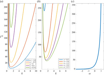
 $k$. Figure 2 shows
 $\varGamma ^2$ as a function of
 $k$ for representative values of
 $\omega$ with
 $\alpha =1$ in (a) and for representative values of
 $\alpha$ with
 $\omega =0.5$ in (b). We see in (a) that the minimum of
 $\varGamma ^2$ over
 $k$ increases as
 $\omega$ increases. In figure 2(c) we show the minimum of
 $\varGamma ^2$ over
 $k$ as
 $\omega$ varies with
 $\alpha =1$. We see that, as was the case for the unbounded problem, the flow stabilises as
 ${\omega }/{\alpha ^{2/3}}\rightarrow 1.154$ from below. That result is also found for other values of
 $\alpha$. Note also that the minimum of
 $\varGamma ^2$ shown in (c) goes to zero like
 $\vert \omega \vert ^{-1}$ when
 $\omega$ becomes large and negative.
Results for the bounded case for propagating waves with  $\beta =0$. Results in (a) are calculated with
 $\alpha =1$ at various values of
 $\omega$ whilst (b) has
 $\omega =0.5$ and various values of
 $\alpha$. (c) Shows the minimum of
 $\varGamma ^2$ over
 $k$ at different values of
 $\omega$ with
 $\alpha =1$.

4.2. Stationary oblique wavy walls
Now let us consider the oblique case for stationary waves, here the neutral curve is defined by (3.13). For the unbounded problem we take  ${\mathcal {H}}_1=1$ and, because of our choice of length scale length scale, we set
 $\alpha ^2+\beta ^2=1$. If we then vary
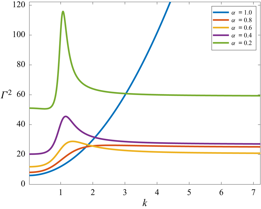
 ${\alpha }/{\beta }$ we will determine how the wall amplitude needed for instability depends on the alignment of the wave crests. Figure 3 shows the neutral value of
 $\varGamma ^2$ as a function of
 $k$ for different values of
 $\alpha$ with
 $\alpha ^2+\beta ^2=1.$ We observe the surprising result that when
 $\beta \ne 0$ the neutral value of
 $\varGamma ^2$ tends to a finite value when
 $k\rightarrow \infty$, that result is confirmed by taking the limit
 $k\rightarrow \infty$ in (3.13) for any
 $\beta \ne 0$.
Results for oblique wall undulations in an unbounded region for  $\alpha ^2+\beta ^2=1$ and different values of
 $\alpha$. Note that
 $\alpha =1$ corresponds to the aligned case.

Figure 3 indicates that, for  $\alpha$ less than approximately 0.2, the instability occurs first as
 $k\rightarrow 0$ and the most unstable configuration is the aligned one. However, around
 $\alpha =0.2$ an oscillation in the curve is seen to develop near
 $k=1$, this is the initial stage of resonance as the spanwise wavenumber of the vortex and the undulation approach each other as
 $\alpha \rightarrow 0.$ The oscillation becomes more pronounced as
 $\alpha \rightarrow 0$ but the neutral curve moves upwards with
 $\varGamma ^2 \sim \alpha ^{-({1}/{3})}$ and so, whilst interesting, it is perhaps not significant since the aligned and indeed less oblique configurations are more unstable. The upshot then is that for the unbounded case the aligned configuration is the most dangerous, but oblique configurations have an infinite band of possible unstable wavenumbers. Thus, for any
 $\beta \ne 0$, as
 $k$ is increased from zero there is a value of
 $k$ beyond which that particular configuration is more unstable than the
 $\beta =0$ configuration. A similar resonance will be found in the transpiration problem where it has a more profound effect on the instability problem.
The bounded problem corresponds to solutions of (3.13) with  ${\mathcal {H}}_1={\mathcal {H}}(k)$ and
 $\alpha, \beta$ no longer constrained such that
 $\alpha ^2+\beta ^2=1.$ Some typical results are shown in figure 4(a). The black and red curves correspond to walls with
 $\alpha ^2+\beta ^2=1,2$, respectively, with the continuous and dashed curves corresponding to aligned and oblique configurations, respectively. For the case
 $\alpha ^2+\beta ^2=1$ we see that the most dangerous configuration corresponds to the oblique mode with
 $k\gg 1$ whilst for
 $\alpha ^2+\beta ^2=2$ the most dangerous configuration is the aligned one.
Results for the bounded problem, i.e. Couette flow, with stationary walls. In (a) the black/red curves correspond to waves with  $\alpha ^2+\beta ^2=1,2$. We see that for
 $\alpha ^2+\beta ^2= 2$ the most dangerous mode is the aligned one, but for
 $\alpha ^2+\beta ^2=1$ it is the oblique mode. (b) Shows
 $\varGamma ^2$ for the
 $\beta =0$ (dashed curve) case and the value of
 $\varGamma ^2_m$ for the most dangerous oblique wall of the same wavelength.

The results shown in figure 4(a) suggest that there is a significant change in the effect of obliqueness when  $[\alpha ^2+\beta ^2]$ decreases. In order to quantify that change we fix
 $\alpha ^2+\beta ^2$, and vary
 ${\beta }/{\alpha }$ to find the most dangerous configuration at any
 $k$, we then vary
 $k$ to find
 $\varGamma _m([ \alpha ^2+\beta ^2]^{1/2})$ the lowest value of
 $\varGamma$ over all values of
 $k, {\beta }/{\alpha }$ for a wall of fixed wavelength. The result of that calculation is shown in figure 4(b). We see that at
 $\sqrt {\alpha ^2+\beta ^2}\simeq 1.0778$ the most dangerous mode switches from an oblique configuration to the aligned one. When the oblique configuration is the most unstable, it corresponds to the large
 $k$ form of the disturbance.
In order to predict the critical value of the wall wavelength where the change in behaviour occurs we first note from (3.13) that for  $k$ large
 ${9Ai'^2(0)\alpha ^{4/3}\beta ^2}\varGamma ^2\simeq {4[\alpha ^2+\beta ^2]^2}$. It follows that, for a wall of fixed wavenumber
 ${\mathcal {A}}=\sqrt {\alpha ^2+\beta ^2}$, the minimum of
 $\varGamma$ occurs at large
 $k$ with
 ${\beta }/{\alpha }=\sqrt {\frac {3}{2}}$ so that for large
 $k$ the most dangerous configuration has
 \begin{equation} \varGamma^2\simeq \frac{2^{4/3}5^{5/3}{\mathcal{A}}^{2/3}}{27Ai'^2(0)}. \end{equation}
On the other hand, noting that the aligned problem has  ${\mathcal {A}}=\alpha$, the neutral configuration in that configuration has
 \begin{equation} \varGamma^2=\frac{2[{\mathcal{A}}^2+k^2]{\mathcal{H}}(k)}{5Ai'^2(0){\mathcal{A}}^{4/3}}. \end{equation}
If we equate the right-hand sides of (4.1) and (4.2) we obtain an equation linking  $k$ and
 ${\mathcal {A}}$. But
 $k$ corresponds to a minimum of the right-hand side of (4.2) so differentiating with respect to
 $k$ we obtain a second equation linking
 $k$ and
 ${\mathcal {A}}$. Eliminating
 ${\mathcal {A}}$ then yields
 \begin{equation} k{\mathcal{H}}'-\frac{ 2^{2/3}27}{5^{8/3}}{\mathcal{H}}^2+2{\mathcal{H}}=0, \end{equation}
and calculations show that there is one root of the above equation with  $k=1.1715$ and then
 ${\mathcal {A}}=1.0778.$ Therefore, when the wall wavelength, scaled on the channel depth, is bigger than
 $5.83$ the oblique configuration with the crests inclined at
 $39.4^{\circ }$ to the flow direction is the most unstable one and
 $\varGamma _m$ goes to zero like the inverse
 $\frac {1}{3}$ power of the wavelength. This surprising result is due to the instability persisting for large
 $k$ in the oblique case. In fact for sufficiently large
 $k$ the vortex shrinks into the viscous wall layer and
 $\varGamma$ then increases with wavenumber, we will comment on that limit in the conclusion.
5. Results for transpiration
5.1. Propagating wall transpiration
If the wave propagates in the same direction as the unperturbed flow then we take  $\beta =0$ and the neutral curve is defined by (3.14) and is independent of
 $\omega$. For the unbounded problem
 $\varLambda ^2=6(\alpha ^2+k^2)$ so that instability occurs first at
 $k=0$.
For the bounded problem we take  ${\mathcal {H}}_1={\mathcal {H}}$ and the neutral curves for a range of values of
 $\alpha$ are as shown in figure 5(a). We see that the minima occur at decreasing values of
 $k$ as
 $\alpha \rightarrow 0.$ The minimum of
 $\varLambda ^2 \simeq 8.85$ and using (2.12) we can define a neutral curve in the
 $R-\delta$ plane for small
 $\delta$. That curve is shown in figure 5(b); also shown are results taken from Floryan (Reference Floryan2002), who considered the problem numerically. We see that there is excellent agreement between the asymptotic and numerical results. Based on the computational results Floryan concluded that for large
 $R$ the transpiration amplitude varied like
 $R^{-1.15}$, the higher power than
 $R$ compared with (2.12) being found because no dependence on
 $\log R$ was anticipated.
Results for the aligned bounded case in the presence of transpiration. (a) Shows  $\varLambda ^2$ as a function of
 $k$ for different values of
 $\alpha$. (b) Compares our asymptotic prediction of the transpiration amplitude/Reynolds number dependence with the numerical results of Floryan (Reference Floryan2002).

5.2. Stationary oblique wall transpiration
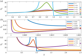
In the case when the transpiration wave crests are not aligned with the flow direction the neutral curve is defined by (3.15). Results for the unbounded case are shown in figure 6(a) where we have plotted  $\varLambda ^2$ as a function of
 $k$ for different values of
 $\alpha$ with
 $\alpha ^2+\beta ^2=1.$ We see that the aligned case is initially the most unstable as
 $\alpha$ decreases from unity but at a critical value of
 $\alpha$ there is a switch to the oblique mode, and that occurs in the limit
 $k\rightarrow \infty$. It is readily shown from (3.15) that this switch happens when
 $\alpha =\sqrt {\frac {1}{3}}$.
(a) Shows  $\varLambda ^2$ as a function of
 $k$ for a range of values of
 $\alpha$ with
 $\alpha ^2+\beta ^2=1$ for the unbounded problem. (b) Is an enlargement of (a) near
 $k=1$ showing small
 $\alpha$ behaviour. (c) Shows the corresponding results for the bounded problem again with
 $\alpha ^2+\beta ^2=1$. Note that in both cases
 $\alpha =1$ corresponds to the case when the undulation wave crests are perpendicular to the flow direction.

Further decreasing  $\alpha$ an oscillation in the neutral curve develops near
 $k=1$ and eventually the minimum of
 $\varGamma$ moves from
 $k=\infty$ to a value close to
 $k=1$. As
 $\alpha$ approaches zero the oscillation has a minimum approaching zero at a value of
 $k$ increasingly close to
 $k=1$. This is the same resonance observed in the wavy wall case and it occurs as the vortex wavenumber approaches the spanwise transpiration wavenumber for
 $\alpha \ll 1$. It can be shown from (3.15) that when
 $\alpha \rightarrow 0$ the neutral curve approaching
 $k=1$ from the right develops a vertical asymptote and splits into branches to the right and left of
 $k=\beta +O(\alpha ^2)$. The small
 $\alpha$ behaviour near
 $k=1$ is enlarged in figure 6(b). We see that location of the minimum of
 $\varLambda$ approaches
 $k=1$ as
 $k$ decreases and it can be shown from (3.15) that
 $\varLambda ^2$ at the minimum is
 $O(\alpha )$ Thus the most dangerous oblique orientation has the wave crests almost parallel to the flow direction with
 $\varLambda ^2\sim \alpha$. The VWI formulation fails if
 $\alpha =0$ and so for small
 $\alpha$ a new structure appears. We do not investigate that new regime but expect that the new structure is similar to the boundary region scenario used by Deguchi, Hall & Walton (Reference Deguchi, Hall and Walton2013) to describe long wave exact coherent structures.
We saw earlier that a similar resonance occurs for wavy walls, but the key difference is the factor  $\alpha ^{-({4}/{3})}$ which appears in (3.12) and (3.13). Apart from that factor (3.12), (3.13) and (3.14), (3.15) have similar asymptotic structures when
 $\beta \sim k, \alpha \ll 1$. But the factor
 $\alpha ^{-({4}/{3})}$ pushes the value of
 $\varGamma ^2$ where resonance occurs to values of
 $\varGamma ^2\sim \alpha ^{-({1}/{3})}$ and so the resonant interaction does not play a dominant role in the oblique wall undulation problem.
The results for the bounded problem are shown in figure 6(c) and, apart from the curves now having left hand branches as  $k\rightarrow 0$, the results are very similar to the unbounded case with a resonant interaction developing at
 $k=\beta =1$ when
 $\alpha \rightarrow 0$.
6. Conclusion
We have given a strongly nonlinear description of instabilities caused by boundary forcing of a rather general form. The description generalises the linear stability theory first given in H1 in connection with instabilities caused by wavy walls. The latter approach, and the much more general one developed here, show conclusively that streamwise vortex instabilities induced by forcing do not require regions of reversed flow. We applied the more general approach to two particular problems, wavy wall and transpiration induced instabilities in finite and semi-infinite regions. In each case we considered forcing in the form of a wave either propagating in the unperturbed flow direction or a stationary oblique wave.
Surprisingly it was found that in the transpiration problem allowing the wave to propagate in the flow direction has no effect on the stability problem. For the wavy wall we found that a wave propagating upstream leads to the flow becoming progressively destabilised as the magnitude of the wave speed increases. On the other hand downstream propagation leads to the flow being stabilised with the wave amplitude needed for instability increasing monotonically with the wave speed and tending to infinity as a critical wave speed is reached. That result has implications for devices used to promote mixing by inducing instabilities by boundary forcing.
For the case of oblique waves significant new effects come into play. For both the wavy wall and transpiration problems any obliqueness causes the flow to remain unstable as the spanwise wavenumber tends to infinity. Moreover, given a fixed forcing wavelength, it is possible for the oblique configuration to be the most unstable one when disturbances of all spanwise wavenumbers are considered. In particular, for the bounded wavy wall problem, there exists a critical wavelength above which the most unstable mode switches to the oblique case. For the transpiration problem in both the bounded and unbounded cases a resonance occurs when the vortex wavelength coincides with the forcing spanwise wavelength as the streamwise wavenumber becomes small. Thus, as the forcing wave crests become almost parallel to the unperturbed flow direction, the wall amplitude needed for instability becomes arbitrarily small and the VWI structure will eventually fail. We have not investigated that limit here but expect it is similar to that discussed for a closely related problem in exact coherent structures by Deguchi et al. (Reference Deguchi, Hall and Walton2013).
Now let us make some remarks concerning the universal nature of our results, we concentrate on the wall undulation problem but comment briefly on the transpiration problem. For the unbounded problem we used the forcing wavelength as a typical length scale and it was assumed small compared with the length scale of the unperturbed flow. More precisely we used  ${b}/{2{\rm \pi} }$ where
 $b$ is the dimensional wall wavelength as the length scale and if
 $h$ is the dimensional amplitude of the undulations it follows that
 $\epsilon ={{\rm \pi} h}/{b}$. Our formulation of the unbounded problem corresponds to an infinitely deep shear flow interacting with boundary forcing operating on a short length scale so the nature of the unperturbed flow only influences the structure found through the friction velocity. Note also that the Reynolds number
 $R$ used in the formulation of the unbounded problem satisfies
 $R={R_f^2}/{4{\rm \pi} ^2}$ where
 $R_f$ is the friction Reynolds number.
Suppose then that we consider (3.12) and note that the most unstable configuration has  $k=0$ and take
 $\alpha =1, {\mathcal {H}}_1=1.$ Using (2.11) it follows that instability occurs when
 \begin{equation} \frac{h}{b}>\frac{2^{5/6}{\rm \pi}^{1/3}\varGamma_c(\omega)}{ R_f^{4/3}\sqrt{\log{R_f}}}. \end{equation}
Here,  $\varGamma _c(\omega )$ is given by (3.12) with
 $\alpha =1,\ k=0,\ {\mathcal {H}}_1=1$ and, in view of our dimensionalisation, the frequency
 $\omega$ used in the definition of
 $\xi _1$ is given in terms of the dimensional frequency
 $f$ by
 $\omega ={f \nu }/{u_s^2}$. The criterion (6.1) is a universal result which applies to all shear flows over a wavy wall of small amplitude and wavelength small compared with the length scale of the unperturbed flow. The criterion depends on the particular shear flow only through the friction velocity
 $u_s$ used to define
 $R_f$ and
 $\omega$. Note further that
 $\varGamma _c \rightarrow \infty$ as
 $\omega \rightarrow 1.154$ from below and goes to zero like
 $\vert \omega \vert ^{-1}$ for rapidly upstream propagating waves. A universal result similar to (6.1), independent of
 $\omega$, can be written down for transpiration waves. For the bounded problems with either an aligned propagating wavy wall or transpiration forcing the neutral configuration depends on the basic state and so no universal results can be written down.
Now consider stationary oblique wall undulations and see what universal results can be inferred in that case. For the unbounded problem figure 3 shows the neutral values of  $\varGamma$ as defined by (3.13) with
 $\alpha ^2+\beta ^2=1, {\mathcal {H}}_1=1$ as a function of
 $k$ for various values of
 $\alpha.$ If we define
 $\varGamma _d$ to be the minimum of
 $\varGamma$ over
 $k$ for a given
 $\beta /\alpha$ then (3.13) predicts that instability occurs when
 \begin{equation} \frac{h}{b}>\frac{2^{5/6}{\rm \pi}^{1/3}\varGamma_d \left(\dfrac{\beta}{\alpha}\right)}{ R_f^{4/3}\sqrt{\log{R_f}}}, \end{equation}
and (6.1) and (6.2) coincide when  $\omega =0$ in the propagating case and
 $\beta =0$ in the oblique case. Note also that
 $\varGamma _d$ corresponds to
 $k=0$ for
 $\alpha _c<\alpha <1$ where
 $\alpha _c\simeq 0.2$ but further decreasing
 $\alpha$ the most dangerous mode moves to a finite value of
 $k$. Once again the instability criterion (6.2) is a universal one for a given wall orientation.
For the bounded problem the wavelength of the forcing is comparable to the length scale of the unperturbed flow so at first sight we expect no universality in our results. Figure 4(b) shows the variation of  $\varGamma _m$, the minimum of
 $\varGamma$ over
 $k, {\beta }/{\alpha }$, with
 ${\mathcal {A}}=\sqrt {\alpha ^2+\beta ^2}$. For waves with
 ${\mathcal {A}}>1.0778$ the aligned configuration is the most dangerous one and the criterion for instability cannot be applied to other flows since it depends on the bounded flow being Couette flow. Note here that for a more general basic bounded flow
 $(\bar {u}(y),0,0)$ we simply solve for the vortex flow
 $(u_1,v_1,w_1)$ in
 $0< y<1$ with the Couette flow profile
 $\bar {u}=y$ replaced by
 $\bar {u}$, that leads to a modified form of (3.6). However, when
 ${\mathcal {A}}<1.0778$ the most unstable configuration follows a path into the origin, and along that path the corresponding vortex mode has
 $k\rightarrow \infty.$ We now show how the surprising result that
 $\varGamma _m \rightarrow 0$ as
 ${\mathcal {A}}\rightarrow 0$ is actually a manifestation of universality.
We first note that the Reynolds number  $R$ for the Couette flow problem is related to the friction Reynolds number
 $R_f$ by
 $R_f^2=R({b^2}/{4{\rm \pi} ^2d^2})$ and
 ${\mathcal {A}}$ in (4.1) is given by
 ${\mathcal {A}}= {2{\rm \pi} d}/{b}$ and
 $h=2\epsilon d$. Using (2.11) the condition (4.1) which determines the most unstable configuration for
 ${\mathcal {A}}<1.0778$ can be written in terms of the friction Reynolds number as
 \begin{equation} \frac{h}{b}>\frac{2^{3/2}5^{5/6}{\rm \pi}^{1/3}}{3^{3/2}\vert Ai_0'\vert R_f^{4/3}\sqrt{\log R_f+\log\left({\dfrac{d}{b}}\right)}}. \end{equation}
The above result defines the criterion for instability for walls with  ${\mathcal {A}}<1.0778$, or equivalently walls with
 ${b}/{d}>5.83.$ Without the second term inside the square root sign (6.3) is a universal result. Formally the result is valid for
 $R_f\gg 1$ with
 ${d}/{b}=O(1)$ so that the second term in the square root is small compared with the first one and so in practice the dependence on the presence of the upper wall is weak. Thus the effect of the vortex wavenumber being large and confining the vortex to the vicinity of the lower wall overrides the finite depth effect. Moreover, what was at first sight a surprising result in (4.1) that
 $\varGamma _m^2$ goes to zero when
 ${\mathcal {A}}\rightarrow 0$ is simply a manifestation of the instability criteria now being more appropriately expressed in terms of flow properties near the wall where the vortex is concentrated.
Finally we explain briefly the fate of the oblique modes which persist to arbitrarily large values of the vortex wavenumber. We first note that for large  $k$ the streamwise vortex structure approaches the wall and is confined to a layer of depth
 $k^{-1}$. When that thickness coincides with the viscous wall layer the VWI structure collapses and the wave and vortex fields couple. Since there is no longer a logarithmic growth associated with the spanwise roll velocity, it can be shown that we now need to take
 \begin{equation} \epsilon=\frac{\hat{\varGamma}}{R^{2/3}}, \end{equation}
in order to close the interaction for the wavy wall problem. The instability problem is then fixed in terms of an eigenvalue problem associated with partial differential system which determines  $\hat {\varGamma }$ in terms of the scaled wavenumber
 $\hat {k}={k}/{R^{1/3}}$. In this regime the vortex and wave are coupled and cannot be solved for independently. On taking the limit of
 $\hat {k}$ tending to zero the double layer structure found previously returns and it can be shown that, if
 $\varGamma _F(\beta, \alpha )$ is the large
 $k$ limit of
 $\varGamma$ for a given wall with
 $\beta \ne 0$, then for small
 $\hat {k}$ we find that
 \begin{equation} \hat{\varGamma}\simeq\frac {3^{1/2} \varGamma_F} {\sqrt {\vert \log{ \hat{k}}\vert}}+\cdots, \end{equation}
and this connects the solution with the large  $k$ limit of the
 $k=O(1)$ solution. It follows that moving away from the
 $k=O(1)$ regime towards the
 $k=O(R^{1/3})$ regime
 $\epsilon$ takes the form
 \begin{equation} \epsilon=\frac{\varGamma_F} {R^{2/3} \sqrt{\log R-3\log{k}}}. \end{equation}
The factor  $3$ multiplying the
 $\log k$ term means that in practice viscous effects will cause
 $\epsilon$ to increase at relatively low values of
 $k$. A similar result applies to the transpiration case.
Acknowledgements
The author thanks the referees for their constructive comments on this paper.
Declaration of interests
The author reports no conflict of interest.