Introduction
Bulk-metallic glasses (BMGs), as promising materials with unique structural features and outstanding mechanical, physical, and chemical properties, have been extensively studied for potential applications in various fields since they were first discovered in 1960 by Duwez and co-workers.[Reference Wang1] However, the relationship between the mechanical properties and chemical composition of BMGs remains unclear due to the poor understanding of the underlying physics. No successful analytic model is currently available to design a new BMG with targeted properties. As a result, the discovery and optimization of potential materials for application relies on the time-consuming traditional paradigms of materials science and engineering.[Reference Ramprasad, Batra, Pilania, Mannodi-Kanakkithodi and Kim2]
Along with the fast development of artificial intelligence, the paradigm of machine learning (ML) and materials informatics, which unifies the knowledge learned from experiments, theory, computations, and simulations, is rapidly becoming popular in materials science.[Reference Ramprasad, Batra, Pilania, Mannodi-Kanakkithodi and Kim2–Reference Ren, Ward, Williams, Laws, Wolverton, Hattrick-Simpers and Mehta7] Integrating artificial intelligence with materials science and engineering will accelerate the design and discovery of advanced materials. Several research groups have used ML to study metallic glasses. For example, Sun and co-workers used support vector machine to study the glass-forming ability (GFA) of binary metallic alloys with random compositions.[Reference Sun, Bai, Li and Wang5] Ward and Ren applied an ML approach to metallic glasses containing three or more elements.[Reference Ward, O'Keeffe, Stevick, Jelbert, Aykol and Wolverton6,Reference Ren, Ward, Williams, Laws, Wolverton, Hattrick-Simpers and Mehta7] The findings of these studies suggest that ML has great potential to aid in discovery of new metallic glasses with good GFA.
In this work, we used ML to study BMGs with the aim to predict their elastic moduli (bulk modulus K and shear modulus G) and GFA. A four-step procedure was followed: (1) data collection: two sets of experimental data on metal–metal BMGs were collected from the literature, one set containing the elastic moduli of 219 BMGs and the other containing the critical casting diameters of 442 BMGs; (2) feature selection: the best subset selection (BSS) algorithm was applied to select the best features from feature candidates; (3) parameter tuning: the parameters of the ML model were tuned by an optimization technique; and (4) ML model validation: the ML model was trained and tested by leave-one-out cross-validation (LOOCV) (Fig. 1).
Four-step procedure used in this study: (1) data collection; (2) feature selection; (3) parameter tuning; and (4) ML validation.

Data collection and treatment
Data collection
Two datasets were used in this work: (1) an elastic modulus dataset and (2) a critical casting diameter dataset. In the elastic modulus dataset (shown in Table S1 in Supplementary Material), the shear modulus and bulk modulus of 219 metal–metal BMGs were collected.[Reference Wang1,Reference Liu and Zhang8] The 219 alloys included four Ca-based, 23 Cu-based, four Hf-based, 69 LT-based (LT = Ce, Dy, Er, Gd, Ho, La, Lu, Nd, Pr, Sm, Tb, Tm, and Yb), 21 Mg-based, eight Ni-based, one Sc-based, five Sr-based, four Ti-based, 78 Zr-based, and two high-entropy alloys. All compositions herein are expressed in atomic fractions. The elastic moduli were measured via the ultrasonic-wave-propagation (UWP) method. For multiple reported values of an elastic modulus of a certain BMG composition, we took the average value as the BMG elastic modulus.
The critical casting diameter dataset (shown as Table S2 in Supplementary Material) contained the characteristic temperatures (glass transition temperature, T g; onset crystallization temperature, T x; and liquidus temperature, T l) and critical casting diameters (D max) for 442 metal–metal BMGs.[Reference Ward, O'Keeffe, Stevick, Jelbert, Aykol and Wolverton6,Reference Ren, Ward, Williams, Laws, Wolverton, Hattrick-Simpers and Mehta7,Reference Long, Liu, Zhong, Yun, Zhao, Liao and Chen9] The 442 alloys included 19 Ag-based, 57 Ca-based, 84 Cu-based, three Hf-based, 111 LT-based, 60 Mg-based, 13 Ni-based, one Sc-based, 20 Ti-based, four Y-based, and 70 Zr-based alloys. All compositions herein are expressed in atomic fractions. Because D max can be affected by the fabrication method, only values of alloys obtained by the copper-mold casting method were chosen. Most of the characteristic temperatures were measured by differential thermal analysis and differential scanning calorimetry at a heating rate of 20 K/min.
Data standardization
The feature standardization method was used to standardize the features, given by
 $${x}^{\prime} = \displaystyle{{x-\bar{x}} \over {\sigma _x}}$$
where  $\bar{x}$ is the average feature value and σ x is the standard deviation.
Support vector regression (SVR) model
WEKA software was used to build an SVR model. A kernel function is often equipped in SVR to convert the feature space into a higher dimensional space. With this function, the output y from any set of features x has a linear correlation in the higher dimensional space, i.e.,
 $$f\,(x) = \langle{w,K\,(x)} \rangle + b,$$
in which K(x) is the kernel function. The parameters w and b are determined by
 $${\rm argmin}\left( {\displaystyle{1 \over 2} \vert \vert w^2 \vert \vert + C\mathop \sum \limits_{i = 1}^m L\,(\,f\,(x_i,y_i))} \right),$$
where C is the penalization parameter and L is the loss function:
 $$L\,(\,f\,(x_i,y_i)) = {\rm max}\lcub {\vert {\,f\,(x_i)-y_i} \vert } \rcub .$$
The used two kernel functions in this research are the radial-basis function (RBF) kernel and the Pearson VII universal kernel (PUK):
RBF: K (x i, x j) = exp ( − γ||x i − x j||2),
PUK:  $K\,(x_i,\; x_j) = \left[ {1 + {\left( {\left( {\sqrt {\Vert x_i-x_j \Vert}^2} \sqrt {2^{1/\omega} -1}} \right)/\sigma} \right)}^2} \right]^{-\omega}. $ The grid search technique was employed to tune RBF parameter γ, PUK parameters ω and σ, and parameter C.
Gaussian process (GP) model
Matlab 2018 software was used to build the GP model. A GP model is characterized such that the output y from any set of features x has a multivariate normal distribution:
 $$y = f\,(x)^TW + \varepsilon, $$
where W is a constant vector, f(x) and ε are Gaussian distributions. The probability densities (PDs) of these two distributions are:
 $$\varepsilon \sim{{\cal N}}\;(0,\sigma ),\quad {\rm PD}\,{\rm (}\varepsilon {\rm )} = \displaystyle{1 \over {\sigma _n\sqrt {2{\rm \pi}}}} \exp \left( {-\displaystyle{{x^2} \over {2\sigma_n^2}}} \right),$$
 $$f(x) \sim{\rm {\cal N}}\;(0,K_f),\quad {\rm PD}\,{\rm (}f{\rm (}x{\rm ))} = \displaystyle{1 \over {K_f\sqrt {2{\rm \pi}}}} \exp \left( {-\displaystyle{{x^2} \over {2K_f^2}}} \right),$$
in which K f is the covariance function, and the following exponential function (EF) was used in this research
 $$K_f = \sigma _f^2 \exp \left( {-\displaystyle{{ \vert \vert x_i-x_j \vert \vert} \over {\sigma_l}}} \right).$$
The σ n, σ f, and σ l were estimated via Matlab automatically.
Results and discussion
Elastic modulus model
Selection of best-performance features
The bulk modulus is fundamentally related to the atomic bonding energy, which is influenced by electronegativity (EN). The bulk modulus depends on the average atomic volume (V A),[Reference Wang, Wang, Yu and Bai10] and the atomic size difference (δ) affects the ratio of K to G in metallic glasses.[Reference Zhao, Bai, Zhang and Liu11] There exists a correlation among the critical cooling rate, elastic modulus, and mixing entropy (S m).[Reference Xia, Meng, Zhang, Ma and Li12] Thus, the feature candidates in the current work include relative electronegativity (REN), total electronegativity (TEN), average atomic volume (V A), atomic size difference (δ), and mixing entropy (S m), which are defined by
 $${\rm REN} = \sum {a_i\lpar {{\rm E}{\rm N}_i-{\rm E}{\rm N}_o} \rpar }, $$
 $${\rm TEN} = \sum {a_i{\rm E}{\rm N}_i}, $$
 $$V_{\rm A} = \sum {a_i\cdot \displaystyle{4 \over 3}\pi r_i^3}, $$
 $$\delta = \sqrt {\sum {a_i{\left( {1-\displaystyle{{r_i} \over {\overline {r_i}}}} \right)}^2}}, $$
 $$S_{\rm m} = -R\mathop \sum \limits_{i = 1}^n a_i\,{\rm ln}\,\phi _i,$$
where a i is the atomic percentage of the i-th constituent, ENo is the Pauling EN of the major element in a BMG, r i is the atomic radius, and  $\overline {r_i} $ is the average value. R is the ideal gas constant and ϕ i is the volume percentage of the i-th component. The replacement of a i by ϕ i in the logarithmic term of S m is due to the effect of the dissimilar size of atoms.[Reference Jiang, Chi and Li13]
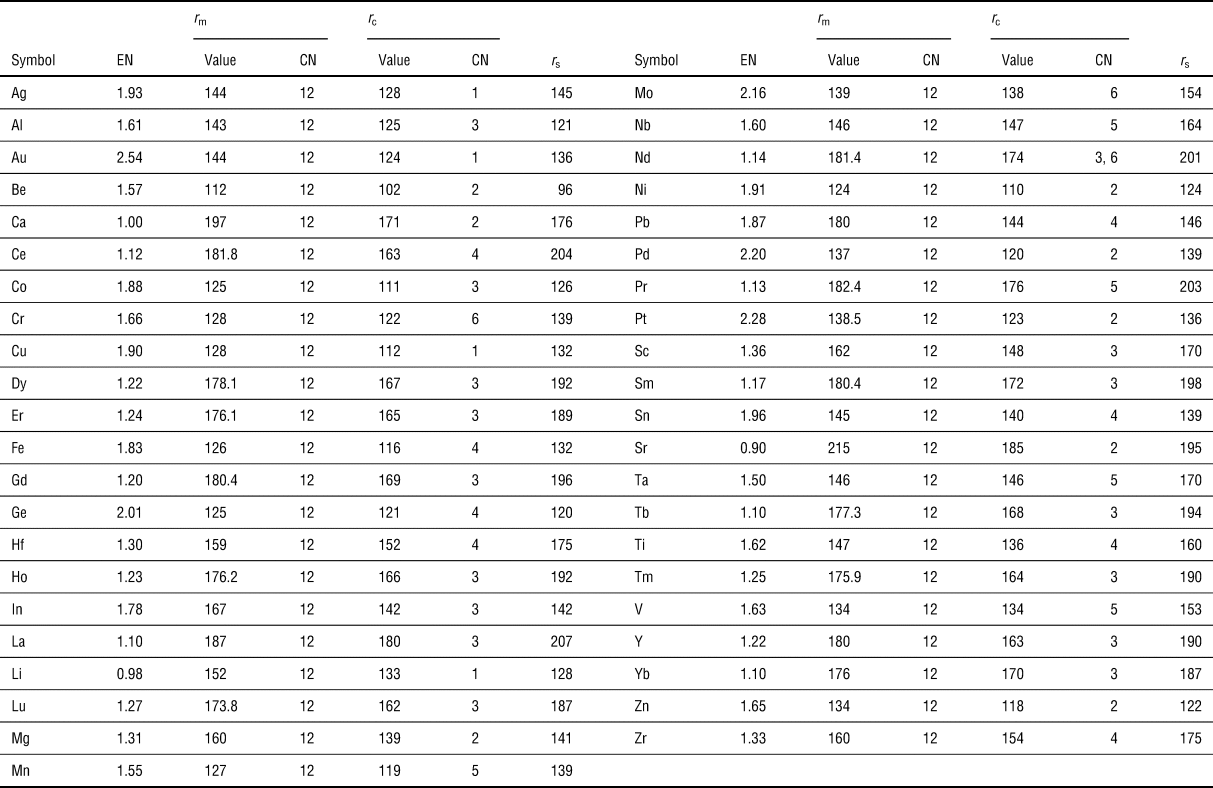
Due to the currently poor understanding of metallic glasses, three types of atomic radii are considered here: the metallic radius (r m), covalent atomic radius (r c), and statistical radius (r s). Their values are shown in Table I and the datasets containing all features, shown in Table II, will be used to train the ML models. The metallic radius,[Reference Inoue and Takeuchi14] which is taken as half of the interatomic distance in the metallic lattice, is widely used as the atomic radius in studies of metallic glasses.[Reference Inoue and Takeuchi14,Reference Laws, Miracle and Ferry15] This radius depends on the nature of the atoms, as well as on the coordination number (CN). The metallic radius of each element in this work is calculated assuming a CN of 12 for a close-packed lattice. Peng et al.[Reference Peng, Li and Huang16] used the covalent atomic radius to study Mg-based metal–metal BMGs, and Lu et al.[Reference Lu, Liu and Dong17] also studied Zr-based metal–metal BMGs using this radius. The covalent radii of Mg and Zr are calculated assuming a CN of 2 and 4, respectively. The CNs[Reference Pyykkö and Atsumi18] used in this work are shown in Table I.
Data of EN[Reference Huheey, Keiter and Keiter19] and atomic radius (pm)[Reference Inoue and Takeuchi14,Reference Pyykkö and Atsumi18,Reference Cordero, Gómez, Platero-Prats, Revés, Echeverría, Cremades, Barragán and Alvarez20] of elements.

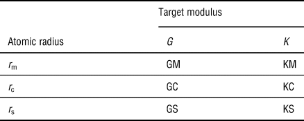
List of original datasets.

The preceding two types of atomic radii assume a constant CN. However, the structures of BMGs are known to be disordered, implying that atoms of the same element might have different CNs.[Reference Miracle21] Thus, the statistical radius,[Reference Cordero, Gómez, Platero-Prats, Revés, Echeverría, Cremades, Barragán and Alvarez20] which is the atomic radius based on a statistical analysis of more than 228,000 experimental bond lengths from the Cambridge Structure Database, was also used in this research.
The BSS method[Reference Guyon and Elisseeff22] was applied to screen these feature candidates. Given m feature candidates, linear least-square regression (LLS) was used to fit for each possible combination of these feature candidates. That is, m LLS models were built that only included one feature candidate, m(m − 1)/2 LLS models were built containing two feature candidates, and so forth.[Reference James, Witten, Tibshirani and Hastie23] The performances of all resulting LLS models were compared to find the best. The root mean square errors (RMSE) was used here as the model fitness, which captures the difference between the actual value (y i) and the LLS-model-predicted value  $(\hat{y}_i)$
 $${\rm RMSE} = \sqrt {\mathop \sum \limits_{i = 1}^n \displaystyle{1 \over n}{\lpar {{\hat{y}}_i-y_i} \rpar }^2}. $$
Two training approaches were adopted here. One approach trains the 219 data in one shot without cross-validation, whose RMSE is usually called the training error and denoted by TrE here. The other approach is the LOOCV method. For the BMG dataset containing 219 samples, the model was trained with 218 data and tested with one data, and cycling 219 times. The 219 testing results were also gaged by RMSE, which is called the testing error and denoted by CVE here. In general, the training error decreases continuously with the model complexity, i.e., with the number and type of features, while there is a minimum in the testing error versus the number and type of features. The minimum in the testing error determines the appropriate features.
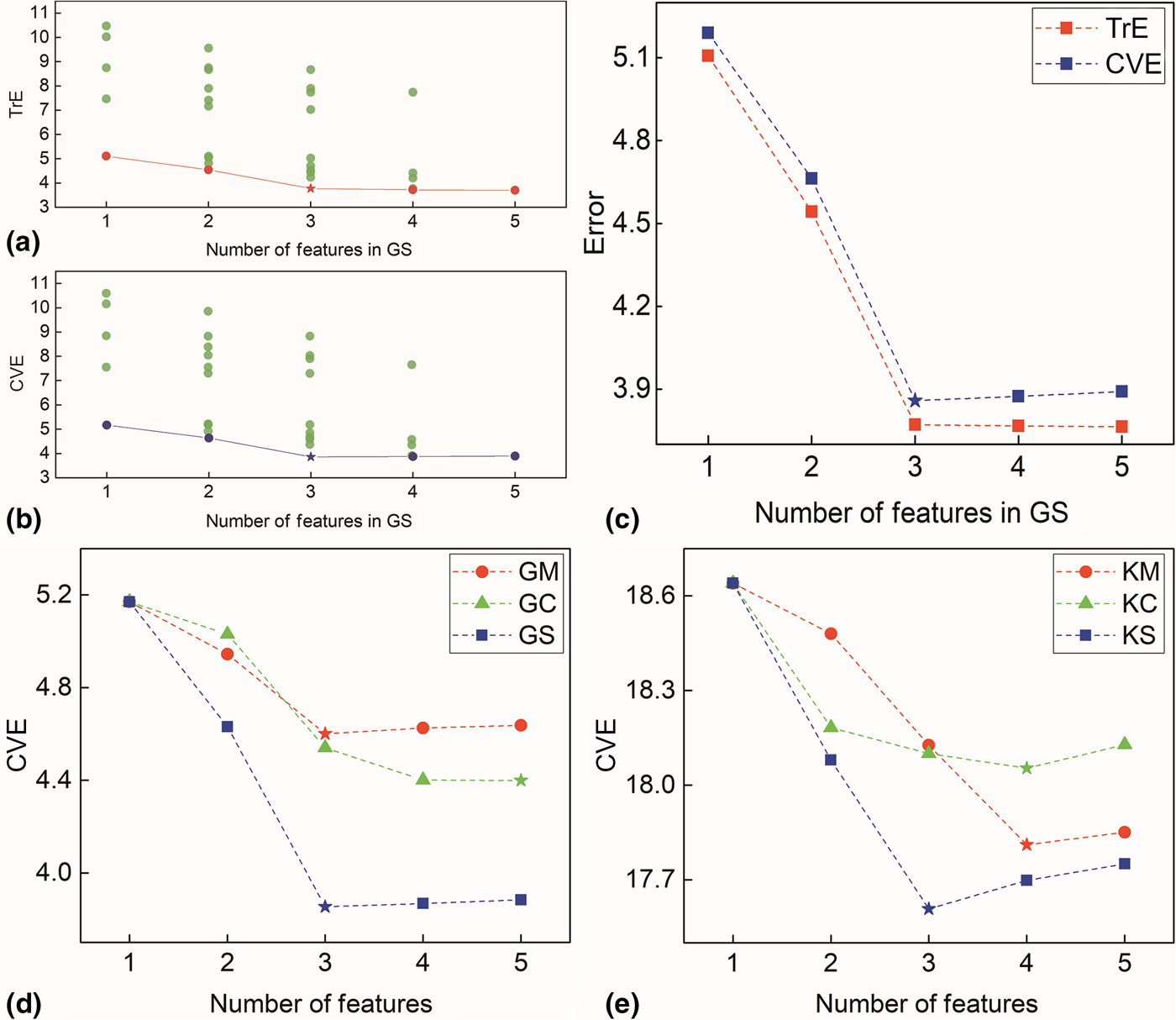
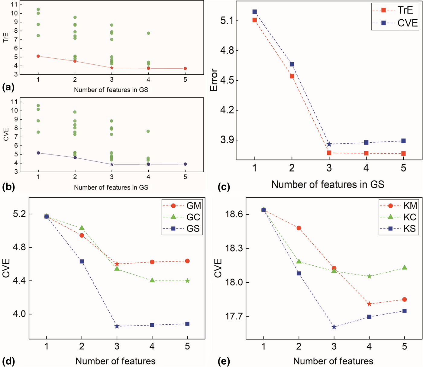
The procedure of applying the BSS method to the example of the GS dataset is shown in Figs. 2(a) and 2(b). Each point stands for an LLS model trained with a different subset of five feature candidates. The TrE and CVE of each model are plotted as a function of the number of features. The TrE shows little improvement beyond three features, while the CVE becomes even worse, as shown in Fig. 2(c). Hence, the best subset for GS contains three features, namely TEN, V A, and δ. This procedure was repeated for the other five datasets, as shown in Fig. 2(d) for G and in Fig. 2(e) for K. The best subset of features for GM is (TEN, V A, and S m); for GC is (REN, TEN, V A, δ, and S m); for GS is (TEN, V A, and δ); for KM and KC is (TEN, V A, δ, and S m); and for KS is (TEN, V A, and δ). These optimal subsets are referred to hereafter as TGs (TGM, TGC, and TGS) and TKs (TKM, TKC, and TKS).
(a) TrE and (b) CVE of each LLS model containing different subsets of GS. The red and blue circles stand for the best LLS model for a given number of features. (c) TrE and CVE value of the best LLS model containing different numbers of features. The CVE of the best LLS model containing a subset of 1–5 features in the training set for (d) G and (e) K.
Selection of the best type of atomic radius by the SVR-RBF model
Grid searches were conducted to obtain the best SVR-RBF model for each training set based on the correlation coefficient (R):
 $$R = \sqrt {\displaystyle{{\mathop \sum \nolimits_{i = 1}^n {\lpar {\widehat{{y_i}}-\bar{y}} \rpar }^2} \over {\mathop \sum \nolimits_{i = 1}^n {\lpar {y_i-\bar{y}} \rpar }^2}}} $$
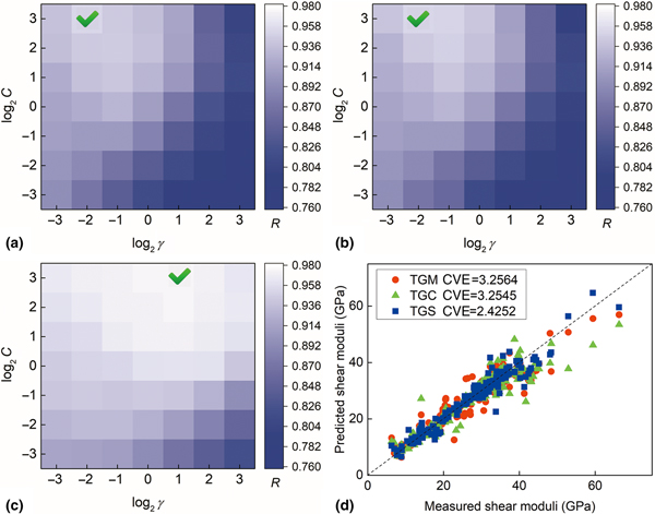
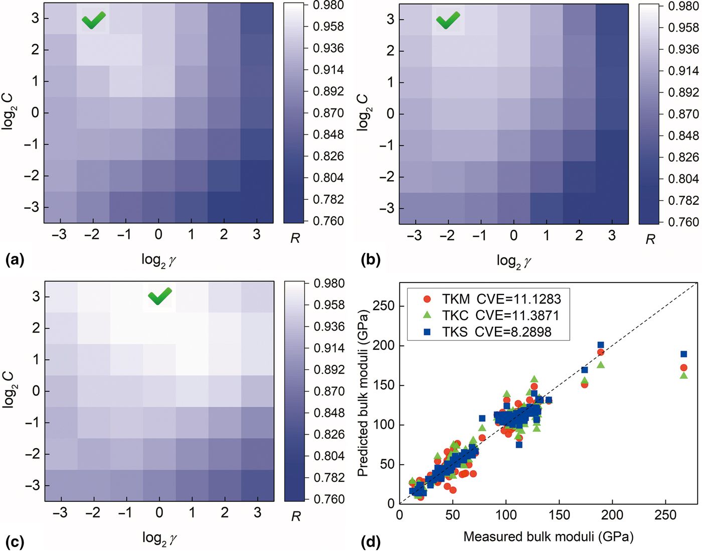
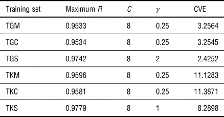
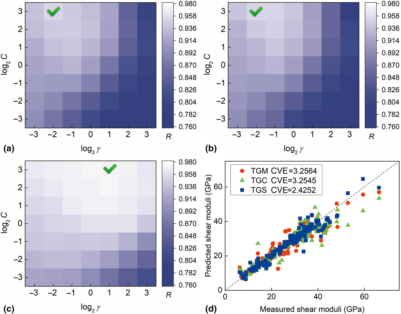
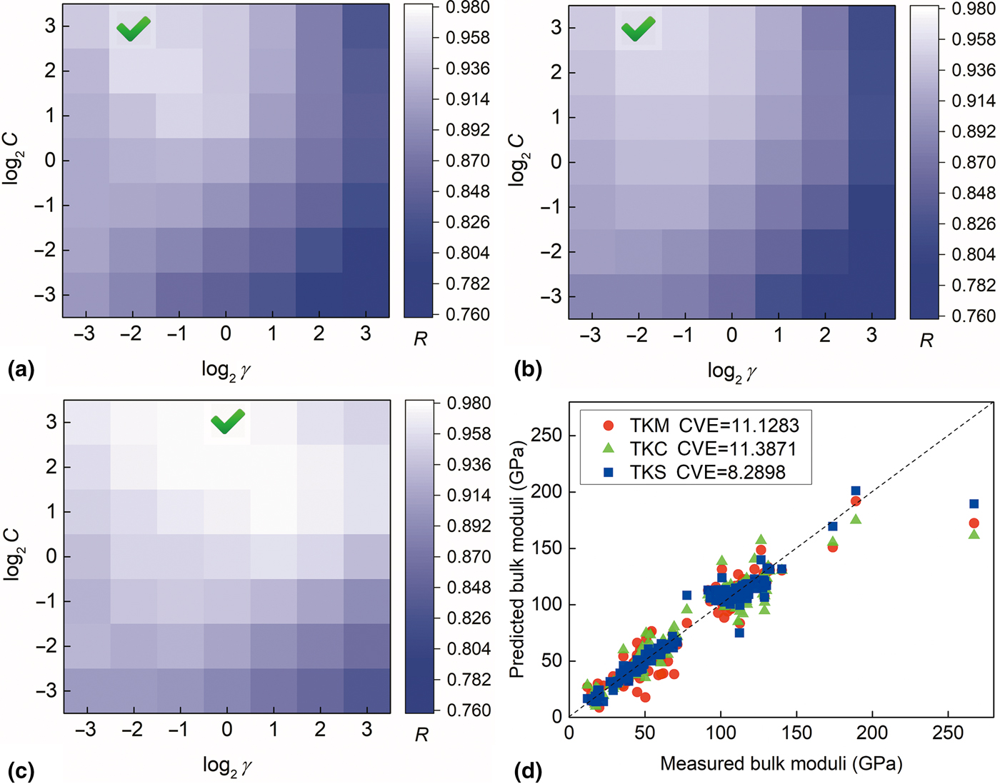
where  $\bar{y}$ is the average of y i, and the R value lies between 0 and 1, with 1 indicating perfect fitting. The R values obtained using different SVR-RBF parameters for the TGs and TKs are shown in Figs. 3(a)–3(c) and 4(a)–4(c), and the maximum values of R are marked with a green check. For comparison, Figs. 3(d) and 4(d) plot the predicted values against the measured values for G and K, respectively, with the best training parameters of the SVR-RBF models. It is clear that the statistical radius performs much better than the metallic and covalent radii. This is therefore the best choice to be used in the ML procedure (Table III).
The performance of the SVR-RBF models on the training datasets for G. R of the SVR-RBF model is found to be maximized at (a) 0.9533 when C = 8, γ = 0.25 for TGM, (b) 0.9534 when C = 8, γ = 0.25 for TGC, (c) 0.9742 when C = 8 and γ = 2 for TGS. (d) Comparison of the predicted G with the measured data.
The performance of the SVR-RBF models on the training datasets for K. R of the SVR-RBF model is found to be maximized at (a) 0.9596 when C = 8 and γ = 0.25 for TKM, (b) 0.9581 when C = 8, γ = 0.25 for TKC, (c) 0.9779 when C = 8, γ = 1 for TKS. (d) Comparison of the predicted K with the measured data.
Result of grid search for SVR-RBF models.

Final ML models for elastic moduli
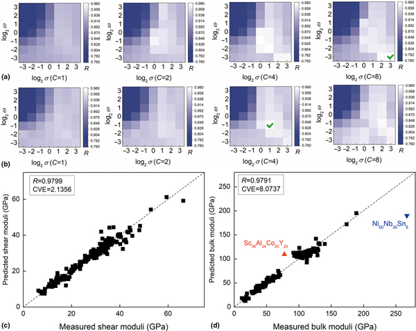
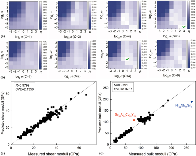
To further generalize the SVR models, PUK[Reference Zhang and Ge24] was applied as a universal kernel function. The PUK function has excellent flexibility due to its adaptable parameters: the penalization parameter (C) and kernel parameters (σ and ω). The R-value of the SVR-PUK-TGS model is maximized at 0.9799 when C = 8, σ = 8, and ω = 0.125 [marked with the green check in Fig. 5(a)], and that for the SVR-PUK-TKS model is maximized at 0.9791 when C = 4, σ = 2, and ω = 0.5 [green check in Fig. 5(b)]. Figures 5(c) and 5(d) show, respectively, the predicted G and K against the measured values, indicating excellent agreement, as evidenced by R > 0.979 for both cases. There are a few exceptions, e.g., the bulk moduli of Sc36Al24Co20Y20 [red triangle in Fig. 5(d)] and Ni60Nb35Sn5 (blue inverted triangle in Fig. 5(d)].
The performance of the SVR-PUK models on the training datasets. R of SVR-PUK model is maximized at (a) 0.9799 when C = 8, σ = 8, ω = 0.125 for TGS, (b) 0.9791 when C = 4, σ = 2, ω = 0.5 for TKS. (c) SVR-PUK-TGS model-predicted moduli G against measured values and (d) SVR-PUK-TKS model-predicted moduli K against measured values.

The alloy Sc36Al24Co20Y20[Reference Xi, Li, Wang, Zhao, Pan and Wang25] is an outlier [see Fig. 5(d)] from the rest of the dataset. This may be because it is the only Sc-based BMG in this dataset. Another outlier is Ni60Nb35Sn5 [see Fig. 5(d)] for which the predicted bulk modulus (189.9 GPa) is much lower than the measured value (267 GPa).[Reference Choi-Yim, Xu and Johnson26] Note that this predicted bulk modulus is close to the experimental value (189 GPa) for an alloy with a similar composition in the dataset, Ni60Sn6(Nb0.8Ta0.2)34. The acoustic properties of Ni60Nb35Sn5 were measured using UWP methods by Haein.[Reference Choi-Yim, Xu, Lind, Löffler and Johnson27] The longitudinal propagation velocity C l was 5.45 km/s and the transverse propagation velocity C t was 2.51 km/s. This allows the elastic modulus of this isotropic material to be calculated using the following equations:
 $$\; x = \left( {\displaystyle{{C_{\rm l}} \over {C_{\rm t}}}} \right)^2,$$
 $$\nu = \displaystyle{{2-x} \over {2-2x}},$$
 $$G = \rho C_{\rm t}^2, $$
 $$K = \displaystyle{{2G\lpar {1 + \nu} \rpar } \over {3\lpar {1-2\nu} \rpar }},$$
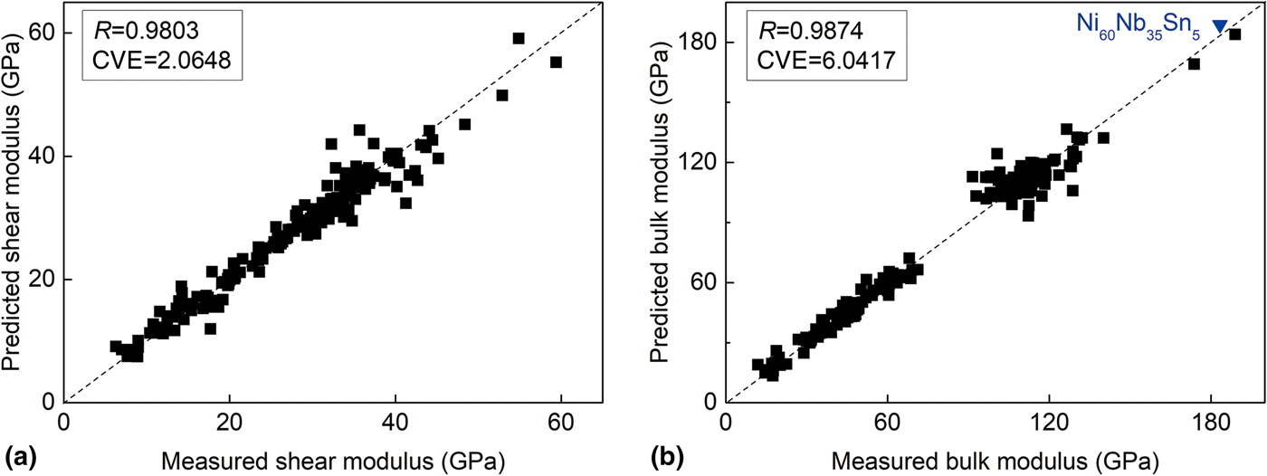
where ν is Poisson's ratio and ρ is the density (8.64 g/cm3 for Ni60Nb35Sn5). The resulting bulk modulus based on Haein's acoustic measurements is 183.3 GPa, which is very close to our prediction of 189.9 GPa. Therefore, we conclude that the measured value (267 GPa)[Reference Choi-Yim, Xu and Johnson26] may not be correct. After updating the elastic modulus for Ni60Nb35Sn5 and removing the data point for the Sc-based alloy, we retrained the ML models, and the resulting predictions are shown in Fig. 6. The predicted bulk modulus of 188.7 GPa for Ni60Nb35Sn5 is very similar to the updated value of 183.3 GPa. The final ML models performed much better, as evidenced by the improved R (>0.980) value.
Predicted moduli against updated measured moduli. (a) SVR-PUK-TGS model-predicted G and (b) SVR-PUK-TKS model-predicted K.

Critical casting diameter model
In the development of new BMGs, another important goal issue is a relatively universal model to assess the GFA. The most reliable and quantifiable GFA indicator of an alloy is the critical cooling rate (R c). However, it is very difficult to measure R c experimentally. A slightly less direct parameter, the critical casting thickness/diameter (D max), was considered in this research. In general, the larger the D max, the higher the GFA. The characteristic temperatures (CTs), T g, T x, and T l, play important roles in the prediction of GFA. Various GFA criteria have been proposed based on the functional relationships among CTs in recent decades.[Reference Long, Liu, Zhong, Yun, Zhao, Liao and Chen9] Twenty GFA criteria, which represent different mathematical combinations of CTs, were evaluated in this research (shown in Table S3 in Supplementary Material). Matlab 2018 software was used to analyze the correlations between the chosen criteria and D max.
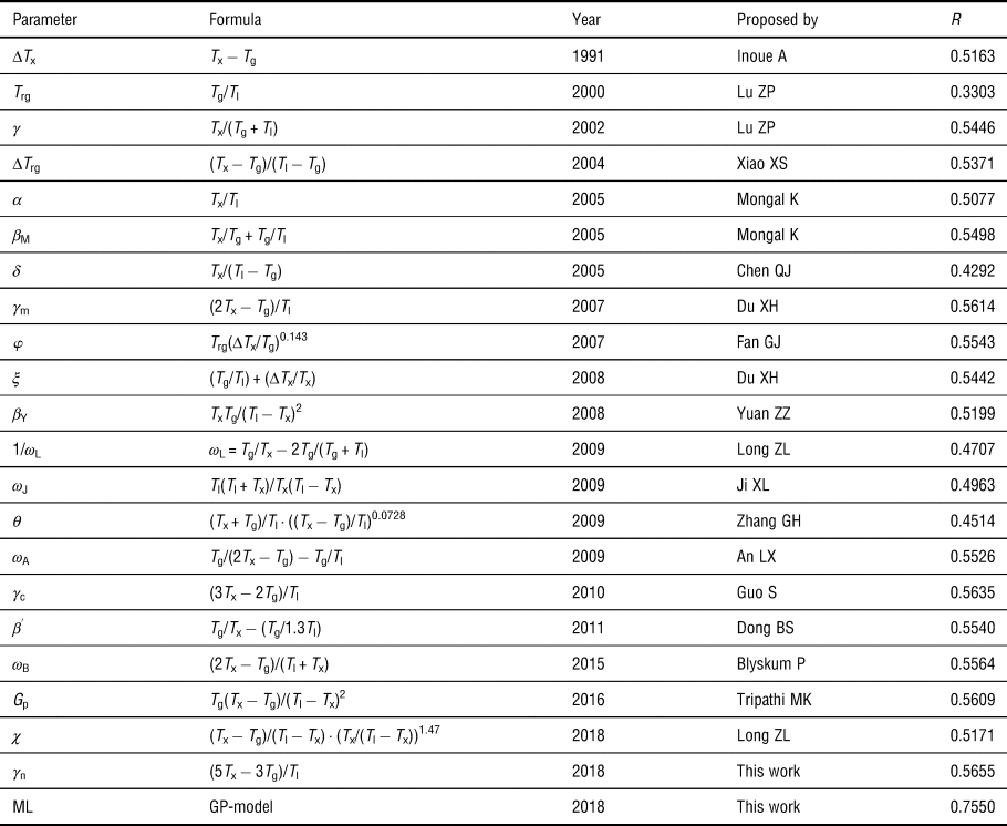
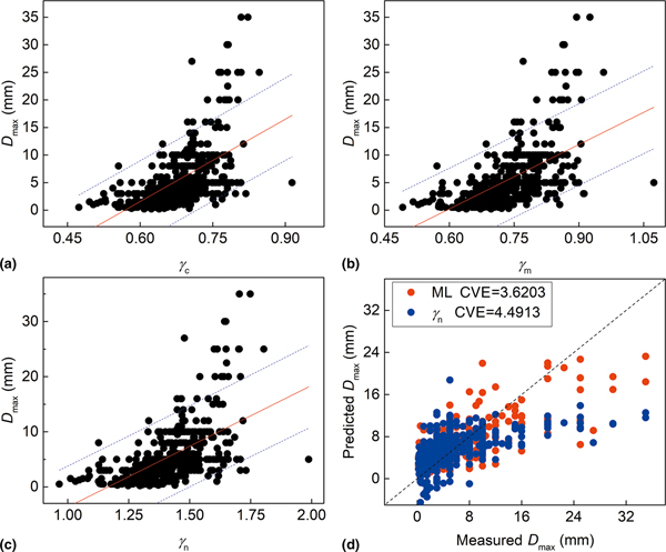
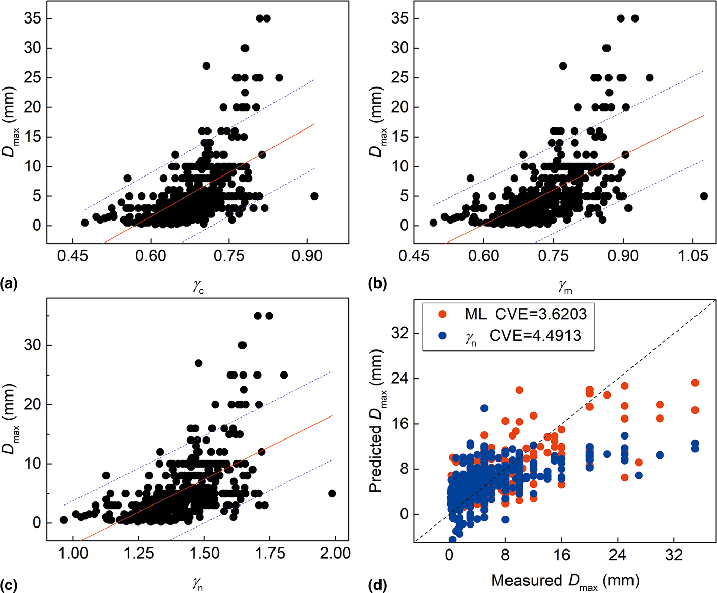
The results in Table IV show the D max-criteria correlations. The highest R value is 0.5635 for the γ c criterion, followed by 0.5614 for the γ m criterion. These two criteria were developed based on T x/T l and (T x − T g)/T l. Thus, we proposed a new parameter γ n (γ n = (AT x − BT g)/T l) for the D max dataset. Setting A and B as 5 and 3 was found to yield the maximum R value (0.5655), which is the highest among all of the tested criteria. The fitting of the best two original GFA criteria and the new γ n criterion is shown in Fig. 7. Then, ML models were built for the prediction of D max using CTs. The ML model based on the GP algorithm with the EF kernel showed the best performance (R = 0.7550), much better than those of the previously developed criteria in the literature. The parameters of the GP model were estimated by Matlab 2018 as σ n = 4.6, σ f = 5.4, and σ l = 0.4. The performance of the GP model is shown in Fig. 7(d). The model shows a similar performance to that of the γ n criterion for small-D max BMGs, but performs much better than that criterion on larger-D max BMGs.
The GFA criteria used in this research, their mathematical formulas, year of proposal, and name of original author.[Reference Long, Liu, Zhong, Yun, Zhao, Liao and Chen9]

Also shown are the values of R for the linear correlation between the predictions using these criteria and the experimental data for D max.
D max versus (a) γ c, (b) γ m, and (c) γ n criteria in 442 metal–metal BMGs. (d) Comparison of the predicted D max by ML model (red circles) and γ n criterion (blue circles) with the measured data.
Conclusions
ML was used to predict the elastic moduli and GFA of metal–metal BMGs. For predicting the elastic moduli, the performance of the ML models was found to be best when using the statistical radius as the definition of atomic radius. The best subset of training features comprised TEN, atomic volume, and atomic size difference. The best ML algorithm was SVR with the PUK function and C = 8, σ = 8, ω = 0.125 for G, and C = 4, σ = 2, ω = 0.5 for K. For predicting the GFA of BMGs via the parameter D max, the ML model GP with an EF performed the best, with σ n = 4.6, σ f = 5.4, and σ l = 0.4.
The ML models showed good performance for the elastic moduli, with small CVE values (2.0648 for G and 6.0417 for K). For predicting GFA, the CVE values of the ML models (3.6203) were also smaller than those using the traditional criteria (4.4913). We believe that the ML models developed in this work can be used to accurately predict the unseen data of metal–metal BMGs, as long as those BMGs contain the metal elements included in our datasets. This work indicates great potential of ML in the design of advanced materials with target properties.
Supplementary material
The supplementary material for this article can be found at https://doi.org/10.1557/mrc.2019.44
Acknowledgments
The work is supported by the National Key R&D Program of China (No. 2018YFB0704404), the Hong Kong Polytechnic University (internal grant nos. 1-ZE8R and G-YBDH), and the 111 Project of the State Administration of Foreign Experts Affairs and the Ministry of Education, China (grant no. D16002).